The $r$-Process in Supersonic Neutrino-Driven Winds: The Roll of Wind Termination Shock

Abstract

Recent hydrodynamic studies of core-collapse supernovae imply that the neutrino-heated ejecta from a nascent neutron star develops to supersonic outflows. These supersonic winds are influenced by the reverse shock from the preceding supernova ejecta, forming the wind termination shock. We investigate the effects of the termination shock in neutrino-driven winds and its roll on the $r$-process. Supersonic outflows are calculated with a semi-analytic neutrino-driven wind model. Subsequent termination-shocked, subsonic outflows are obtained by applying the Rankine-Hugoniot relations. We find a couple of effects that can be relevant for the $r$-process. First is the sudden slowdown of the temperature decrease by the wind termination. Second is the entropy jump by termination-shock heating, up to several $100\,N_{\mathrm{A}}k$. Nucleosynthesis calculations in the obtained winds are performed to examine these effects on the $r$-process. We find that 1) the slowdown of the temperature decrease plays a decisive roll to determine the $r$-process abundance curves. This is due to the strong dependences of the nucleosynthetic path on the temperature during the $r$-process freezeout phase. Our results suggest that only the termination-shocked winds with relatively small shock radii ($\sim 500$ km) are relevant for the bulk of the solar $r$-process abundances ($A\approx 100-180$). The heaviest part in the solar $r$-process curve ($A\approx 180-200$), however, can be reproduced both in shocked and unshocked winds. These results may help to constrain the mass range of supernova progenitors relevant for the $r$-process. We find, on the other hand, 2) negligible roles of the entropy jump on the $r$-process. This is a consequence that the sizable entropy increase takes place only at a large shock radius ($\gtrsim 10,000$ km) where the $r$-process has already ceased.

1. Introduction

Whether the rapid-neutron capture ($r$-process) can take place under the circumstance of core-collapse supernovae has been an unresolved problem for a long time (see Cowan & Thielemann, 2004; Wanajo & Ishimaru, 2006; Arnould et al., 2007, for a recent review). The requisite physical conditions include neutron-rich environment, high entropy, and short expansion timescale to obtain the high enough neutron-to-seed abundance ratio ($\sim 100$) for the production of heavy $r$-process nuclei. The neutrino-heated supernova ejecta (neutrino-driven winds) from a proto-neutron star has been expected as a suitable astrophysical site to fulfil such physical conditions (in particular high entropy and short expansion timescale, Woosley & Hoffman, 1992; Meyer et al., 1992; Woosley et al., 1994; Takahashi et al., 1994; Qian & Woosley, 1996; Cardall & Fuller, 1997; Otsuki et al., 2000; Sumiyoshi et al., 2000; Wanajo et al., 2001; Thompson et al., 2001).

Previous studies confirmed, however, that the spherically expanding winds from a typical proto-neutron star (e.g., $1.4\,M_{\odot}$ with a 10 km radius) cannot attain the requisite physical conditions for the $r$-process. Some mechanisms to cure this problem have been proposed, e.g., general relativistic effects (Cardall & Fuller, 1997; Otsuki et al., 2000; Wanajo et al., 2001; Thompson et al., 2001), magnetic field (Thompson, 2003; Suzuki & Nagataki, 2005), anisotropic neutrino radiation (Wanajo, 2006b), and acoustic heating (Burrows et al., 2007), however, no consensus has been achieved. Recently, Arcones et al. (2007) have suggested that the reverse shock propagating from the preceding supernova ejecta might have important effects on the $r$-process nucleosynthesis. Two-dimensional hydrodynamic studies of core-collapse supernovae have shown that the outflow driven by neutrino heating develops to be supersonic, which eventually decelerate by the reverse shock from the outer layers (e.g., Janka & Müller, 1995, 1996; Burrows et al., 1995; Buras et al., 2006). Arcones et al. (2007) have explored the effects of the reverse shock on the properties of neutrino-driven winds by one-dimensional, long-time hydrodynamic simulations of core-collapse supernovae. They have found that, in their all models ($10-25\,M_{\odot}$ progenitors), the outflows become supersonic and form the “termination shock” when colliding with the slower preceding supernova ejecta. This condition continues until the end of their computations (10 seconds after core bounce) in their all “standard” models (with reasonable parameter choices). Their results show that the entropy abruptly increases and the temperature continues to decrease very slowly in the termination-shocked winds. Arcones et al. (2007) have suggested that the strongly time-dependent behaviours of the shocked conditions would play a non-negligible role to the $r$-process nucleosynthesis.

Systematic nucleosynthesis calculations with the termination-shocked, supersonic neutrino-driven winds, however, have been absent, despite a number of works with the subsonic (“breeze”) outflows (e.g., Wanajo et al., 2001). Thompson et al. (2001) briefly discussed possible effects of the shock-decelerated winds on the $r$-process abundances. They calculated, however, only one specific case with an arbitrary chosen shock radii, in which the entropy increase was only moderate ($\sim 10\,N_{\mathrm{A}}k$). Wanajo et al. (2002) and Wanajo (2007) explored the effects of the terminated supersonic winds on the $r$-process by introducing a constant “freezeout temperature” $T_{\mathrm{f}}$. They showed the impact of $T_{\mathrm{f}}$ on the $r$-process abundance curves, in particular, near the third $r$-process peak ($A\approx 195$) and beyond. However, $T_{\mathrm{f}}$ was taken to be an arbitrary chosen free parameter. Their approach only roughly mimicked the wind-termination effects, and the resulting entropy increase was not taken into account.

In this study, we investigate the effects of the wind termination shock on the $r$-process nucleosynthesis in some detail. For this purpose, the thermodynamic histories of supersonic outflows are calculated with a semi-analytic, spherically symmetric, general relativistic neutrino-driven wind model (Wanajo et al., 2001, 2002). The termination-shocked outflows are then obtained by applying the Rankine-Hugoniot relations at arbitrary chosen shock radii (§ 2). In § 3, the behaviors of the shock-heated winds are presented along with their dependencies on the neutron star masses, the neutrino luminosities, and the shock radii. By applying the obtained wind trajectories, the $r$-process calculations are performed with the extensive nuclear reaction network (§ 4). We discuss effects of the termination-shock deceleration and heating on the $r$-process nucleoynthesis. Our conclusions of this study and discussion are presented in § 5.

2. Neutrino-Driven Wind Model

2.1. Wind Equations

After the gravitational collapse of a massive star ($>8\,M_{\odot}$), a great amount of neutrinos are emitted from the proto-neutron star. Beyond the neutrino-sphere, where the neutrino opacity becomes $\lesssim 1$, heating of matter by neutrinos dominates over the cooling process. Matter in the vicinity of the neutrino sphere is then blown off as “neutrino-driven winds”. The physical profiles of each wind can be obtained by solving the wind equations (Duncan et al., 1986; Qian & Woosley, 1996; Cardall & Fuller, 1997; Otsuki et al., 2000; Wanajo et al., 2001; Thompson et al., 2001).

Steady state spherically symmetric wind equations including general relativistic effects are described by the following mass, momentum and energy conservations,

$$\dot{M}=4\pi r^{2}\rho u,$$ (1)

$$u\frac{du}{dr}=-\frac{1+(u/c)^{2}-2GM_{\mathrm{NS}}/rc^{2}}{\rho(1+\varepsilon/c^{2})+P/c^{2}}\frac{dP}{dr}-\frac{GM_{\mathrm{NS}}}{r^{2}},$$ (2)

$$\dot{q}=u\left(\frac{d\varepsilon}{dr}-\frac{P}{\rho^{2}}\frac{d\rho}{dr}\right),$$ (3)

where $r,\rho,P,\varepsilon$, $\dot{M}$, and $M_{\mathrm{NS}}$ denote the distance from the center, matter density, pressure, specific internal energy, mass ejection rate from the surface, and gravitational mass of the proto-neutron star, respectively. The radial velocity $u$ is related to the proper velocity of the matter $v$ as measured by a local, stationary observer by $v=u/\sqrt{1+(u/c)^{2}-2GM_{\mathrm{NS}}/rc^{2}}$. The specific heating rate $\dot{q}$ includes both heating and cooling by neutrino interactions described in Otsuki et al. (2000), in which general relativistic effects are explicitly taken into account. In this study, the neutrino luminosities $L_{\nu}$ of all flavors are assumed to be equal, and the rms average neutrino energies are taken to be 10, 20, and 30 MeV for electron, anti-electron, and the other flavors of neutrinos, respectively.

To close the above equations (1)-(3), equations of state have to be added. We assume that the wind matter is composed of relativistic electrons, positrons and photons, and also non-relativistic free nucleons. The equations of state can be then described as

$$P=\frac{11\pi^{2}}{180}\frac{k^{4}}{c^{3}\hbar^{3}}\frac{T^{4}}{\rho}+\frac{\rho kT}{m_{N}},$$ (4)

$$\varepsilon=\frac{11\pi^{2}}{60}\frac{k^{4}}{c^{3}\hbar^{3}}T^{4}+\frac{3}{2}\frac{kT}{m_{N}},$$ (5)

where $m_{N}$ is the nucleon rest mass and $T$ is the matter temperature. Effects of arbitrary relativity and degeneracy of electrons are ignored, which do not significantly modify the thermodynamic histories of winds (e.g., up to 10% in asymptotic entropy, Wanajo et al., 2001). Solving equations (1)-(5) with boundary conditions, we can obtain the thermodynamic trajectories $u(r)$, $T(r)$, and $\rho(r)$.

The radius of the proto-neutron star $R_{\rm NS}$ is taken to be 10 km, which is assumed to be equal to the neutrino sphere. The boundary conditions at $R_{\mathrm{NS}}$ are set to be $\rho(R_{\mathrm{NS}})=10^{10}$ g cm^-3 and $T(R_{\mathrm{NS}})$ that equalizes the neutrino heating rate with cooling rate. The velocity $u(R_{\mathrm{NS}})$ (or equivalently $\dot{M}$ in eq. [1]) is determined by an iterative relaxation method with equations (1)-(5) and the above boundary conditions to obtain the transonic (i.e., becoming supersonic through the sonic point) wind solutions.

2.2. Termination-Shock Conditions

In each transonic wind, we assume that a termination shock appears at an arbitrarily radius $R_{\mathrm{s}}$ beyond the sonic radius $R_{\mathrm{c}}$, at which the Rankine-Hugoniot shock jump conditions are applied. The Rankine-Hugoniot equations for mass, momentum, and energy conservations are

$$\rho_{1}u_{1}=\rho_{0}u_{0},$$ (6)

$$P_{1}+\rho_{1}u_{1}^{2}=P_{0}+\rho_{0}u_{0}^{2},$$ (7)

$$\frac{1}{2}{u_{1}}^{2}+\varepsilon_{1}+\frac{P_{1}}{\rho_{1}}=\frac{1}{2}{u_{0}}^{2}+\varepsilon_{0}+\frac{P_{0}}{\rho_{0}},$$ (8)

where the subscripts 1/0 denote quantities in shocked/unshocked outflows just above/behind $R_{\mathrm{s}}$. We neglect the relativistic effects (i.e., $u=v$) because of the distant shock positions ($R_{\mathrm{s}}>R_{\mathrm{c}}$) from the surface, where $u$ $\lesssim 0.1c$ (see Figs. 1 and 2). In equations (6)-(8), the velocity of the shock position is assumed to be negligible compared to the wind velocity ($\sim 10^{9}\,\rm{cm\ s^{-1}}$). The termination-shocked subsonic solutions are then calculated by solving equations (1)-(5) with the boundary conditions just above $R_{\mathrm{s}}$ obtained from equations (6)-(8) (with eqs. [4] and [5]).

3. Properties of Termination-Shocked Winds

The solutions of termination-shocked winds $u$ (top left), $T$ (top right), and $\rho$ (bottom left), together with the entropy per baryon $s$ (bottom right), as functions of $r$ are displayed in Figure 1. The neutron star mass is taken to be $M_{\rm{NS}}=1.4\,M_{\odot}$. The neutrino luminosities are assumed to be $L_{\nu,51}=10$ (blue lines) and 1 (green lines), where $L_{\nu,51}\equiv L_{\nu}/10^{51}$ erg. The former and latter can be regarded as representative of the early and late winds, respectively ($\sim 1-2$ s and $\gtrsim 10$ s after core bounce, Woosley et al., 1994; Arcones et al., 2007). In the hydrodynamic results by Arcones et al. (2007), the termination shock appears at $R_{\mathrm{s}}=3000-7000$ km in their fiducial model (for the $15\,M_{\odot}$ progenitor star), but $R_{\mathrm{s}}$ is highly progenitor dependent as well as time dependent, ranging from a few $100$ km to several 10000 km. We consider, therefore, various cases with $R_{\mathrm{s}}=500$, 1000, 3000, 10000, and 30000 km, whenever $R_{\mathrm{s}}>R_{\mathrm{c}}$ is satisfied. For comparison, the cases with $R_{\mathrm{s}}=\infty$ and $R_{\mathrm{s}}=R_{\mathrm{c}}$ are also displayed in Figure 1 (sonic points are denoted by stars). The former corresponds to the unshocked transonic solution. In the latter case, the shock jump disappears and thus the wind is smoothly connected to the subsonic breeze solution through the sonic point, with the maximum $u(R_{\mathrm{NS}})$ (i.e., maximum $\dot{M}$).

As seen in Figure 1, supersonic winds abruptly decelerate at $R_{\mathrm{s}}$ (top left) to become subsonic breeze flows. As a consequence, the temperature (top right) and density (bottm left) decrease rather slowly after the shock jumps, and the entropy increases by the termination-shock heating. The shock jump becomes large as the shock position moves away from the sonic point. In particular, the extreme entropy jump is seen in the distant $R_{\mathrm{s}}$ ($\gtrsim 10000$ km) wind, up to $\sim 400\,N_{\mathrm{A}}k$ in the highest case. At a fixed $R_{\mathrm{s}}$, the early wind ($L_{\nu,51}=10$) results in a larger entropy jump, which has the larger kinetic energy to be converted to thermal energy (Fig. 1; top left). The termination-shocked entropies in the early winds are appreciably higher, despite their significantly lower unshocked entropies than those in the late winds.

The hydrodynamic study by Arcones et al. (2007) shows variations of $M_{\mathrm{NS}}$ with time as well as depending on the progenitor masses, ranging from $1.1\,M_{\odot}$ to $2.0\,M_{\odot}$. In Figure 2, the wind solutions for $M_{\mathrm{NS}}=2.0\,M_{\odot}$ (red lines) as an extreme case are compared to those for $M_{\rm NS}=1.4\,M_{\odot}$ (green lines), in which the neutrino luminosity is fixed to $L_{\nu,51}=10$ (otherwise the same as Fig. 1).

As can be seen, the unshocked asymptotic entropies for $M_{\rm NS}=2.0M_{\odot}$ are about a factor of two higher than those for $M_{\mathrm{NS}}=1.4\,M_{\odot}$ (Fig. 2, bottom left) owing to general relativistic effects (Cardall & Fuller, 1997; Otsuki et al., 2000; Wanajo et al., 2001; Thompson et al., 2001). In addition, we find larger entropy jumps for $M_{\mathrm{NS}}=2.0\,M_{\odot}$ because of the somewhat faster radial velocities (Fig. 2, top left). As a consequence, the termination-shocked entropies for $M_{\mathrm{NS}}=2.0\,M_{\odot}$ are appreciably higher than those for $M_{\mathrm{NS}}=1.4\,M_{\odot}$.

All the above aspects are qualitatively similar to those found in the hydrodynamic results by Arcones et al. (2007). For example, in their fiducial model (with $M_{\mathrm{NS}}=1.2-1.3\,M_{\odot}$ resulting from the $15\,M_{\odot}$ progenitor), the unshocked and shocked entropies at $2.0$ s after core bounce ($L_{\nu,51}\sim 10$ and $R_{\mathrm{s}}\sim 4000$ km) are $\sim 70\,N_{\mathrm{A}}k$ and $\sim 180\,N_{\mathrm{A}}k$, respectively. This is in reasonable agreement with our result in the wind with $M_{\mathrm{NS}}=1.4\,M_{\odot}$, $L_{\nu,51}=10$, and $R_{\mathrm{s}}=5000$ km (not displayed in Figs. 1 and 2 but shown in Fig. 3), in which the unshocked and shocked entropies are $76\,N_{\mathrm{A}}k$ and $166\,N_{\mathrm{A}}k$, respectively. Agreements to a similar extent can be found in other relevant cases. Our semi-analytic approach is therefore quite useful to obtain the thermodynamic histories of termination-shocked winds, which are consistent with detailed hydrodynamic results at qualitative levels.

We note that the termination-shocked outflow merges with the preceding supernova ejecta and it cannot be regarded as a wind any more. In fact, the hydrodynamic calculations show that the shocked outflows further decelerate to be nearly constant velocities (e.g., Fig. 5 in Arcones et al., 2007) when accumulated in a dense shell between the forward and reverse shocks. Nevertheless, we apply the wind solutions for the termination-shocked outflows as described in § 2. As a consequence, the outflow velocity rapidly drops (Figs. 1 and 2), resulting in the slower decreases of temperature and density with time (Fig. 5) than those in the hydrodynamic calculations (Fig. 6 in Arcones et al., 2007). It should be noted, however, that the $r$-process nucleosynthesis ceases only within $\sim 0.2-0.3$ s after (or, in some cases, even before) the wind termination in the current nucleosynthesis calculations (§ 4, see also Wanajo, 2007). Our treatment may be thus reasonable for the current purpose (i.e., for nucleosynthesis), since the time variations of temperature and density during such a short timescale would be negligible in the shock-decelerated outflows.

Figure 3 shows relations between the entropies $s_{\rm s}$ and the temperatures $T_{\rm 9,s}$ just above the shock radii for various $R_{\mathrm{s}}$ cases. The neutron star masses are taken to be $M_{\rm NS}=1.4\,M_{\odot}$ (crosses) and $2.0\,M_{\odot}$ (asterisks). The results with various $R_{\rm s}$ (same as in Figs. 1 and 2) are connected with solid and dot-dashed lines for $L_{\nu,51}=10$ and 1, respectively. The cases of $R_{\mathrm{s}}=R_{\mathrm{c}}$, 1000 km, and 10000 km are marked by circles, squares, and triangles, and the numbers indicated at the circles are the sonic radii $R_{\mathrm{c}}$. Note that the entropy just behind the shock for each case is the same as $s_{\mathrm{s}}$ in the $R_{\mathrm{s}}=R_{\mathrm{c}}$ (subsonic) wind (marked by circles). As seen in Figure 3, the entropy jump occurs only when the temperature decreases below $T_{9}\approx 2.5$ (at which the $r$-process begins). We find a trend that $T_{\mathrm{9,s}}$ is systematically higher in earlier (i.e., higher $L_{\nu}$) winds, while $M_{\mathrm{NS}}$ is less sensitive to $T_{\mathrm{9,s}}$. As an extreme case, we also display the results with $M_{\rm NS}=1.4\,M_{\odot}$, $R_{\rm{NS}}=10$ km, and $L_{\nu,51}=70$ (dashed line). In these cases, the entropy jump occurs at a smaller $R_{\mathrm{s}}$ and thus at significantly higher temperature, but the resulting entropy is only moderate ($\lesssim 100\,N_{\mathrm{A}}k$) for $T_{\mathrm{9,s}}>2.5$. In addition, the neutrino sphere at earlier times would be significantly larger than 10 km and thus the entropy would be lower than the current case.

Moreover, matter in the earlier winds with $L_{\nu,51}>10$ would be proton-rich (Buras et al., 2006; Arcones et al., 2007), in which no $r$-processing is expected.

We conclude, therefore, the entropy jump by termination-shock heating does not help to enhance the neutron-to-seed ratio prior to the $r$-process ($T_{9}>2.5$). The high entropy should be attained much earlier than the current situation to influence the neutron-to-seed ratio (Qian & Woosley, 1996; Suzuki & Nagataki, 2005; Wanajo, 2006b; Burrows et al., 2007). The termination shock can, however, play a decisive role to determin the $r$-process curve as described in § 4.

4. Nucleosynthesis

4.1. Nuclear Reaction Network

Adopting the thermodynamic trajectories discussed in § 2 for the physical conditions, the nucleosynthetic yields are obtained by solving an extensive nuclear reaction network code. The network consists of 6300 species between the proton and neutron drip lines predicted by a recent fully microscopic mass formula (HFB-9, Goriely et al., 2005a), all the way from single neutrons and protons up to the $Z=110$ isotopes. All relevant reactions, i.e. $(n,\gamma)$, $(p,\gamma)$, $(\alpha,\gamma)$, $(p,n)$, $(\alpha,n)$, $(\alpha,p)$, and their inverse are included. The experimental data whenever available and the theoretical predictions for light nuclei ($Z<10$) are taken from the REACLIB compilation. The three-body reaction $\alpha(\alpha n,\gamma)^{9}$Be, which is of special importance as the bottleneck reaction to heavier nuclei, is taken from the experimental data of Utsunomiya et al. (2001). All other reaction rates are taken from the Hauser-Feshbach rates of BRUSLIB (Aikawa et al., 2005) making use of experimental masses (Audi et al., 2003) whenever available or the HFB-9 mass predictions (Goriely et al., 2005a) otherwise. The $\beta$-decay rates are taken from the gross theory predictions (GT2, Tachibana et al., 1990), obtained with the HFB-9 $Q_{\beta}$ predictions (T. Tachibana 2005, private communication). Neutrino-induced reactions as well as the nuclear fission are not considered in this study.

Each calculation is initiated when the temperature decreases to $T_{9}=9$ (where $T_{9}\equiv T/10^{9}\,\mathrm{K}$). At this high temperature, the compositions in the nuclear statistical equilibrium are obtained (mostly free nucleons and $\alpha$ particles) immediately after the calculation starts. The initial compositions are thus given by $X_{n}=1-Y_{e}$ and $X_{p}=Y_{e}$, respectively, where $X_{n}$ and $X_{p}$ are the mass fractions of neutrons and protons, and $Y_{e}$ is the initial electron fraction (number of proton per nucleon) at $T_{9}=9$. In this study, $Y_{e}$ is taken as a free parameter and varied from 0.20 to 0.50 with an interval of 0.01.

4.2. Nucleosynthetic Abundances

Figure 4 shows the resulting neutron-to-seed ratio $Y_{n}/Y_{h}$ at $T_{9}=2.5$ (approximately the beginning of $r$-processing) for each ($M_{\mathrm{NS}}$, $L_{\nu}$) set as a function of $Y_{e}$. Here, $Y_{n}$ and

$$Y_{h}\equiv\sum_{Z>2,A}Y(Z,A)$$ (9)

are the abundances of free neutrons and the heavy nuclei ($Z>2$), respectively. The solid and dotted lines denote the results for $L_{\nu,51}=10$ and 1, respectively. For $M_{\mathrm{NS}}=1.4\,M_{\odot}$, $Y_{n}/Y_{h}$ is only a few 10 at $Y_{e}\approx 0.35$ (that is the lowest $Y_{e}$ value observed in hydrodynamic results, Woosley et al., 1994). In this condition, only the second $r$-process peak ($A=130$) can be formed (Wanajo et al., 2001), and a significantly lower $Y_{e}$ ($\sim 0.25$) is needed for the third peak ($A=195$) formation. On the other hand, for $M_{\mathrm{NS}}=2.0\,M_{\odot}$, $Y_{n}/Y_{h}\sim 100$ is obtained with a reasonable choice of $Y_{e}$ ($\sim 0.4$), which is sufficient for the third peak ($A=195$) formation (Wanajo et al., 2001). In the following, the results for $M_{\mathrm{NS}}=1.4\,M_{\odot}$ are presented, keeping in mind that the values of $Y_{e}$ are significantly lower-shifted compared to the hydrodynamic results (Woosley et al., 1994; Arcones et al., 2007). Note that qualitatively similar nucleosynthetic results can be obtained for $M_{\mathrm{NS}}=2.0\,M_{\odot}$ with higher-shifted $Y_{e}$ values.

As seen in Figure 4, the $Y_{n}/Y_{h}$ values in the early ($L_{\nu,51}=10$) and late ($L_{\nu,51}=1$) winds (in particular for $M_{\mathrm{NS}}=1.4\,M_{\odot}$) at the same $Y_{e}$ are not significantly different, despite a large difference in entropy (Fig. 1). This is due to the shorter expansion timescale in the early wind, in which the entropy is lower. These two effects compensate with each other and lead to similar nucleosynthetic results (Wanajo et al., 2001). We find, therefore, that the effect of $Y_{e}$ variation (that is most difficult to constrain) on nucleosynthesis is much larger than the $L_{\nu}$ history. In fact, only ten percent change in $Y_{e}$ leads to a substantial difference in the $r$-process curve (Figs. 6 and 7). Note that the high $Y_{n}/Y_{h}$ values at $Y_{e}=0.48-0.50$ for $M_{\mathrm{NS}}=2.0\,M_{\odot}$ with $L_{\nu,51}=10$ are due to its rather short expansion timescale, in which $Y_{h}$ is significantly small (Hoffman et al., 1997; Wanajo et al., 2002).

The time variations of $r$, $T_{9}$, $\rho$, and $s$ for $R_{\mathrm{s}}=215$ km ($=R_{\mathrm{c}}$), 500, 1000, 3000, 10,000, and 30,000 km in the early wind ($L_{\nu,51}=10$) with $M_{\mathrm{NS}}=1.4\,M_{\odot}$ are shown in Figure 5. The calculated abundance curves with these trajectories are displayed in Figures 6 and 7. The assumed $Y_{e}$ values of $0.35\pm 0.04$ (Fig. 6) and $0.25\pm 0.04$ (Fig. 7) are responsible for the second and third peak formations, respectively. Such small variations in $Y_{e}$ with time would be inevitable when realistic time evolution of neutrino-driven outflows were considered (e.g., Woosley et al., 1994; Buras et al., 2006). Roughly speaking, therefore, the envelope of these five curves in each panel might be regarded as the mass-averaged abundance pattern expected in more realistic, time-evolving winds (see, e.g., Wanajo, 2007).

In Figure 6, the envelope for $R_{\mathrm{s}}=500$ km best reproduces the solar abundance pattern (dots, Käppeler et al., 1989) between $A=100$ and 180, including the second and rare-earth peak abundances. The $R_{\mathrm{s}}=R_{\mathrm{c}}=215$ km case forms the troughs at the low ($A=110-120$) and high ($A=140-150$) sides of the second peak. This is in fact occasionally attributed to the problems in the predicted nuclear masses around $N=82$ (Wanajo et al., 2004). For $R_{\mathrm{s}}\geq 1000$ km, the envelopes unacceptably broaden compared to the solar $r$-process curve.

For the third peak abundances ($A=180-200$ in Fig. 7), in contrast, the envelopes except for $R_{\mathrm{s}}=R_{\mathrm{c}}=215$ km are in reasonable agreement with the solar $r$-process curve. In particular, better fits are seen for $R_{\mathrm{s}}=1000$ km and $R_{\mathrm{s}}\geq 10,000$ km, while the intermediate $R_{\mathrm{s}}$ ($=3000$ km) case results in the lower-shifted third peak. Note that the abundance curves for $R_{\mathrm{s}}\geq 3000$ km in Figure 6 and for $R_{\mathrm{s}}\geq 10,000$ km in Figure 7 cannot be distinguished. All these aspects can be understood as a consequence of the termination-shock deceleration of supersonic winds, as discussed in § 4.3.

4.3. Effect of Termination-Shock Deceleration

The heavy nuclei synthesis ceases when the neutron-to-seed ratio decreases to $Y_{n}/Y_{h}=1$ (hereafter, “$n$-exhaustion”, Wanajo et al., 2004; Wanajo, 2007). Figure 8 (top left) shows $T_{9}$ at $n$-exhaustion, $T_{\mathrm{9,e}}$, for each $R_{\mathrm{s}}$ as a function of $Y_{e}$. In each line, a temperature jump appears as $Y_{e}$ decreases (except for $R_{\mathrm{s}}=R_{\mathrm{c}}$). As an example, the line for $R_{\mathrm{s}}=500$ km (red line) overlaps with those for $R_{\mathrm{s}}>500$ km at $Y_{e}>0.38$. This is a consequence that $n$-exhaustion occurs before reaching $R_{\mathrm{s}}$ because of the low $Y_{n}/Y_{h}$ values (Fig. 4). For $Y_{e}\leq 0.38$, $n$-exhaustion takes place after the termination-shock deceleration (with the temperature jump) owing to the sufficiently high $Y_{n}/Y_{h}$ values. In these cases, $T_{\mathrm{9,e}}$ is almost independent of $Y_{e}$ because of the rather slow temperature decrease after the wind termination (Figs. 1 and 2). Note that, for $R_{\mathrm{s}}=30,000$ km, $n$-exhaustion occurs before the termination-shock deceleration in all $Y_{e}$ cases. As seen in Figure 8 (top left), the $T_{\mathrm{9,e}}$ curves for $R_{\mathrm{s}}\geq 3000$ km are overlapped at $Y_{e}>0.30$. Similarly, the $R_{\mathrm{s}}\geq 10,000$ km cases result in the same $T_{\mathrm{9,e}}$ curve for $Y_{e}>0.21$. This is the reason why the abundance curves in these cases cannot be distinguished (Figs. 6 and 7).

No heavier nuclei are synthesized after $n$-exhaustion, but local rearrangement of the abundance distribution continues until the neutron capture becomes slower than the competing $\beta$-decay. The final $r$-process curve is thus fixed at $\tau_{n\gamma}/\tau_{\beta}=1$ (hereafter, “freezeout”; Wanajo et al., 2004; Wanajo, 2007). Here,

$$\tau_{n\gamma}\equiv\left[\frac{\rho Y_{n}}{Y_{h}}\sum_{Z>2,A}\lambda_{n\gamma}(Z,A)\,Y(Z,A)\right]^{-1}$$ (10)

and

$$\tau_{\beta}\equiv\left[\frac{1}{Y_{h}}\sum_{Z>2,A}\lambda_{\beta}(Z,A)\,Y(Z,A)\right]^{-1},$$ (11)

are the abundance-averaged mean lifetimes of $(n,\gamma)$ reactions and $\beta$-decays for $Z>2$ nuclei, respectively, where $\lambda_{n\gamma}(Z,A)$ and $\lambda_{\beta}(Z,A)$ are the rates of the corresponding reactions. These represent the lifetimes of the dominant species at a given time. The “classical” $r$-process is characterized by the conditions $\tau_{n\gamma}/\tau_{\gamma n}\approx 1$ and $\tau_{\beta}/\tau_{n}\gg 1$, where $\tau_{\gamma n}$ is the $(\gamma,n)$ lifetimes defined similar to equation (11).

The $r$-process path for each case can be specified in terms of the neutron separation energies. In this study, the abundance-averaged $2n$ separation energy $S_{2n}$ divided by two, defined by

$$S_{\mathrm{a}}\equiv\frac{1}{Y_{h}}\sum_{Z>2,A}\frac{S_{2n}(Z,A)}{2}\,Y(Z,A)$$ (12)

(Wanajo, 2007), is taken to represent the nucleosynthetic path at a given time. That is, $S_{\mathrm{a}}=0$ is the neutron-drip line, while a higher $S_{\mathrm{a}}$ locates at closer to the $\beta$-stability line. In Figure 8 (right; solid line), $S_{\mathrm{a}}$ at freezeout, $S_{\mathrm{a,f}}$, in each $R_{\mathrm{s}}$ case is shown as a function of $Y_{e}$. The $r$-process paths predicted from the $(n,\gamma)$-$(\gamma,n)$ approximation (Goriely & Arnould, 1996),

$$S_{a}^{0}({\rm MeV})\equiv\left(34.075-\log N_{n}+\frac{3}{2}\log T_{9}\right)\frac{T_{9}}{5.04},$$ (13)

are also shown in Figure 8 (right; dotted line) for comparison purposes.

As seen in Figure 8 (top right), the $(n,\gamma)$-$(\gamma,n)$ approximation can reasonably predict the $r$-process paths at the freezeout for $R_{\mathrm{s}}\leq 1000$ km, in which $S_{\mathrm{a}}^{0}$ is systematically ($0.5-1.0$ MeV) higher than $S_{\mathrm{a,f}}$. This is a consequence that the classical $r$-process conditions $\tau_{n\gamma}/\tau_{\gamma n}\approx 1$ and $\tau_{\beta}/\tau_{n}\gg 1$ are approximately valid in these cases owing to the sufficiently high temperatures and densities. In contrast, the $(n,\gamma)$-$(\gamma,n)$ approximation poorly predicts the real path at the freezeout for $R_{\mathrm{s}}\geq 3000$ km. This is due to the low temperatures $T_{\mathrm{9,f}}<0.7$ as well as the low densities (Fig. 5) in these cases, in which the $(n,\gamma)$-$(\gamma,n)$ equilibrium is not valid (“cold $r$-process”, Wanajo, 2007). The classical conditions above are replaced by $\tau_{n\gamma}/\tau_{\gamma n}\ll 1$ and $\tau_{\beta}/\tau_{n}\gtrsim 1$. The latter condition, that is, the competing $\beta$-decay with the neutron capture, pushes the $r$-process path $S_{\mathrm{a}}$ back to a higher value (see the similar situation in the decomposition of cold neutron star matter, Lattimer et al., 1977; Meyer, 1989; Freiburghaus et al., 1999; Goriely et al., 2005b). As a consequence, the $R_{\mathrm{s}}\geq 3000$ km cases take similar $S_{\mathrm{a,f}}$ values. This is the reason that the $R_{\mathrm{s}}\leq 1000$ km cases result in quite different abundance curves, while the other cases do not show significant differences. In addition, $S_{\mathrm{a,f}}$ values for $R_{\mathrm{s}}=1000$ km and $\geq 10000$ km are close at $Y_{e}\sim 0.25$. As a result, the abundance curves around the third peak in these cases are similar (Fig. 7). Figure 8 (top panels) shows that the requisite conditions for the second and third peak abundances are $T_{\mathrm{9,e}}=1.2-1.4$ and $\leq 1.0$, respectively, which result in $S_{\mathrm{a,f}}=4.2-4.4$ MeV and $2.8-3.8$ MeV.

In summary, in the early winds ($L_{\nu,51}=10$), the termination shock can play a decisive role for the second and rare-earth peak abundances. Only a rather small $R_{\mathrm{s}}$ ($\sim 500$ km) is allowed to reproduce the solar $r$-process curve in this atomic mass range ($A\approx 100-180$). The termination shock may have a role for the third peak abundances as well (e.g., $R_{\mathrm{s}}=1000$ km). The solar $r$-process curve in this mass range ($A\approx 180-200$) is, however, well reproduced without shock (e.g., $R_{\mathrm{s}}=30,000$ km), too. Any subsonic winds cannot reproduce the solar $r$-process curve at all, in which $n$-exhaustion occurs at rather high temperature (Fig. 5; top right).

In the late winds ($L_{\nu,51}=1$), all the nucleosynthetic results for $R_{\mathrm{s}}\geq R_{\mathrm{c}}=1056$ km cannot be distinguished (not displayed in this paper), which have similar abundance curves to those in the early winds ($L_{\nu,51}=10$) with $R_{\mathrm{s}}\geq 10,000$ km (Figs. 6 and 7). This is due to the quite low temperature ($T_{9}=0.27$, Fig. 1) at the sonic point. As a consequence, freezeout has already occurred at $r<R_{\mathrm{s}}$ in most cases (Fig. 8; bottom left), in which the termination-shock has no effect on the $r$-process. This leads to almost the same $S_{\mathrm{a,f}}$ curves (Fig. 8; bottom right), which are similar to those in the early wind ($L_{\nu,51}=10$) with $R_{\mathrm{s}}\geq 10,000$ km (Fig. 8; top right). The resulting $S_{\mathrm{a,f}}$ values ($2.9-3.9$ MeV) fall within the requisite range to reproduce the solar $r$-process curve near the third peak ($A\approx 180-200$), but too small for the second and rare-earth peaks. Therefore, the late winds can be responsible only for the third peak abundances and heavier, in which the effect of termination shock is of no importance. It should be noted that subsonic winds may be able to reproduce the second and rare-earth peak abundances, if $T_{\mathrm{9,e}}$ appears to be $1.2-1.4$ (Fig. 1; top right).

4.4. Effect of Termination-Shock Heating

As noted in § 3, the large entropy jumps owing to the termination-shock heating do not help to increase $Y_{n}/Y_{h}$, since the jumps appear only when the temperature decreases below $T_{9}=2.5$ (Fig. 3). In fact, all the $R_{\mathrm{s}}$ cases for a given ($M_{\mathrm{NS}}$, $L_{\nu}$) set have the identical $Y_{n}/Y_{h}$ curve as a function of $Y_{e}$ in Figure 4. One may consider, however, a large entropy jump during $r$-processing affects the nucleosynthetic path and modifies the final abundance curve. An entropy increase is equivalent to a reduction of the matter density (and thus the neutron number density) at a fixed temperature in the current radiation dominated outflows. A sizable entropy jump can thus, in principle, modify the $r$-process path.

Surprisingly, even the entropy jump to about $400\,N_{\mathrm{A}}k$ does not change the final abundance curves. In Figures 6 and 7, the dotted lines denote the nucleosynthetic results by suppressing the entropy jumps without changing the temperature histories (but artificially increase the densities). No differences between the abundance curves with and without entropy jumps can be seen in Figure 6, and only minor differences appear for $R_{\mathrm{s}}=3000$ km and 10,000 km in Figure 7.

The reason is that the entropy jump is too small in the $R_{\mathrm{s}}\leq 1000$ km cases (Fig. 3) to change the $r$-process path during the freezeout phase. On the other hand, a large entropy jump appears only at late times when the $r$-process has already ceased in most cases. As an example, for $R_{\mathrm{s}}=30,000$ km, all the $Y_{e}\geq 0.20$ cases experience $n$-exhaustion before the termination-shock heating (Fig. 8, top left). For $R_{\mathrm{s}}=3000$ km and 10,000 km, the winds with $Y_{e}\leq 0.29$ and $Y_{e}\leq 0.21$, respectively, reach the termination shock radii before $n$-exhaustion. These cases, however, result in only minor modifications of the final abundance curves (Fig. 7).

5. Conclusions and Discussion

We have investigated the role of wind termination shock on the $r$-process nucleosynthesis in supersonically expanding neutrino-driven outflows. For this purpose, a semi-analytic, general relativistic neutrino-driven wind model was utilized to obtain spherically symmetric transonic wind solutions. The Rankine-Hugoniot relations were applied at arbitrary chosen shock radii $R_{s}$ to obtain the boundary conditions for the subsequent termination-shocked subsonic outflows.

We explored the properties of termination-shocked supersonic winds for various neutron star masses $M_{\mathrm{NS}}$, neutrino luminosities $L_{\nu}$, and termination-shock radii $R_{\mathrm{s}}$. $M_{\mathrm{NS}}$ was taken to be $1.4\,M_{\odot}$ and $2.0\,M_{\odot}$ as a typical and a most massive proto-neutron stars, respectively. $L_{\nu,51}$ was taken to be 10 and 1 as representative of early and late winds, respectively. The earlier winds with $L_{\nu,51}>10$, in which matter is likely to be proton-rich (Buras et al., 2006; Fröhlich et al., 2006; Kitaura et al., 2006), may not be relevant for the $r$-process. The later winds with $L_{\nu,51}<1$ may not contribute to the Galactic production of $r$-process nuclei owing to their small mass ejection rates ($\lesssim 10^{-6}\,M_{\odot}$, Wanajo et al., 2001; Thompson et al., 2001).

5.1. Conclusions

$R_{\mathrm{s}}$ was changed from the sonic radius $R_{\mathrm{c}}$ ($\sim 200-1000$ km) up to 30,000 km. Our main results are summarized as follows.

1. The shock jumps are greater at larger $R_{\mathrm{s}}$ from the sonic point, for fixed $M_{\mathrm{NS}}$ and $L_{\nu}$. The termination-shocked winds become, by definition, subsonic outflows, in which the temperature and density decrease rather slowly with radius (and with time owing to the decaying expansion velocity). The entropy increases by the termination-shock heating up to several $100\,N_{\mathrm{A}}k$ in some extreme cases ($R_{\mathrm{s}}=30,000$ km), which is several times larger than its unshocked value. The jump is, on the other hand, only moderate at small $R_{\mathrm{s}}$ ($\sim 1000$ km), which disappears in the (subsonic) $R_{\mathrm{s}}=R_{\mathrm{c}}$ case.

2. For fixed $M_{\mathrm{NS}}$ and $R_{\mathrm{s}}$, the shock jump is more prominent in the earlier wind ($L_{\nu,51}=10$) owing to its faster wind velocity. In the early wind, the shock jump occurrs even at $R_{\mathrm{s}}=$ several 100 km when the temperature is as high as $T_{9}\gtrsim 1$, because of its smaller sonic radius ($R_{\mathrm{c}}\sim 200$ km). On the other hand, the jump occurrs only at low temperature ($T_{9}\lesssim 0.2$) in the late wind ($L_{\nu,51}=1$) owing to its distant sonic radius ($R_{\mathrm{c}}\sim 1000$ km). For fixed $L_{\nu}$ and $R_{\mathrm{s}}$ (as well as for a fixed $R_{\mathrm{NS}}=10$ km), the jump is significantly greater in the massive $M_{\mathrm{NS}}$ ($=2.0\,M_{\odot}$) case owing to its somewhat faster wind velocity.

3. The entropy jump takes place only after the temperature decreases below $T_{9}\approx 2.5$, except for extremely high $L_{\nu}$. Therefore, the termination-shock has no effect on increasing the neutron-to-seed ratio.

All these results are consistent, at least qualitatively, with those found in one-dimensional hydrodynamic simulations by Arcones et al. (2007). We further performed detailed nucleosynthesis calculations to examine in particular the effects of shock deceleration and shock heating on the $r$-process.

4. The temperature in the shock decelerated wind decreases rather slowly with time. As a result, the temperature stays mostly constant during the $r$-process freezeout phase (as assumed in Wanajo et al., 2002; Wanajo, 2007). We find that the decelerated temperature is highly dependent on $L_{\nu}$ and $R_{\mathrm{s}}$. In the early wind ($L_{\nu,51}=10$), the termination-shock deceleration plays a decisive role to determine the final $r$-process curve. A solar-like $r$-process curve including the second and rare-earth peaks ($A\approx 100-180$) can be obtained with rather small $R_{\mathrm{s}}$ ($\sim 500$ km), in which the $r$-process freezeout takes place at $T_{9}\approx 1.2-1.4$. On the other hand, the heaviest portion of the solar $r$-process curve ($A\approx 180-200$) can be reproduced both with $R_{\mathrm{s}}\sim 1000$ km ($T_{9}\approx 1.0$) and $R_{\mathrm{s}}\gtrsim 10,000$ km ($T_{9}\lesssim 0.3$). In the latter cases, the $r$-process has ceased before the shock deceleration, in which the termination shock plays no role. In the late winds ($L_{\nu,51}=1$), the shock deceleration can occur only at $R_{\mathrm{s}}\geq 1000$ km, in which the $r$-process has already frozen out in most cases. In the late winds, therefore, only the heaviest part of the solar $r$-process curve can be reproduced, in which the termination shock has little effect.

5. The entropy jumps by the termination-shock heating have negligible effects on the final $r$-process curve. This is a consequence that a sizable entropy jump occurs only for $R_{\mathrm{s}}\gtrsim 10000$ km when the temperature is as low as $T_{9}\lesssim 0.3$, where the $r$-process has already ceased. For smaller $R_{\mathrm{s}}$, the shock heating can occur before freezeout, but the entropy jump is too small to modify the $r$-process path.

5.2. Discussion

Our approach was based on the simple steady state wind solutions with arbitrary chosen (but reasonable) input parameters, although our results are qualitatively consistent with more detailed hydrodynamic results by Arcones et al. (2007). We also employed rather low initial $Y_{e}$ ($=0.2-0.4$) to obtain the $r$-process abundances with reasonable parameter settings. Our results presented here should be therefore taken to be only suggestive. Keeping this caution in mind, we suggest a couple of possible supernova progenitors that may be relevant for the astrophysical $r$-process site.

First is a rather massive progenitor ($\sim 25\,M_{\odot}$), in which the termination-shock radius may stay close to the sonic point for long time. Arcones et al. (2007) show that a more massive progenitor has a higher mass accretion rate that results in a higher $L_{\nu}$ and a smaller $R_{\mathrm{s}}$. As a consequence, in their $25\,M_{\odot}$ case, the temperature stayed at $T_{9}\gtrsim 1.0$ during the first 10 seconds after core bounce. In this condition, both the lighter ($A\approx 100-180$) and heavier ($A\approx 180-200$) parts of the solar $r$-process curve would be reproduced if requisite neutron-to-seed ratios were achieved. This condition $T_{9}\gtrsim 1.0$ (as well as high neutron number density, $>10^{20}$ cm^-3) has in fact long been considered as a physical requirement to account for the solar $r$-process abundance curve (e.g., Mathews & Cowan, 1990; Kratz et al., 1993). A massive progenitor forms a massive proto-neutron star, in which general relativistic effects may in part help to increase entropy and reduce expansion timescale (Cardall & Fuller, 1997; Otsuki et al., 2000; Wanajo et al., 2001; Thompson et al., 2001).

Second is, in contrast, a star of $\sim 10\,M_{\odot}$ near the low-mass end of supernova-progenitor range. Arcones et al. (2007) show that, in their $10.2\,M_{\odot}$ case, the termination shock propagated outward quickly owing to the steep density gradient, in which the temperature at $R_{\mathrm{s}}$ dropped to $T_{9}\sim 0.1$ after 10 seconds. In this case, the lighter part ($A\approx 100-180$) of the solar $r$-process curve should be formed in shock-decelerated early winds, in which the (shocked) temperature is still as high as $T_{9}\approx 1.2-1.4$. The heavier part may be followed in later winds, in which the $r$-process proceeds in very low temperatures (cold $r$-process, Wanajo, 2007). Low-mass supernovae have been also suggested as the astrophysical $r$-process site, from Galactic chemical evolution studies ($\sim 8-10\,M_{\odot}$, Mathews & Cowan, 1990; Ishimaru & Wanajo, 1999; Ishimaru et al., 2004). The mechanism to obtain requisite physical conditions for the $r$-process in such a supernova, however, has been lacking.

Needless to say, we cannot exactly constrain the mass range of supernova progenitors on the basis of our current (only suggestive) results. It is likely, however, that the (shocked) temperatures in intermediate progenitor cases (e.g., $15-20\,M_{\odot}$) stay at $T_{9}\sim 0.5-0.7$ for long time, in which the third peak abundances may be lower-shifted compared to the solar $r$-process curve (Fig. 7, see also Wanajo et al., 2002; Wanajo, 2007). It should be also noted that the subsonic outflow has higher temperature than that in the transonic wind at any radii. We cannot exclude, therefore, possibilities that these progenitors provide suitable temperature $T_{9}\approx 1.0-1.4$ during the $r$-process. Arcones et al. (2007) show, however, that all their simulations with “standard” parameter settings resulted in forming supersonic outflows within 10 seconds after core bounce. Only a subset of simulations with somewhat “extreme” parameter choices appeared to have the transiting features between transonic and subsonic outflows.

Given that our speculations above are correct, it is still difficult to specify which of $\sim 10\,M_{\odot}$ or $\sim 25\,M_{\odot}$ stars are the dominant sources of the Galactic $r$-process nuclei. Both cases can potentially reproduce the whole mass range of the solar $r$-process curve (but Pb abundance can be substantially different, see Fig. 7 and Wanajo, 2007). Detailed nucleosynthesis calculations in time-evolving neutrino-driven winds with the termination shock will be needed to draw more definitive answers. It should be also noted that we assumed only spherically symmetric outflows in this study, while recent hydrodynamic studies suggest some decisive roles of multidimensional effects on the mechanism of neutrino-driven explosions (e.g., Buras et al., 2006; Ohnishi et al., 2006; Burrows et al., 2007). Eventually, we will need extensive nucleosynthesis studies in the outflows obtained from multidimensional core-collapse simulations.

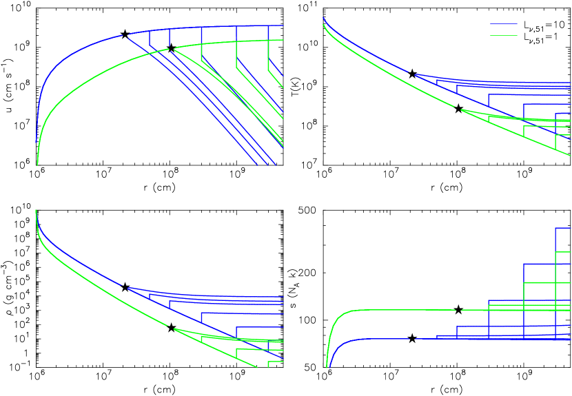
Figure 1.— Radial velocity $u$ (top left), temperature $T$ (top right), density $\rho$ (bottom left), and entropy $s$ (bottom right) in neutrino-driven winds for $M_{\mathrm{NS}}=1.4\,M_{\odot}$ as functions of radius. The neutrino luminosities are taken to be $L_{\nu,51}=10$ (blue) and 1 (green), respectively. In each $L_{\nu}$ case, the termination-shock radius is varied from the sonic radius (denoted by star) to infinity (see text).

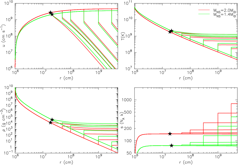
Figure 2.— Same as Figure 1, but for $M_{\mathrm{NS}}=1.4\,M_{\odot}$ (green) and $2.0\,M_{\odot}$ (red). The neutrino luminosity is taken to be $L_{\nu,51}=10$.

Figure 3.— Relations between the entropies $s_{\rm s}$ and the temperatures $T_{\rm s}$ just above the termination-shock radii $R_{\mathrm{s}}$. The neutron star masses and the neutrino luminosities are taken to be $M_{\rm NS}=1.4\,M_{\odot}$ (crosses), $2.0\,M_{\odot}$ (asterisks) and $L_{\nu,51}=10$ (solid lines), 1 (dash-dotted lines), respectively. For $M_{\mathrm{NS}}=1.4\,M_{\odot}$, $L_{\nu,51}=70$ (dashed line) is also considered as an extreme case. $R_{\mathrm{s}}$ in each $L_{\nu}$ case is varied from $R_{\mathrm{c}}$ (sonic radius, marked by circles) to 500 km, 1000 km (marked by squares), 3000 km, 10000 km (marked by triangles), and 30000 km, whenever $R_{\mathrm{s}}>R_{\mathrm{c}}$ is satisfied.

Figure 4.— Neutron-to-seed ratios $Y_{n}/Y_{h}$ at the beginning of $r$-processing ($T_{9}=2.5$) in $M_{\mathrm{NS}}=1.4\,M_{\odot}$ and $2.0\,M_{\odot}$ cases as functions of the initial electron fraction $Y_{e}$. Solid and dotted lines denote the results for $L_{\nu,51}=10$ and 1, respectively.

Figure 5.— Time variations ($t=0$ at $T_{9}=9$) of $r$ (top left), $T_{9}$ (top right), $\rho$ (bottom left), and $s$ (bottom right) for the selected shock radii $R_{\mathrm{s}}$. The neutron star mass and the neutrino luminosity are taken to be $M_{\mathrm{NS}}=1.4\,M_{\odot}$ and $L_{\nu,51}=10$, respectively.

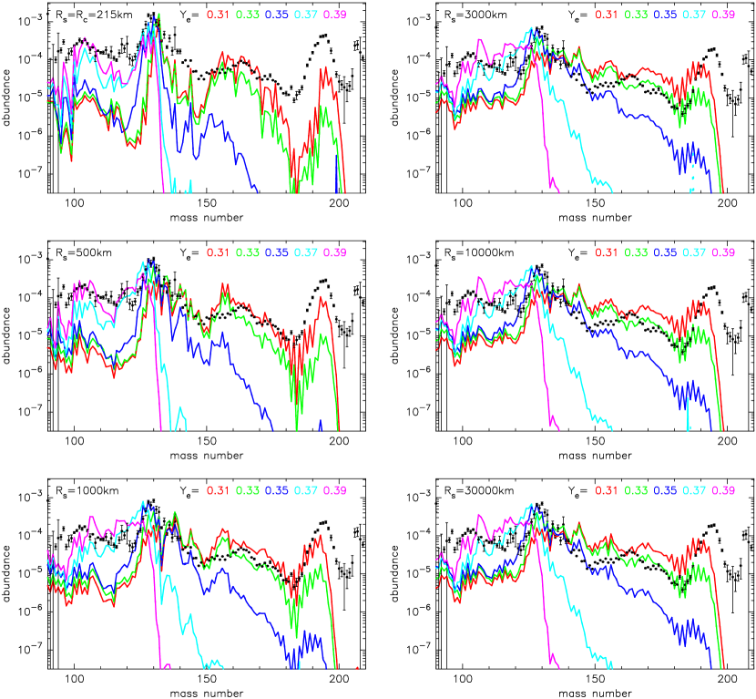
Figure 6.— Comparison of the nucleosynthetic yields (lines) for $Y_{e}=0.31$, 0.33, 0.35, 0.37, and 0.39 in the $(M_{\mathrm{NS}},L_{\nu,51})=(1.4\,M_{\odot},10)$ case with the solar $r$-process abundances (dots; Käppeler et al., 1989) as functions of mass number. The latter is shifted to match the height of the second peak ($A\approx 130$).

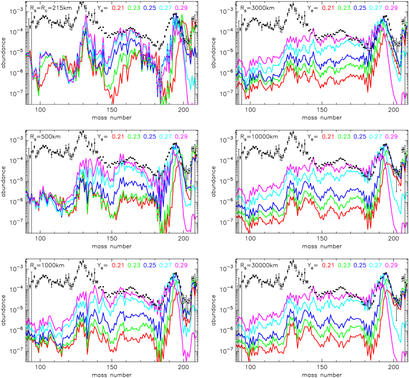
Figure 7.— Same as Figure 5, but for $Y_{e}=0.21$, 0.23, 0.25, 0.27, and 0.29. The solar $r$-process abundances are shifted to match the height of the third peak ($A\approx 195$).

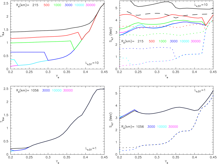
Figure 8.— Temperatures at $n$-exhaustion $T_{\mathrm{9,e}}$ (left) and nucleosynthetic paths at freezeout (in terms of neutron separation energies) $S_{\mathrm{a,f}}$ (right) for $M_{\mathrm{NS}}=1.4\,M_{\odot}$ as functions of $Y_{e}$. The termination-shock radius $R_{\mathrm{s}}$ is varied from the sonic radius up to 30000 km. Top and bottom panels show the results for $L_{\nu,51}=10$ and 1, respectively. The paths predicted from the $(n,\gamma)$-$(\gamma,n)$ equilibrium are also shown by dotted lines (right panels).

References

- Aikawa et al. (2005) Aikawa, M., Arnould, M., Goriely, S., Jorissen, A., & Takahashi, K. 2005, A&A, 441, 1195
- Arcones et al. (2007) Arcones, A., Janka, H. -Th., & Scheck, L. 2006, A&A, 467, 1227
- Arnould et al. (2007) Arnould, M., Goriely, S., & Takahashi, K. 2007, Phys. Rep., in press
- Audi et al. (2003) Audi, G., Wapstra, A. H., & Thibault, C. 2003, Nucl. Phys. A, 729, 337
- Buras et al. (2006) Buras, R., Rampp, M., Janka, H. -Th, & Kifonidis, K. 2006, A&A, 447, 1049
- Burrows et al. (1995) Burrows, A., Hayes, J., Fryxell, B. A. 1995, ApJ, 450, 830
- Burrows et al. (2007) Burrows, A., Livne, E., Dessart, L., Ott, C. D., & Murphy, J. 2007, ApJ, 655, 416
- Cardall & Fuller (1997) Cardall, C. Y. & Fuller, G. M. 1997, ApJ, 486, L111
- Cowan & Thielemann (2004) Cowan, J. J.; Thielemann, F.-K. 2004, Phys. Today, 57, 47
- Duncan et al. (1986) Duncan, R. C., Shapiro, S. L., & Wasserman, I. 1986, ApJ, 309, 141
- Freiburghaus et al. (1999) Freiburghaus, C., Rosswog, S., & Thielemann, F.-K. 1999, ApJ, 525, L121
- Fröhlich et al. (2006) Fröhlich, C., et al. 2006, ApJ, 637, 415
- Goriely & Arnould (1996) Goriely, S. & Arnould, M. 1996, A&A, 312, 327
- Goriely et al. (2005a) Goriely, S., Samyn, M., Pearson, J. M., & Onsi, M. 2005, Nucl. Phys. A, 750, 425
- Goriely et al. (2005b) Goriely, S., Demetriou, P., Janka, H. -Th., Pearson, J. M., & Samyn, M. 2005, Nucl. Phys. A, 758, 587
- Hoffman et al. (1997) Hoffman, R. D., Woosley, S. E., & Qian, Y. -Z. 1997, ApJ, 482, 951
- Ishimaru & Wanajo (1999) Ishimaru, Y. & Wanajo, S. 1999, ApJ, 511, L33
- Ishimaru et al. (2004) Ishimaru, Y., Wanajo, S., Aoki, W., & Ryan, S. G. 2004, ApJ, 600, L47
- Janka & Müller (1995) Janka, H. -T. & Müller, E. 1995, ApJ, 448, L109
- Janka & Müller (1996) Janka, H. -T. & Müller, E. 1996, A&A, 306, 167
- Käppeler et al. (1989) Käppeler, F., Beer, H., & Wisshak, K. 1989, Rep. Prog. Phys., 52, 945
- Kitaura et al. (2006) Kitaura, F. S., Janka, H. -Th., & Hillebrandt, W. 2006, A&A, 450, 345
- Kratz et al. (1993) Kratz, K. -L., Bitouzet, J., -P., Thielemann, F. -K.,Möller, P., & Pfeiffer, B. 1993, ApJ, 403, 216
- Lattimer et al. (1977) Lattimer, J. M., Mackie, F., Ravenhall, D. G., & Schramm, D. N. 1977, ApJ, 213, 225
- Mathews & Cowan (1990) Mathews, G. J. & Cowan, J. J 1990, Nature, 345, 491
- Meyer (1989) Meyer, B. S. 1989, ApJ, 343, 254
- Meyer et al. (1992) Meyer, B. S., Mathews, G. J., Howard, W. M., Woosley, S. E., & Hoffman, R. D. 1992, ApJ, 399, 656
- Ohnishi et al. (2006) Ohnishi, N., Kotake, K.,& Yamada, S. 2006, ApJ, 641, 1018
- Otsuki et al. (2000) Otsuki, K., Tagoshi, H., Kajino, T., & Wanajo, S. 2000, ApJ, 533, 424
- Qian & Woosley (1996) Qian, Y. -Z. & Woosley, S. E. 1996, ApJ, 471, 331
- Sumiyoshi et al. (2000) Sumiyoshi, K., Suzuki, H., Otsuki, K., Terasawa, M., & Yamada, S. 2000, PASJ, 52, 601
- Suzuki & Nagataki (2005) Suzuki, T. K. & Nagataki, S. 2005, ApJ, 628, 914
- Tachibana et al. (1990) Tachibana, T., Yamada, M., & Yoshida, Y. 1990, Progr. Theor. Phys., 84, 641
- Takahashi et al. (1994) Takahashi, K., Witti, J., & Janka, H. -Th. 1994, A&A, 286, 857
- Thompson et al. (2001) Thompson, T. A., Burrows, A., & Meyer, B. S. 2001, ApJ, 562, 887
- Thompson (2003) Thompson, T. A. 2003, ApJ, 585, L33
- Utsunomiya et al. (2001) Utsunomiya, H., et al. 2001, Phys. Rev. C, 63, 18801
- Wanajo et al. (2001) Wanajo, S., Kajino, T., Mathews, G. J., & Otsuki, K. 2001, ApJ, 554, 578
- Wanajo et al. (2002) Wanajo, S., Itoh, N., Ishimaru, Y., Nozawa, S., & Beers, T. C. 2002, ApJ, 577, 853
- Wanajo et al. (2004) Wanajo, S., Goriely, S., Samyn, M., & Itoh, N. 2004, ApJ, 606, 1057
- Wanajo (2006a) Wanajo, S. 2006, ApJ, 647, 1323
- Wanajo (2006b) Wanajo, S. 2006, ApJ, 650, L79
- Wanajo & Ishimaru (2006) Wanajo, S. & Ishimaru, I. 2006, Nucl. Phys. A, 777, 676
- Wanajo (2007) Wanajo, S. 2007, ApJ, submitted (astro-ph/0706.4360)
- Woosley & Hoffman (1992) Woosley, S. E. & Hoffman, R. D. 1992, ApJ, 395, 202
- Woosley et al. (1994) Woosley, S. E., Wilson, J. R., Mathews, G. J., Hoffman, R. D., & Meyer, B. S. 1994, ApJ, 433, 229