State-dependent diffusion: thermodynamic consistency and its path integral formulation

Abstract

The friction coefficient of a particle can depend on its position as it does when the particle is near a wall. We formulate the dynamics of particles with such state-dependent friction coefficients in terms of a general Langevin equation with multiplicative noise, whose evaluation requires the introduction of specific rules. Two common conventions, the Ito and the Stratonovich, provide alternative rules for evaluation of the noise, but other conventions are possible. We show the requirement that a particle’s distribution function approach the Boltzmann distribution at long times dictates that a drift term must be added to the Langevin equation. This drift term is proportional to the derivative of the diffusion coefficient times a factor that depends on the convention used to define the multiplicative noise. We explore the consequences of this result in a number examples with spatially varying diffusion coefficients. We also derive path integral representations for arbitrary interpretation of the noise, and use it in a perturbative study of correlations in a simple system.

I Introduction

Brownian motion provides a paradigm for exploring the dynamics of nonequilibrium systems, especially those that are not driven too far from equilibrium frey ; vankampen1 ; risken ; gardiner . In particular, the Langevin formulation of Brownian motion finds applications that go beyond its original purpose of describing a micron-sized particle diffusing in water. It has been extended to treat problems in dynamics of critical phenomena justin , in glassy systems cugliandolo , and even in evolutionary biology biology . Brownian motion is important for soft-matter and biological systems because they are particularly prone to thermal fluctuations frey ; lubensky , and Langevin theory is an important tool for describing their properties, such as the dynamics of molecular motors cell and the viscoelasticity of a polymer network morse .

In most applications, the diffusion coefficient is assumed to be independent of the state of the system. Yet, there are many soft-matter systems in which the diffusion coefficient is state dependent. A simple example of such a system is a particle in suspension near a wall: its friction coefficient, and hence its diffusion coefficient, depends because of hydrodynamic interactions on its distance from the wall colloidfrench , a phenomenon that affects interpretation of certain single-molecule force-extension measurements dna and that plays a crucial role in experimental verification of the fluctuation theorem in a dilute colloidal suspension near a wall seifert . Similarly, the mutual diffusion coefficient of two particles in suspension depends on their separation quake . Other examples with state-dependent diffusion include a particle diffusing in a reversible chemical polymer gel bruinsma and the dynamics of fluid membranes cai . In spite of the recent advances in digital imaging methods to probe equilibrium properties of soft matter crocker , there have been relatively few experimental studies of the dynamical properties of a physical system in which the diffusion coefficient is state dependent. This is clearly an area for further experimental exploration. Although the mathematical problem of how to treat systems with state-dependent diffusion has been studied for some time vankampen1 ; morse ; ermak ; sancho ; doi , the results of these studies have not been collected in one place to provide a clear and concise guide to both theorists and experimentalists who might use them.

In this largely expository paper, we develop a Langevin theory and its associated path integral representation for systems with state-dependent diffusion and explore its use in systems of physical interest. In accord with previous treatments vankampen1 ; risken ; morse ; colloidfrench ; ermak ; sancho ; doi , we show that a position-dependent diffusion coefficient leads naturally to multiplicative noise. This noise is the product of a state-dependent prefactor proportional to the square root of the diffusion coefficient and a state-independent dependent Gaussian white noise function, and it is meaningless without a prescription for the temporal order in which the two terms are evaluated. There are two common prescriptions or conventions for dealing with multiplicative noise: the Ito convention in which the prefactor is evaluated before the Gaussian noise and the Stratonovich convention which results when the delta-correlated white noise is obtained as a limit of a noise with a nonzero correlation time vankampen1 ; risken ; gardiner . There are, however, other conventions as we will discuss. Using general thermodynamic arguments, we show that in order for Boltzmann equilibrium to be reached a drift term proportional to the derivative of the diffusion coefficient times a factor depending on the convention for the evaluation of multiplicative noise must be added to the Langevin equation. Though this drift term has been noted before morse ; ermak ; sancho ; doi , we have found only one (recent) reference morse that specifically associate the form of the drift term with the convention for evaluating multiplicative noise. On the other hand, others claim that it is the choice of the convention that is dictated by physics colloidfrench . In particular, the authors of Ref. colloidfrench , without allowing for the possibility of the drift term, argued that neither Ito nor Stratonovich convention properly describes the dynamics of a Brownian particle with a spatially varying friction coefficient, but a third convention - what the authors called the isothermal convention, does. Incidentally, for this third convention, the drift term in our formalism vanishes. Therefore, the necessity of the drift term for enforcing thermal equilibrium is not widely known, and it is often incorrectly ignored dna . Here, we aim to provide a clear exposition for clarifying the technical issues that might have been a source of confusion in the literature.

This paper is organized as follows: in Sec. II, we first review the case of a uniform diffusion coefficient and extend it to the case of spatially varying diffusion coefficient. We discuss in depth the stochastic interpretation issues associated with multiplicative noise, we derive the Fokker-Planck equation, and we show that depending on the stochastic interpretation, an additional drift term must be added to the standard friction term in order for the system to relax to equilibrium. We also discuss how measurements of the eigenvalues and eigenfunctions of the probability that a particle is at position $x^{\prime}$ at time $t+\delta t$ given that it was at position $x$ at time $t$ can be used to obtain information about whether the diffusion coefficient is state-dependent or not. In Sec. III, we present some exactly solvable toy models that clearly illustrate the consequences of spatially varying diffusion and suggest some experimental techniques which may elucidate its role in colloidal tracking experiments. We also give numerical confirmation that the extra drift term is needed to produce equilibrium distribution. In Sec. IV, we derive and discuss the path integral formulation for a Langevin equation with a multiplicative noise, correlation functions, and perturbation theory. In Sec. V, we briefly summarize the results for multicomponent systems. Technical details are presented in the Appendices.

II Formalism in 1-d

II.1 A review for the case of a uniform diffusion coefficient

Let us first briefly review the simplest case in which a Brownian particle diffuses in space with a uniform diffusion constant vankampen1 . In the Langevin formulation of Brownian motion, the stochastic equation of motion for the particle’s position lubensky is

$$\partial_{t}x=-\Gamma\,{\partial{\cal H}\over\partial x}+g\,\eta(t),$$ (1)

where $x$ denotes the position, $\Gamma$ is the dissipative coefficient (inverse mobility), ${\cal H}$ is the Hamiltonian, and $g\,\eta(t)$ models the stochastic force arising from the rapid collisions of the water molecules with the particle. The strength of this force is set by $g$, and $\eta(t)$ is a Gaussian white noise with zero mean, $\langle\eta(t)\rangle=0$ and variance, $\langle\eta(t)\eta(t^{\prime})\rangle=\delta(t-t^{\prime})$, delta-correlated in time. The first term on the right hand side of Eq. (1) describes a dissipative process. Thus, Eq. (1) can be viewed as a balancing equation in which the first term drains the energy of the particle while the random noise pumps it back. Equation (1) neglects an inertial term that is only important at short times, typically less than $10^{-7}\,\mbox{s}$ in soft-matter systems lubensky . Thus, Eq. (1) tacitly assumes that there is a separation of time scales in which the time scale of the fast processes reflecting microscopic degrees of freedom is much shorter than the typical time scale for the random variable $x(t)$. Hence, the white noise assumption in Eq. (1).

The Fokker-Planck equation vankampen1 ; risken ; gardiner ,

$$\partial_{t}P(x,t)=\partial_{x}\left[\Gamma\,{\partial{\cal H}\over\partial x}+{1\over 2}\,g^{2}\partial_{x}\right]P(x,t),$$ (2)

which can be derived for the Langevin equation, for the probability density $P(x,t)$ that a particle is at position $x$ at time $t$ provides an alternative to Langevin equation for describing the motion of Brownian particles. It is easy to see that Eq. (2) has a steady state solution $P_{s}(x)\propto\exp[-{2\Gamma\over g^{2}}\,{\cal H}]$. If a particle is in equilibrium with a heat bath at temperature $T$, then $P_{s}(x)\propto\exp[{-\beta{\cal H}}]$ from which we conclude that $g^{2}=2\Gamma k_{B}T$. If ${\cal H}=0$, Eq. (2) reduces to a diffusion equation with diffusion constant $D=g^{2}/2$. Hence, for systems in equilibrium at temperature $T$, the diffusion constant obeys the Einstein relation $D=k_{B}T\Gamma$.

II.2 Extension to the case of state-dependent diffusion coefficient

How must the Langevin equation for a Brownian particle be modified when the friction coefficient $\Gamma$ depends on position $x(t)$, i.e., when $\Gamma$ depends on the state of the system.? Though it is generally understood vankampen1 ; morse ; ermak ; sancho ; doi ; vankampen2 that an $x$-dependent $\Gamma$ leads to an $x$-dependent $g$ and thus to multiplicative noise $g\left[x(t)\right]\eta(t)$, it is less well known that the requirements of long-time thermal equilibrium require an additional specific modification to the Langevin equation - the addition of a convention-dependent drift term. Though there are discussions in the literature of this drift term morse ; colloidfrench ; ermak ; doi , they are not very detailed, and they generally treat only a specific convention for dealing with multiplicative noise. Here we show that constraints of equilibrium require a unique drift term with each noise convention and resolve any ambiguities arnold arising from the fact that multiplicative noise can be interpreted in many ways.

Using the argument that the stochastic force is balanced by the dissipative term as in the case of a uniform dissipative coefficient above, we may reasonably postulate a Langevin equation, which trivially generalizes Eq. (1) to the case of spatially varying dissipative coefficient, to take the following form:

$$\partial_{t}x=-\Gamma(x)\,{\partial{\cal H}\over\partial x}+g(x)\eta(t),$$ (3)

where $g(x)=\sqrt{2k_{B}T\Gamma(x)}$. But we must first confront the issue of interpreting the multiplicative noise $g(x)\eta(t)$, which by itself is not defined vankampen1 ; vankampen2 . This is because the stochastic nature of $\eta(t)$ which in general consists of a series of delta-function spikes of random sign. The value of $g[x(t)]\eta(t)$ depends on whether $g[x(t)]$ is to be evaluated before a given spike, after it, or according to some other rule. It turns out, as we will show shortly, that this naive generalization of Eq. (1) to Eq. (3) is only valid for a particular interpretation of the noise.

There are a number of approaches to assigning meaning to the multiplicative noise, but they all boil down to providing rules for the evaluation of the integral

$${\cal J}(t,\Delta t)=\int_{t}^{t+\Delta t}ds\,g[\,x(s)]\,\eta(s),$$ (4)

in the limit of small $\Delta t$. If $g(x)$ and $\eta(s)$ are both continuous functions, this integral could, for arbitrary $\Delta t$, be expressed via the first integral mean-value theorem as

$${\cal J}_{\mbox{\scriptsize cont}}(t,\Delta t)=g[x(t_{i})]\int_{t}^{t+\Delta t}ds\,\,\eta(s)$$ (5)

where $t_{i}$ is a uniquely determined time in the interval $[t,t+\Delta t]$. In the limit of small $\Delta t$, this expression, Eq. (5), reduces trivially to $g[x(t)]\eta(t)\Delta t$, to lowest order in $\Delta t$. The noise $\eta(s)$ is, however, not continuous and Eq. (5) with a uniquely determined time does not apply. One can, however, use Eq. (5) to motivate a definition of ${\cal J}(t,\Delta t)$ for a stochastic $\eta(s)$. There are two commonly used conventions for defining ${\cal J}(t,\Delta t)$: the Stratonovich convention

$${\cal J}_{S}(t)=g\left[{(x(t)+x(t+\Delta t))/2}\right]\,\int_{t}^{t+\Delta t}ds\,\eta(s),$$ (6)

in which $g[x(t)]$ is evaluated at the midpoint of the interval $[x(t),x(t+\Delta t)]$ and the Ito convention

$${\cal J}_{I}(t)=g[x(t)]\,\int_{t}^{t+\Delta t}ds\,\eta(s),$$ (7)

in which $g[x(t)]$ is evaluated before any noise in the interval $(t,t+\Delta t)$ occurs. We will use a generalized definition:

$${\cal J}_{\alpha}(t,\Delta t)=g\left[\,\alpha x(t+\Delta t)+(1-\alpha)x(t)\,\right]\,\int_{t}^{t+\Delta t}ds\,\eta(s),$$ (8)

which is parameterized by a continuous variable $\alpha\in[0,1]$, that reduces to the Ito convention when $\alpha=0$, to the Stratonovich convention when $\alpha=1/2$, and to the isothermal convention of Ref. colloidfrench when $\alpha=1$.

We note in passing that in the mathematics community, the Ito calculus is most commonly used. Perhaps, this is because of the conceptual simplicity arising from the property that the noise increment $\int_{t}^{t+\Delta t}ds\,\eta(s)$ and $x(t)$ are statistically independent as implied in Eq. (7), i.e. $\langle\,g(x)\eta(t)\,\rangle=0$ oksendal . On the other hand, in the physics community, the Stratonovich interpretation is favored. In addition to the advantage that it gives rise to the ordinary rules of calculus, the Stratonovich convention also has a deeper physical origin. Since the noise term in Eq. (3) models, in a coarse-grained sense, the effects of microscopic degrees of freedom that have finite (albeit short) correlation times, this term should be physically interpreted as the limit in which these correlation times go to zero. By the Wong-Zakai theorem, this limit corresponds to a white noise that must be interpreted using the Stratonovich convention oksendal . However, Eq. (3) does not provide a correct description for systems in constact with a thermal bath at temperature $T$ for either interpretation: their associated Fokker-Planck equations do not have long-time thermal-equilibrium solutions.

To return to our main discussion, it is clear that ${\cal J}_{\alpha}(t,\Delta t)$ depends on the value of $\alpha$. Integration of Eq. (3) yields

$$\Delta x(t+\Delta t)\equiv x(t+\Delta t)-x(t)={\cal J}_{\alpha}(t,\Delta t),$$ (9)

when ${\cal H}=0$. The integral $\int_{t}^{t+\Delta t}ds\,\eta(s)$ is statistically of the order of $\sqrt{\Delta t}$, implying $\Delta x(t+\Delta t)$ is also of the order of $\sqrt{\Delta t}$. Thus, $\alpha x(t+\Delta t)+(1-\alpha)x(t)=x(t)+\alpha\Delta x(t+\Delta t)$ has a term of order $\sqrt{\Delta t}$ proportional to $\alpha$, and the order $\Delta t$ term in ${\cal J}_{\alpha}(t,\Delta t)$ depends on $\alpha$. An alternative approach to defining ${\cal J}(t,\Delta t)$ is simply to expand $g[x(s)]$ in the integrand as $g[x(s)]=g[x(t)]+[x(s)-x(t)]\,g^{\prime}[x(t)]+\cdots$. In this approach, which we outline in Appendix A, ambiguities in the interpretation of ${\cal J}(t,\Delta t)$ are resolved by specifying the value of the Heaviside unit step function, $\theta(t)$ at $t=0$. Setting $\theta(0)=\alpha$ is equivalent to using Eq. (8) for ${\cal J}(t,\Delta t)$.

The stochastic integral ${\cal J}_{\alpha}(t,\Delta t)$ depends on our convention for evaluating it, i.e. on $\alpha$. Thus, different values of $\alpha$ define different dynamics. But the requirements of thermal equilibrium should imply a unique dynamics. What is missing? To resolve this dilemma, we consider the general stochastic equation

$$\partial_{t}x=f(x)+g(x)\,\eta(t),$$ (10)

where

$$f(x)=-\Gamma(x)\,{\partial{\cal H}\over\partial x}+f_{1}(x),$$ (11)

in which we leave $f_{1}(x)$ unspecified for the moment. Eq. (10) is easily integrated using the rules we just outlined to yield

$$x(t+\Delta t)-x(t) = \int_{t}^{t+\Delta t}ds\,\left\{f[x(s)]+g[x(s)]\,\eta(s)\right\}$$ (12)

$$= f[x(t)+\alpha\Delta x]\Delta t$$

$$+ g[x(t)+\alpha\Delta x]\,\int_{t}^{t+\Delta t}ds\,\eta(s),$$

from which we obtain, to the first order in $\Delta t$,

$$\langle\Delta x\rangle = f(x_{0})\,\Delta t+\alpha g(x_{0})g^{\prime}(x_{0})\Delta t,$$ (13)

$$\langle(\Delta x)^{2}\rangle = g^{2}(x_{0})\Delta t,$$ (14)

where we set $x(t)=x_{0}$. Thus, there is a stochastic contribution, $\alpha gg^{\prime}\Delta t$, to $\langle\Delta x\rangle$ arising from the $x$ dependence of $g$ and depending on the convention for evaluating ${\cal J}(t,\Delta t)$. In equilibrium, $\langle\Delta x\rangle$ should be independent of $\alpha$. Thus, it is apparently necessary to include a contribution to $f(x)$ depending on $\alpha$.

II.3 Derivation of the Fokker-Planck Equation and Equilibrium Conditions

To determine the appropriate form of $f(x)$ and $g(x)$ to describe equilibrium systems with a spatially varying friction coefficient $\Gamma(x)$, we derive the Fokker-Planck equation for the probability density $P(x,\,t)$. The Fokker-Planck equation is most easily derived using the identity

$$P(x,t+\Delta t)=\int dx_{0}\,P(x,t+\Delta t|x_{0}\,t)P(x_{0}\,t),$$ (15)

where $P(x,t+\Delta t|x_{0}\,t)$ is the conditional probability distribution of $x$ at time $t+\Delta t$ given that it was $x_{0}$ at time $t$. It is defined by

$$P(x,t+\Delta t|x_{0}\,t)=\left\langle\delta[x-x(t+\Delta t)]\right\rangle_{x_{0},t}$$ (16)

where the average is over the random noise $\eta(s)$ and $x(t+\Delta t)$ is determined by Eq. (12) with $x(t)=x_{0}$. Taylor expanding the conditional probability around $x_{0}$ yields

$$P(x,t+\Delta t|x_{0}\,t) = \delta(x-x_{0})-\langle\Delta x\rangle\,{\partial\over\partial x}\,\delta(x-x_{0})$$

$$+ {1\over 2}\,\langle(\Delta x)^{2}\rangle\,{\partial^{2}\over\partial x^{2}}\,\delta(x-x_{0})+\cdots.$$

Then using this in Eq. (15), we obtain

$$\partial_{t}P(x,t) = {\partial\over\partial x}[-f(x)-\alpha g(x)g^{\prime}(x)]P(x,t)+{1\over 2}{\partial^{2}\over\partial x^{2}}\left[\,g^{2}(x)P(x,t)\right]$$ (17)

$$= {\partial\over\partial x}\left[\Gamma(x){\partial{\cal H}\over\partial x}-f_{1}(x)+(1-\alpha)g(x)g^{\prime}(x)+{1\over 2}\,g^{2}(x){\partial\over\partial x}\right]P(x,t).$$ (18)

For an equilibrium system, this equation must have a steady state solution with the canonical form

$$P(x,t)\sim e^{-{\cal H}/(k_{B}T)}$$ (19)

that is always approached at long times. Such a solution is guaranteed if

$$g^{2}(x) = 2k_{B}T\Gamma(x),$$ (20)

$$f_{1}(x) = (1-\alpha)g(x)g^{\prime}(x)=2(1-\alpha)k_{B}T\Gamma^{\prime}(x).\,\,\,\,\,\,\,\,\,\,$$ (21)

Thus, an additional drift term, $f_{1}(x)$, which depends on the convention for evaluating ${\cal J}(t,\Delta t)$, must be added to the standard friction term, $-\Gamma(x)\partial_{x}{\cal H}$, in the equation for $\partial_{t}x$ in order for the system to evolve to the Boltzmann distribution at long times, i.e., be consistent with thermodynamics. Note that $f_{1}(x)$ is proportional to the temperature $T$, indicating that its origin arises from random fluctuations rather from forces identified with a potential. It is clear now from Eq. (21) that if we insist on using the Langevin equation in the form of Eq. (3), we are forced to take $\alpha=1$ colloidfrench .

It is customary to express the Fokker-Planck equation in terms of the diffusion constant rather then the friction coefficient. From Eq. (14) for $\langle(\Delta x)^{2}\rangle$, we can identify $g^{2}(x)$ with the short-time diffusion constant $D(x)=2k_{B}T\Gamma(x)$. With this definition of $D(x)$ and $f_{1}(x)$ given by Eq. (21), the Fokker-Planck equation becomes

$$\partial_{t}P(x,t)={\partial\over\partial x}\,D(x)\left[\beta{\partial{\cal H}\over\partial x}+{\partial\over\partial x}\right]P(x,t),$$ (22)

where $\beta=1/(k_{B}T)$. As required, this equation is independent of $\alpha$: different conventions now give the same equilibrium condition as they should. For a free particle diffusing in spatially varying $D(x)$, ${\cal H}=0$ and Eq. (22) becomes

$$\partial_{t}P(x,t)={\partial\over\partial x}\,D(x){\partial\over\partial x}P(x,t).$$ (23)

This implies that the correct generalization of Fick’s Law for equilibrium systems with a spatially-varying diffusion coefficient is given by

$$J(x,t)=-D(x)\partial_{x}P(x,t).$$ (24)

Historically, the generalization of Fick’s law has long been debated mark . It is commonly acknowledged that Eq. (24) is right even though many derivations to the right of side of Eq. (24) seem not to be as transparent as the one given above.

II.4 Experimental probes of $D(x)$

One interesting property of Eq. (22) is that it necessarily has an eigenstate with eigenvalue zero and eigenfunction given by the equilibrium distribution the $P_{eq}(x)\propto e^{-\beta{\cal H}(x)}$. This fact is exploited by Crocker et al. crocker to measure directly the interaction between an isolated pair of colloidal particles. In these experiments, the data from tracking the motion of the particles are used to compute the conditional probability $P(x,t+\delta t|x^{\prime}t)$, which may be viewed as the Green’s function to or the inverse of the Fokker-Planck equation, Eq. (22). The equilibrium distribution is then the solution to

$$P_{eq}(x)=\int dr^{\prime}\,P(x,\,t+\delta t\,|\,x^{\prime},\,t)P_{eq}(x^{\prime}),$$ (25)

from which the interaction potential can be constructed via $U(x)=-k_{B}T\log P_{eq}(x)$.

Since the conditional probability contains all the dynamical information of the system, one could in principle characterize how the system relaxes to equilibrium by extracting the nonzero eigenvalues of Eq. (22). In particular, the Fokker-Planck equation describing a system with a state-dependent diffusion coefficient would have eigenvalues and eigenfunctions that are, in general, different from those of a system with a uniform diffusion coefficient, even though the two systems have the same Hamiltonian. Thus, in principle, one could extract the Hamiltonian from image analysis following the procedures of Crocker crocker , and solve Eq. (22) with uniform diffusion constant to obtain a set of eigenvalues (probably numerically) and compare it with experimentally measured eigenvalues, which can be extracted from the measured conditional probability. If they are different, then the diffusion coefficient is state dependent, and one needs to model the diffusion coefficient to understand the dynamical behaviors of the system. We suggest this procedure as a possible general method for experimentalists to explore the dynamics and measure the state dependent friction coefficient in, for example, hydrodynamic interactions between two spheres crocker2 , diffusion of particles in polymer solution verma , and rods in a nematic environment dogic .

III Illustrative Examples

In this section, we consider some exactly solvable toy models to illustrate some central ideas presented in the last section. In particular, we address the effects of spatial dependence in the diffusion coefficient and use numerical solution of the Langevin equation to show that equilibrium distribution is obtained only if $f_{1}(x)$, Eq. (21), is added to the standard friction term.

III.1 Diffusion of a particle near a wall

How does a diffusion coefficient acquire a spatial dependence? The simplest example is a Brownian particle diffusing near a wall located at $z=0$. Brenner brenner has shown that for $z>0$ the diffusion coefficient acquires a spatial dependence in which it is zero at the wall, rises linearly in $z$, and approaches a uniform bulk value of $D_{0}$ at large $z$ as

$${D(z)\over D_{0}}=1-{9\over 8}{a\over z}+\ldots\,\,.$$ (26)

Note the long-range component of $D(z)$ in Eq. (26), which reflects the long-ranged nature of the hydrodynamic interaction. Recently, it has been pointed out that in single molecule experiments, it is crucial to take the spatial dependence in the diffusion coefficient properly into account dna .

Rather than to treat the system with the above $D(z)$, we consider a toy model, which correctly describes diffusion close to a wall, in which $D(z)=\Lambda z$. This diffusion coefficient has another experimental realization: diffusion of a colloidal particle bounded by two parallel walls, with one of the walls slightly tilted colloidfrench . Then, the diffusion coefficient acquires a spatial dependence, approximately given by $D(z)\sim z$, for the motion of the particle parallel to the walls. In this case, the Fokker-Planck equation becomes

$$\partial_{t}P(z,t)=\Lambda{\partial\over\partial z}\,z\,{\partial\over\partial z}\,P(z,t),$$ (27)

which can be solved exactly. Let $P(z,t)=\sum_{n}c_{n}e^{-\lambda_{n}t}\psi_{n}(z),$ where $\lambda_{n}$ are a set of the eigenvalues. With the transformation $y=\sqrt{z}$, Eq. (27) can be written as

$$\psi_{n}^{{}^{\prime\prime}}(y)+{1\over y}\psi_{n}^{{}^{\prime}}(y)+{4\lambda_{n}\over\Lambda}\psi_{n}(y)=0,$$ (28)

whose solution is the Bessel function: $\psi(y)=J_{0}(ky)$, and whose eigenvalues form a continuous spectrum given by $\lambda=\Lambda k^{2}/4$. The probability distribution as a function of time can be written as

$$P(z,t)=\int_{0}^{\infty}dk\,c(k)\,e^{-\Lambda k^{2}t/4}\,J_{0}(k\sqrt{z}).$$ (29)

The probability distribution for a particle at $z=z_{0}$ at time $t=0$ evolves as

$$P(z,t)={1\over\Lambda t}\,e^{-\left[{(z+z_{0})/(\Lambda t)}\right]}I_{0}\left[\,2\sqrt{zz_{0}}/(\Lambda t)\right].$$ (30)

Unlike its counterpart for a uniform diffusion coefficient, this probability distribution is non-Gaussian. It is straightforward to calculate the moments:

$$\langle z(t)\rangle = z_{0}+\Lambda t$$

$$\langle\left[z(t)-z_{0}\right]^{2}\rangle = 2\Lambda t\,(z_{0}+\Lambda t).$$

These behaviors are very different from those of a constant diffusion. In particular, the mean-squared displacement exhibits ballistic behavior. It is interesting to observe that the second moment can be written as $\langle(\,z(t)-z_{0})^{2}\,\rangle=2\,\Lambda\langle z(t)\rangle\,t$. This suggests that in order to extract the diffusion coefficient for this simple problem, we need to know not only the second moment $\langle(\,z(t)-z_{0})^{2}\rangle$, but also the first moment $\langle z(t)\rangle$. Only for short times does the second moment reduce to $\langle(\,z(t)-z_{0})^{2}\,\rangle\sim 2\,\Lambda z_{0}\,t=2D(z_{0})t$, which is the formula commonly used to extract the diffusion coefficient. It is clearly incorrect to use this formula for times greater than $z_{0}/\Lambda$. The method we suggested at the end of the last section compliment this approach. Note also that the $\langle z(t)\rangle\sim t$ behavior has been measured in Ref. colloidfrench .

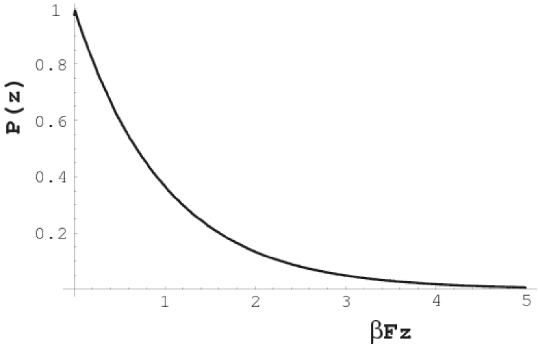
Figure 1: Stationary distribution for a particle diffusing in a diffusion coefficient $D(z)=\Lambda z$ subject to a constant force ${\bf F}=-F\,\hat{z}$. What is shown here is the numerical simulation of the Langevin equation Eq. (35); it is of the form $e^{-\beta Fz}$, as expected.

If the particle is subject to constant force $F$, like gravity, in the $-z$ direction, then the Fokker-Planck equation is

$$\partial_{t}P(z,t)=\Lambda{\partial\over\partial z}\,z\left[\beta F+{\partial\over\partial z}\right]P(z,t).$$ (31)

This problem can also be solved exactly. Let $P(z,t)=e^{-\beta Fz}\,\sum_{n}c_{n}e^{-\lambda_{n}t}\psi_{n}(z),$ we find that the eigenfunctions satisfy the Laguerre equation

$$x\psi^{{}^{\prime\prime}}+(1-x)\psi^{{}^{\prime}}+{\lambda_{n}\over\Lambda\beta F}\,\psi=0,$$ (32)

with eigenvalues $\lambda_{n}=n\Lambda\beta F$. The eigenvalue spectrum is discrete rather than continuous as it is in the case of a constant diffusion coefficient. If the particle is initially at $z_{0}$, the distribution evolves as

$$P(z,t) = {\beta F\over 1-e^{-\Lambda\beta Ft}}\exp{-\left[{\beta F(z+z_{0}e^{-\Lambda\beta Ft})\over 1-e^{-\Lambda\beta Ft}}\right]}\,$$ (33)

$$\times I_{0}\left[{2\beta F\sqrt{z_{0}ze^{-\Lambda\beta Ft}}\over 1-e^{-\Lambda\beta Ft}}\right].$$

Note that at $t\rightarrow\infty$, this distribution reaches the equilibrium distribution $P_{eq}\sim e^{-\beta Fz}$. The first two moments of $z(t)$ are

$$\langle z(t)\rangle = z_{0}e^{-\Lambda\beta Ft}+{1\over\beta F}\left(1-e^{-\Lambda\beta Ft}\right)$$

$$\langle z^{2}(t)\rangle = z_{0}^{2}e^{-2\Lambda\beta Ft}+{4z_{0}e^{-\Lambda\beta Ft}\over\beta F}(1-e^{-\Lambda\beta Ft})$$ (34)

$$+ {2\over(\beta F)^{2}}(1-e^{-\Lambda\beta Ft})^{2}.$$

Note that at long time $\langle z(t)\rangle=k_{B}T/F$ as thermal equilibrium dictates.

We numerically solve the Langevin equation corresponding this problem

$$\partial_{t}z(t)=\Lambda+\Lambda\beta Fz+\sqrt{2\Lambda z}\,\eta(t),$$ (35)

in the Ito convention numerics . Note that the first term in the right-hand side arises from the additional drift, $f_{1}(x)$ given by Eq. (21). The result for the stationary distribution is plotted in Fig. 1. Obviously, it agrees with the equilibrium distribution $P_{eq}\sim e^{-\beta Fz}$.

III.2 Diffusion of a particle bounded by two parallel walls

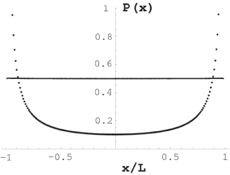
Figure 2: Stationary distribution for a particle diffusing between two walls with a diffusion coefficient $D(x)=D_{0}\left[1-(x/L)^{2}\right]$. The solid line is the numerical simulation of the Langevin equation in Eq. (39) and the dotted line is the numerical simulation of the Langevin equation without the extra $gg^{\prime}$ term.

Next, we consider the diffusion of a particle bounded by two walls, which was studied experimentally in Ref. libchaber and more recently in Ref. grier . We approximate the spatially varying diffusion coefficient of this system by $D(x)=D_{0}\left[1-(x/L)^{2}\right]$. The resulting Fokker-Planck equation is

$$\partial_{t}P(x,t)=D_{0}{\partial\over\partial x}\,\left[1-(x/L)^{2}\right]\,{\partial\over\partial x}\,P(x,t),$$ (36)

with boundary conditions that particles cannot penetrate the walls, i.e., that the flux at both walls be zero:

$$J(x,t)=D_{0}\left[1-(x/L)^{2}\right]\,{\partial\over\partial x}\,P(x,t)=0\,\,\text{at}\,\,x=\pm L.$$ (37)

Again the solution to this problem differs considerably from that with a spatially uniform diffusion coefficient. The spectrum is discrete rather than continuous with eigenvalues $\lambda_{n}=n(n+1)D/L^{2}$ ($n=1,2,...$) and the associated eigenfunctions are Legendre polynomials rather than linear combinations of plane waves. The first two moments of $x(t)$ are

$$\langle x(t)\rangle = x_{0}e^{-2D_{0}t/L^{2}}$$

$$\langle x(t)^{2}\rangle = x_{0}^{2}e^{-6D_{0}t/L^{2}}+{L^{2}\over 3}\left(1-e^{-6D_{0}t/L^{2}}\right).$$ (38)

These moments again are different from the case in which the diffusion is uniform.

We performed numerical simulation of the Langevin equation

$$\partial_{t}x=-2D_{0}x/L^{2}+\sqrt{2D_{0}(1-x^{2}/L^{2})}\,\eta(t),$$ (39)

where the first term arises from the $gg^{\prime}$ term. In Fig. 2, we plot the long time distribution (solid line) which is uniform as it should be. We also show the numerical results for the case in which we did not add the $gg^{\prime}$ (dotted line). Clearly, we get the wrong answer if we do not add the $gg^{\prime}$ term.

III.3 Diffusion constant: $D(x)=D_{0}(1+\gamma\,x^{2})$

As a final example, let us consider a free particle diffusing with $D(x)=D_{0}(1+\gamma\,x^{2})$ in the bulk. The Fokker-Planck equation is given by

$$\partial_{t}P(x,t)=D_{0}{\partial\over\partial x}\,\left[1+\gamma\,x^{2}\right]\,{\partial\over\partial x}\,P(x,t).$$ (40)

Multiplying both sides by $x^{2}$ and integrating, we find

$$\partial_{t}\langle\,x^{2}(t)\rangle=2D_{0}+6D_{0}\gamma\,\langle\,x^{2}(t)\rangle,$$ (41)

whose solution is

$$\langle\,x^{2}(t)\rangle={1\over 3\,\gamma}\left[\,\exp(6D_{0}\gamma t)-1\,\right].$$ (42)

Thus, the second moment grows exponentially with time; this peculiar behavior illustrates the dramatic effects of the noise in problems with a spatial dependent diffusion coefficient.

IV Path-integral Formulation

Path-integral formalisms provide an alternative to the Fokker-Planck and Langevin equations for the description of stochastic dynamics. They have the advantage that well-established perturbative and non-perturbative field-theoretic techniques justin ; MSR can be used to calculate the effects of nonlinearities. They also provide a convenient treatment of correlation and response functions. The path integral for a state-dependent dissipation coefficient has been derived previously either in the Stratonovich or Ito convention justin ; arnold ; phythian ; graham . In this section, we derive the path-integral for the general $\alpha$ convention, use it along with the detailed balance, a condition that any thermal systems must satisfy, to shed further insight into the additional drift term derived in Sec. II.3. We also discuss equilibrium correlation and response functions and prove the Fluctuation-dissipative theorem for state-dependent diffusion coefficient. We then set up perturbation theory for systems with a coordinate-dependent friction coefficient.

The path-integral is based on the statistics of a path $x(t)$. We discretize the path into segment $x_{i}=x(t_{i})$ with $t_{0}<t_{1}<\cdots<t_{N-1}<t_{f}$ and $\Delta t\equiv t_{n}-t_{n-1}$ small. The joint probability distribution, $P(x_{N}\,t_{N};x_{N-1}\,t_{N-1};\ldots;x_{1}\,t_{1}|x_{0}\,t_{0})$ that $x(t)$ takes on values of $x_{1}$ at time $t_{1}$, $x_{2}$ at time $t_{2}$ and so on, given that it has value of $x_{0}$ at time $t_{0}$, is then

$$P(x_{f}\,t_{f};x_{N-1}\,t_{N-1};\ldots;x_{1}\,t_{1}|x_{0}\,t_{0})$$

$$=\langle\,\delta[x_{N}-\phi(t_{N};x_{0},t_{0})]\ldots\delta[x_{1}-\phi(t_{1};x_{0},t_{0})]\,\rangle,$$

where the average is taken with respect to the noise and $\phi(t_{i};x_{i-1},t_{i-1})$ is the solution to the Langevin equation, Eq. (10), for $x(t_{i})$ given that $x(t_{i-1})=x_{i-1}$. Since the noise in Eq. (10) is delta-correlated in time, the noise in different time intervals is not correlated, and $x_{i}$ depends only on $x_{i-1}$. Thus, we can write

$$P(x_{N}\,t_{N};\ldots;x_{1}\,t_{1}|x_{0}\,t_{0})=\prod_{i=1}^{N}\langle\delta[x_{i}-\phi(t_{i};x_{i-1},t_{i-1})]\rangle.$$

The function

$$P(x_{i}\,t_{i}|x_{i-1}\,t_{i-1})=\langle\delta[x_{i}-\phi(t_{i};x_{i-1},t_{i-1})]\rangle$$ (43)

gives the conditional probability that the random variable $x(t)$ has the value $x_{i}$ at time $t_{i}$ given that it had a value $x_{i-1}$ at $t_{i-1}$. Using Eq. (43) and the identity $P(x\,t)=\int\,dx^{\prime}\,P(x\,t;x^{\prime}\,t^{\prime}),$ it is easy to see that

$$P(x_{i}\,t_{i}|x_{i-2}\,t_{i-2})=\int dx_{i-1}\,P(x_{i}\,t_{i}|x_{i-1}\,t_{i-1})$$

$$\hphantom{pppppppppp}\times P(x_{i-1}\,t_{i-1}|x_{i-2}\,t_{i-2}),$$ (44)

$$P(x_{i}\,t_{i})=\int dx_{i-1}\,P(x_{i}\,t_{i}|x_{i-1}\,t_{i-1})P(x_{i-1}\,t_{i-1}).$$ (45)

Equation (44) is the Chapman-Kolmogorov equation, which defines a Markov process vankampen1 , while Eq. (45) is just an identity, true for all stochastic processes. Note that a Markov process is completely specified if we know $P(x_{i}\,t_{i})$ and $P(x_{i}\,t_{i}|x_{i-1}\,t_{i-1})$, but they are not arbitrary because they are linked through Eqs. (44) and (45). Using Eq. (44), the conditional probability for the particle to go from $x_{0}$ at time $t_{0}$ to $x_{f}$ at time $t_{f}$ is

$$P(x_{f}\,t_{f}|x_{0}\,t_{0})=\int dx_{N-1}\ldots\int dx_{1}\,\times\,$$ (46)

$$\langle\delta[x_{f}-\phi(t_{f};x_{N-1},t_{N-1})]\rangle\ldots\langle\delta[x_{1}-\phi(t_{1};x_{0},t_{0})]\rangle.$$

This is the basic construct for the path integral. First, we have to evaluate $\langle\delta[x_{i}-\phi(t_{i};x_{i-1},t_{i-1})]\rangle$. We discretize Eq. (10) as follows:

$$x_{i}=x_{i-1}+\Delta t\,f_{i}+g_{i}\int_{t_{i-1}}^{t_{i}}dt^{\prime}\,\eta(t^{\prime}),$$ (47)

where $\Delta t=t_{i}-t_{i-1}$, $f_{i}=f[\,\alpha\,x_{i}+(1-\alpha)\,x_{i-1}]$, and $g_{i}=g[\,\alpha\,x_{i}+(1-\alpha)\,x_{i-1}]$. We next introduce the function $h(x_{i},x_{i-1})$:

$$h(x_{i},x_{i-1})={x_{i}-x_{i-1}-\Delta t\,f_{i}\over g_{i}}-\int_{t_{i-1}}^{t_{i}}dt^{\prime}\,\eta(t^{\prime}),$$ (48)

which vanishes when $x_{i}$ is the unique solution to the Eq. (47), $\phi(t_{i};x_{i-1},t_{i-1})$, i.e., $h[\phi(t_{i};x_{i-1},t_{i-1}),x_{i-1}]=0$. Using the property of the delta function

$$\delta[h(x_{i},x_{i-1})]=\left|{\partial h\over\partial x_{i}}\right|_{x_{i}=\phi(t_{i})}^{-1}\,\delta[x_{i}-\phi(t_{i})],$$

and noting that $\left|{\partial h\over\partial x_{i}}\right|_{x_{i}=\phi(t_{i})}^{-1}$ depends only on $x_{i}$ and $x_{i-1}$, which are set by the delta function and not explicitly on the noise, we have

$$\langle\delta[h(x_{i},x_{i-1})]\rangle = \left\langle\left|{\partial h\over\partial x_{i}}\right|_{x_{i}=\phi(t_{i})}^{-1}\,\delta[x_{i}-\phi(t_{i})]\right\rangle$$

$$= \left|{\partial h\over\partial x_{i}}\right|^{-1}\,\langle\delta[x_{i}-\phi(t_{i})]\rangle,$$

since for any function $q[\phi(t_{i})]$, $\langle q[\phi(t_{i})]\delta[x_{i}-\phi(t_{i})]\rangle=q(x_{i})\langle\delta[x_{i}-\phi(t_{i})]\rangle$. We can, therefore, write the conditional probability as

$$P(x_{i}t_{i}|x_{i-1}t_{i-1}) = \langle\delta[x_{i}-\phi(t_{i};x_{i-1},t_{i-1})]\rangle$$

$$= \left|{\partial h(x_{i},x_{i-1})\over\partial x_{i}}\right|\,\langle\delta[h(x_{i},x_{i-1})]\rangle,$$

with

$${\partial h\over\partial x_{i}}={1\over g_{i}}\left[{1-\alpha\Delta t\,f_{i}^{\prime}-\alpha\,{g_{i}^{\prime}\over g_{i}}\left(x_{i}-x_{i-1}-\Delta t\,f_{i}\,\right)}\right],$$

where ^′ denotes the derivative. The average over noise can be easily done with the aid of the Fourier representation of the delta function:

$$\langle\delta[h(x_{i},x_{i-1})]\rangle = \int{dk_{i}\over 2\pi}\,e^{+\imath{k_{i}\over g_{i}}(x_{i}-x_{i-1}-\Delta tf_{i})}$$

$$\times \left\langle e^{-\imath k_{i}\int_{t_{i-1}}^{t_{i}}dt^{\prime}\,\eta(t^{\prime})}\right\rangle,$$

$$= \int{dk_{i}\over 2\pi}\,e^{+\imath{k_{i}\over g_{i}}(x_{i}-x_{i-1}-\Delta tf_{i})-{1\over 2}k_{i}^{2}\Delta t},$$

where we have made use of the fact that $\int_{t_{i-1}}^{t_{i}}dt^{\prime}\,\eta(t^{\prime})$ is a zero-mean Gaussian random variable with variance $\Delta t$. Putting these results together, we can express $P(x_{i}t_{i}|x_{i-1}t_{i-1})$ as

$$P(x_{i}t_{i}|x_{i-1}t_{i-1})=\int{dk_{i}\over 2\pi g_{i}}\,e^{+\imath{k_{i}\over g_{i}}(x_{i}-x_{i-1}-\Delta tf_{i})-{1\over 2}k_{i}^{2}\Delta t}$$

$$\phantom{pppp}\times\left[1-\alpha\Delta t\,f_{i}^{\prime}-\alpha\,{g_{i}^{\prime}\over g_{i}}\left(x_{i}-x_{i-1}-\Delta t\,f_{i}\,\right)\right].\,$$ (49)

Next, in order to derive the path integral which is of the form $\sim e^{-{\cal S}}$, we need to “exponentiate” the bracket term in Eq. (49) and keep all the terms that are of order of $\Delta t$ in the exponential. However, we cannot simply exponentiate the third term in the bracket because this term contains $\Delta x_{i}\equiv x_{i}-x_{i-1}$, which is of order of $\sqrt{\Delta t}$. This is noted in Ref. arnold , where the author derives the path integral for the Stratonovich convention, and circumvents this difficulty by keeping the second order term in $\Delta x$ in the exponential and replacing this term with its average value. Although the final expression is correct, that derivation might be inconsistent with the concept of path integral since that derivation is valid only in the mean-squared sense instead of for all paths, as required by the path integral. Here, we provide an alternative derivation that is valid for each path. First, we note that the last term in the bracket can be written as

$$-\int{dk_{i}\over 2\pi g_{i}}\,\left[\,\alpha{g_{i}^{\prime}\over g_{i}}\left(\Delta x_{i}-\Delta t\,f_{i}\,\right)\right]\,e^{+\imath{k_{i}\over g_{i}}(\Delta x_{i}-\Delta tf_{i})-{1\over 2}k_{i}^{2}\Delta t} = -\,\alpha g_{i}^{\prime}\int{dk_{i}\over 2\pi g_{i}}\,e^{-{1\over 2}k_{i}^{2}\Delta t}\left(-\imath{\partial\over\partial k_{i}}\right)e^{+\imath{k_{i}\over g_{i}}(\Delta x_{i}-\Delta tf_{i})}$$ (50)

$$= +\,\alpha g_{i}^{\prime}\int{dk_{i}\over 2\pi g_{i}}\left[\,\imath k_{i}\Delta t\,\right]e^{+\imath{k_{i}\over g_{i}}(\Delta x_{i}-\Delta tf_{i})-{1\over 2}k_{i}^{2}\Delta t},$$

where the last line explicitly of order of $\Delta t$ and can, therefore, be exponentiated without incurring any error to the first order in $\Delta t$. Returning to the conditional probability, we have

$$P(x_{i}t_{i}|x_{i-1}t_{i-1}) = \int{dk_{i}\over 2\pi g_{i}}\,e^{+\imath{k_{i}\over g_{i}}(\Delta x_{i}-\Delta tf_{i})-{1\over 2}k_{i}^{2}\Delta t}\left[\,1-\alpha\Delta t\,f_{i}^{\prime}+\imath\alpha\Delta tk_{i}g_{i}^{\prime}\,\right]$$ (51)

$$= \int{dk_{i}\over 2\pi g_{i}}\,e^{+\imath{k_{i}\over g_{i}}(\Delta x_{i}-\Delta tf_{i}+\alpha\Delta tg_{i}g_{i}^{\prime})-{1\over 2}k_{i}^{2}\Delta t-\alpha\Delta t\,f_{i}^{\prime}}$$ (52)

$$= {1\over\sqrt{2\pi\Delta t}\,g_{i}}\,e^{-{\Delta t\over 2g_{i}^{2}}\left[{\Delta x_{i}\over\Delta t}-f_{i}+\alpha g_{i}g_{i}^{\prime}\right]^{2}-\alpha\Delta tf_{i}^{\prime}},$$ (53)

where the last line is valid to the first order in $\Delta t$. It should be noted that the Fokker-Planck equation, Eq. (17), can also be derived using Eq. (53) and the identity of Eq. (45). This is done in the Sec. IV.1. Returning to Eq. (46), we have

$$P(x_{f}\,t_{f}|x_{0}\,t_{0}) = \int{dx_{1}\over\sqrt{2\pi\Delta t}g_{1}}\ldots\int{dx_{N-1}\over\sqrt{2\pi\Delta t}g_{N-1}}{1\over\sqrt{2\pi\Delta t}g_{N}}e^{-\sum_{i}{\Delta t\over 2g_{i}^{2}}\left[{x_{i}-x_{i-1}\over\Delta t}-f_{i}+\alpha g_{i}^{\prime}g_{i}\right]^{2}-\sum_{i}\alpha\Delta tf_{i}^{\prime}}$$ (54)

$$= \int_{x_{0}}^{x_{f}}{\cal D}x\,e^{-\int_{t_{0}}^{t_{f}}dt\,\left\{{1\over 2g(x)^{2}}\left[\partial_{t}x-f(x)+\alpha\,g(x)\,g^{\prime}(x)\right]^{2}+\alpha f^{\prime}(x)\right\}}=\int_{x_{0}}^{x_{f}}{\cal D}x\,e^{-{\cal S}},$$ (55)

with ${\cal D}x\equiv\prod_{i=1}^{N}{dx_{i}\over\sqrt{2\pi\Delta t}g_{i}}$, and the action given by

$${\cal S}=\int_{t_{0}}^{t_{f}}dt\left\{{1\over 2g(x)^{2}}\left[\partial_{t}x-f(x)+\alpha\,g(x)\,g^{\prime}(x)\right]^{2}+\alpha f^{\prime}(x)\right\},$$ (56)

where we have taken the formal limit of by letting $N\rightarrow\infty$ and $\Delta t\rightarrow 0$. Note the extra terms in the ${\cal S}$ coming from the Jacobian $\left|\partial h/\partial x_{i}\right|$; they are needed in order to ensure that $\int dx_{f}P(x_{f}\,t_{f}|x_{0}\,t_{0})=1$. This can be demonstrated by explicit, but tedious, calculation for general $\alpha$ (see Appendix B). From Eq. (56), it is clear that the Ito convention with $\alpha=0$ is the simplest to deal with. Another particular useful form of the path integral is obtained using the Hubbard-Stratonovich transformation, which linearizes the quadratic term

$$P(x_{f}\,t_{f}|x_{0}\,t_{0})=\int{\cal D}y\,\int_{x_{0}}^{x_{f}}{\cal D}x\,\exp{-\int_{t_{0}}^{t_{f}}dt\,\left\{{g(x)^{2}\over 2}\,y^{2}(t)-\imath y(t)\left[\partial_{t}x-f(x)+\alpha\,g(x)\,g^{\prime}(x)\right]+\alpha f^{\prime}(x)\right\}},$$ (57)

where the measure now is $\int{\cal D}y\,\int_{x_{0}}^{x_{f}}{\cal D}x=\int{dy_{N}\over 2\pi}\ldots\int{dy_{1}\over 2\pi}\int dx_{N-1}\ldots\int dx_{1}$. This result could, of course, also have been obtained directly by substituting $k_{i}\equiv g_{i}\,y_{i}$ in Eq. (52) and taking the continuum limit. Note that in the discretized version of Eq. (57), $y_{n}$ is associated with time $t^{*}_{n}=\alpha\,t_{n}+(1+\alpha)\,t_{n-1}$. This form of the path integral is closely related to the MSR formalism MSR to calculate response and correlation functions. This will be explored in Sec. IV.2.

It is interesting to see how the additional drift tern $f_{1}(x)$ in the Langevin Equation [Eq. (11)] arises from the constraints that equilibrium statistical mechanics impose on the path integral formulation janssen . Thermal systems must obey detailed balance which states that

$$P(x_{f}\,t_{f}|x_{0}\,t_{0})P_{eq}(x_{0})=P(x_{0}\,t_{f}|x_{f}\,t_{0})P_{eq}(x_{f}).$$ (58)

The equilibrium distribution has the form $P_{eq}(x)=\exp{-[\beta\,{\cal H}(x)]}$, and $P(x_{0}\,t_{f}|x_{f}\,t_{0})$ is the conditional probability for the reversed path, i.e., for $\bar{x}(t)=x(-t)$. It turns out that the Stratonovich convention is the simplest for the discussion of time-reversal properties not only because it obeys the ordinary rule of differential calculus, but also because it has the property that the forward and backward paths are evaluated at the same points. We will employ the Stratonovich convention below. First, we note that

$${P_{eq}(x_{f})\over P_{eq}(x_{0})} = \exp{-[\beta{\cal H}(x_{f})-\beta{\cal H}(x_{0})]}$$ (59)

$$= \exp{-\left[\int_{t_{0}}^{t_{f}}dt\,(\partial_{t}x)\,{\partial\beta{\cal H}(x)\over\partial x}\right]},$$

and that $P(x_{0}\,t_{f}|x_{f}\,t_{0})$ can be obtained simply by noting that the path associated with this distribution is the time-reversal path of $P(x_{f}\,t_{f}|x_{0}\,t_{0})$, which can be written as

$$P(x_{0}\,t_{f}|x_{f}\,t_{0}) = \int{\cal D}\tilde{y}\,\int_{x_{0}}^{x_{f}}{\cal D}x\,$$

$$\times \,e^{-\int_{t_{0}}^{t_{f}}dt\,[{g^{2}\over 2}\,\tilde{y}^{2}+\imath\tilde{y}\left[\partial_{t}x+f-{1\over 2}gg^{\prime}\right]+{1\over 2}f^{\prime}]}.$$

Now, using Eqs. (58), (59), and (IV) and comparing this term by term with exponential in Eq. (57) [in the Stratonovich convention $\alpha=1/2\,$], we see that

$$\imath\tilde{y}(t) = -\left[\imath y(t)+{\partial\beta{\cal H}(x)\over\partial x}\right],$$ (61)

$$f(x) = {1\over 2}\,g(x)g^{\prime}(x)-{g^{2}(x)\over 2}\,{\partial\beta{\cal H}(x)\over\partial x}.$$ (62)

The first term in Eq. (62) is identical to Eq. (21) in the Stratonovich interpretation. The second term is the standard frictional term, from which we identify the dissipation coefficient as $\Gamma(x)=\beta g^{2}(x)/2$, which is the Einstein relation. This derivation again demonstrates that equilibrium distribution is the only physics needed to fix $f(x)$ for a given stochastic interpretation.

IV.1 Derivation of the Fokker-Planck Equation from the Path-integral

In this subsection, we derive the Fokker-Planck equation directly from the conditional probability Eq. (53), thereby establishing the equivalence of the path integral formulation and the Fokker-Planck equation for general $\alpha$. Let us rewrite the conditional probability, Eq. (52), where we set $x=x_{i}$, $t=t_{i}$, $x^{\prime}=x_{i-1}$, $t^{\prime}=t_{i-1}$, and $k_{i}\equiv g_{i}\,y_{i}$:

$$P(x\,t\,|x^{\prime}\,t^{\prime})\hphantom{ppppppppppppppppppppppppppppppppp}$$

$$=\int{dy_{i}\over 2\pi}\,e^{-\Delta t\,[{g_{i}^{2}\over 2}\,y_{i}^{2}-\imath y_{i}\left[{\Delta x_{i}\over\Delta t}-f_{i}+\alpha g_{i}g^{\prime}_{i}\right]+\alpha f^{\prime}_{i}]},$$

$$=\int{dy_{i}\over 2\pi}\,e^{-\Delta t\,{\cal A}_{i}+\imath y_{i}\Delta x_{i}},$$ (63)

where

$${\cal A}_{i}[x_{i},x_{i-1};y_{i}]\equiv{g_{i}^{2}\over 2}\,y_{i}^{2}+\imath y_{i}\left[f_{i}-\alpha g_{i}g^{\prime}_{i}\right]+\alpha f^{\prime}_{i},$$ (64)

$\Delta x_{i}=x-x^{\prime}$, and $\Delta t=t-t^{\prime}$. Our aim is to calculate

$$P(x,t)=\int dx^{\prime}\,P(x\,t\,|x^{\prime}\,t^{\prime})\,P(x^{\prime},t^{\prime}),$$ (65)

to first order in $\Delta t$. Expanding $P(x^{\prime},t)$

$$P(x^{\prime},t^{\prime})=P(x-\Delta x_{i},t^{\prime})$$

$$\hphantom{pp}=P(x,t^{\prime})-\Delta x_{i}\,{\partial\over\partial x}\,P(x,t^{\prime})+{(\Delta x_{i})^{2}\over 2}{\partial^{2}\over\partial x^{2}}P(x,t^{\prime}),$$

and putting this back to Eq. (65), we find that it can cast in the form

$${P(x,t)-P(x,t^{\prime})\over\Delta t} = \alpha(x)\,P(x,t^{\prime})+\beta(x)\,{\partial\over\partial x}P(x,t^{\prime})$$ (66)

$$+ \gamma(x)\,{\partial^{2}\over\partial x^{2}}P(x,t^{\prime}),$$

where $\alpha(x)\equiv\lim_{\Delta t\rightarrow 0}\,{\left[\,{\cal I}_{0}(x)-1\,\right]/\Delta t}$, $\beta(x)\equiv-\lim_{\Delta t\rightarrow 0}\,{{\cal I}_{1}(x)/\Delta t}$, and $\gamma(x)\equiv\lim_{\Delta t\rightarrow 0}\,{{\cal I}_{2}(x)/(2\,\Delta t)}$. The main task is to evaluate integral of the form

$${\cal I}_{m}(x)\equiv\int{dy_{i}\over 2\pi}\int d\Delta x_{i}\,(\Delta x_{i})^{m}\,Q(x,\Delta x_{i};y_{i})\,e^{iy_{i}\Delta x},$$ (67)

where

$$Q(x,\Delta x_{i};y_{i}) = e^{-\Delta t\,{\cal A}_{i}[x,x^{\prime};y_{i}]},$$ (68)

$$= \sum_{k}{(\Delta x_{i})^{k}\over k!}\,\left.{\partial^{k}\over\partial\Delta x_{i}^{k}}\,Q(x,\Delta x_{i};y_{i})\right|_{\Delta x_{i}=0},$$

where in the last line, we have Taylor expanded the function $Q(x,\Delta x_{i};y_{i})$. It is easy to see that

$$\int d\Delta x_{i}\,(\Delta x_{i})^{m}\,e^{iy_{i}\Delta x_{i}}=2\pi(-\imath)^{m}{\partial^{m}\over\partial y_{i}^{m}}\,\delta(y_{i}),$$ (69)

and therefore

$${\cal I}_{m}(x)=\sum_{k}{(\imath)^{k+m}\over k!}\left.{\partial^{m+k}\over\partial y_{i}^{m+k}}\,Q^{(k)}(x,0;y_{i})\right|_{y_{i}=0},$$ (70)

where $Q^{(k)}(x,0;y_{i})\equiv\left.{\partial^{k}Q(x,\Delta x_{i};y)/\partial\Delta x_{i}^{k}}\right|_{\Delta x_{i}=0}$. Using Eq. (70), it is straightforward to compute ${\cal I}_{m}(x)$ to the first order in $\Delta t$; we obtain

$${\cal I}_{0}(x) = 1-f^{\prime}(x)\,\Delta t$$ (71)

$$+ (1-\alpha)\,\left\{[g^{\prime}(x)]^{2}+g(x)g^{\prime\prime}(x)\right\}\,\Delta t,$$

$${\cal I}_{1}(x) = \left[\,f(x)-(2-\alpha)g(x)g^{\prime}(x)\,\right]\Delta t,$$ (72)

$${\cal I}_{2}(x) = g^{2}(x)\,\Delta t,$$ (73)

with vanishing higher order terms, i.e. ${\cal I}_{n}(x)=0$ for $n\geq 3$. Therefore, we have

$$\alpha(x) = -f^{\prime}(x)+(1-\alpha)\left[g^{\prime}(x)^{2}+g(x)g^{\prime\prime}(x)\right],$$ (74)

$$\beta(x) = -f(x)+(2-\alpha)g(x)g^{\prime}(x),$$ (75)

$$\gamma(x) = {1\over 2}\,g(x)^{2}.$$ (76)

This is equivalent to the Mori expansion risken . It is clear that with these coefficients Eq. (66) becomes Eq. (17), the Fokker-Planck equation.

IV.2 Correlation, Response functions, and Fluctuation-Dissipation Theorem

One of the advantages of the particular form of the path integral in Eq. (57) is that correlation and response functions can be computed conveniently from it. The average of any functional ${\cal O}[x(t),y(t)]$ of $x(t)$ and $y(t)$ at fixed $x_{0}$ is given by

$$\left\langle{\cal O}[x(t),y(t)]\right\rangle_{x_{0}}=\int{\cal D}y\,\int_{x_{0}}{\cal D}x\,{\cal O}[x(t),y(t)]\,e^{-{\cal S}}.$$ (77)

In particular, the two-point correlation function is

$$\langle\,x(t_{1})\,x(t_{2})\,\rangle_{x_{0}}=\int{\cal D}y\,\int_{x_{0}}{\cal D}x\,x(t_{1})x(t_{2})\,e^{-{\cal S}},$$ (78)

and the propagator function

$$G(t_{2},t_{1}) \equiv \langle\,x(t_{2})\,[-\imath y(t_{1})]\,\rangle_{x_{0}}$$ (79)

$$= \int{\cal D}y\,\int_{x_{0}}{\cal D}x\,x(t_{2})[-\imath y(t_{1})]\,e^{-{\cal S}}.$$

Physically, the propagator describes the response of the system to a delta perturbation. One of the nice features of the propagator function, which is useful in perturbative expansions, is that causality is automatically built-in, i.e. $G(t,t^{\prime})=0$ if $t<t^{\prime}$. To see this, we go back to the discretized form of the path integral and write $G(t,t^{\prime})$ as

$$G(t_{m},t_{n}) = \int{dy_{N}\over 2\pi}\ldots\int{dy_{1}\over 2\pi}\int dx_{N}\ldots\int dx_{1}\,$$ (80)

$$\times x_{m}\,[-\imath y_{n}]\,e^{-\sum_{i}\Delta t\,{\cal A}_{i}+\sum_{i}\imath y_{i}\Delta x_{i}},$$

where ${\cal A}_{i}[x_{i},x_{i-1};y_{i}]$ is defined in Eq. (64). First, let us consider $t_{n}>t_{m}$; each pair of the integrals $\int{dy_{i}\over 2\pi}\int dx_{i}$ in Eq. (80) gives $1$ for $i>n$. When integrating over $x_{n}$, we make use the following identity

$$\int dx_{n}\,Q[x_{n-1},\Delta x_{n};y_{n}]e^{+\imath y_{n}\Delta x_{n}}\hphantom{ppppppppppp}$$

$$=\sum_{k}{(\imath)^{k}\,Q^{(k)}[x_{n-1},0,y_{n}]\over k!}\,{\partial^{k}\over\partial y_{n}^{k}}\,\delta(y_{n}),$$ (81)

which gives zero when integrating $y_{n}$. Thus, we have shown $\langle x_{m}[-\imath y_{n}]\rangle_{x_{0}}=0$ for all $n>m$. Now, suppose $m=n$, one can show that using the above identity, $\langle x_{n}[-\imath y_{n}]\rangle_{x_{0}}=1$. Clearly, $\langle x_{m}[-\imath y_{n}]\rangle_{x_{0}}\neq 0$, if $m>n$. Thus, we have shown how the path integral enforces causality, i.e.  $G(t,t^{\prime})=0$ if $t<t^{\prime}$, and $G(t,t^{\prime})\neq 0$ if $t>t^{\prime}$. However, there is a subtle point about the value of $G(t,t)$ in the continuum limit, which has to be consistent with the $\alpha$-convention. The simplest way do this is to note that since $y_{n}$ is really associated with time at $t^{*}_{n}=\alpha\,t_{n}+(1-\alpha)\,t_{n-1}$, we have to evaluate

$$G(t,t) \equiv \langle\,x(t^{*}_{n})[-\imath y_{n}]\rangle_{x_{0}}$$

$$= \langle\,[\,\alpha\,x_{n}+(1-\alpha)\,x_{n-1}](-\imath y_{n})\,\rangle_{x_{0}}=\alpha.$$

Now, we specialize to a system near equilibrium, and we investigate how the path integral describes properties such as the Fluctuation-Dissipation Theorem. The equilibrium average of any function ${\cal O}[x(t),y(t)]$ of $x(t)$ and $y(t)$ is defined as

$$\left\langle{\cal O}[x(t),y(t)]\right\rangle_{eq}=\int{\cal D}y\,\int{\cal D}x\,{\cal O}[x(t),y(t)]\,e^{-{\cal S}}P_{eq}(x_{0}).$$ (82)

Note that equilibrium averages are independent of $\alpha$, provided that we add the additional drift $f_{1}(x)$. When the system is under a time-dependent physical force $h(t)$, the total Hamiltonian is ${\cal H}_{T}={\cal H}_{0}(x)-x(t)h(t),$ so that

$$f(x,t) = (1-\alpha)gg^{\prime}-\Gamma(x){\partial{\cal H}_{T}\over\partial x}=f_{0}(x)+\Gamma(x)h(t),$$

$$f_{0}(x) = (1-\alpha)gg^{\prime}-\Gamma(x){\partial{\cal H}_{0}\over\partial x}.$$

Therefore, we have

$$\left.{\delta\langle x(t)\rangle\over\delta h(t^{\prime})}\right|_{h(t)=0} = {1\over 2k_{B}T}\left\langle\,x(t)\left\{-\imath y(t^{\prime})\,g[x(t^{\prime})]^{2}\right\}\right\rangle_{eq}$$

$$- {\alpha\over k_{B}T}\left\langle\,x(t)g[x(t^{\prime})]g^{\prime}[x(t^{\prime})]\right\rangle_{eq}$$

$$\equiv {\cal\chi}_{xx}(t,t^{\prime}).$$

We observe that the response $\chi_{xx}(t,t^{\prime})$ to a physical forces and the propagator $G(t,t^{\prime})$ defined in Eq. (79) are different, although they are proportional to each other for the case of uniform diffusion constant. In particular, there is an additional term arising from the normalization factor $f^{\prime}$ in the action and it is absent when the diffusion constant is spatially uniform. By integration by parts, the first term in the bracket can be evaluated to be

$$\langle\,x(t)\left\{-\imath y(t^{\prime})\,g[x(t^{\prime})]^{2}\right\}\rangle_{eq}\hphantom{\partial_{t^{\prime}}x(t^{\prime})-f_{0}[x(t^{\prime})]\partial_{t^{\prime}}x(t^{\prime})++}$$

$$=\langle\,x(t)\left\{\partial_{t^{\prime}}x(t^{\prime})-f_{0}[x(t^{\prime})]+\alpha g[x(t^{\prime})]g^{\prime}[x(t^{\prime})]\right\}\rangle_{eq}.$$

Therefore, the physical response function is

$${\cal\chi}_{xx}(t,t^{\prime})={1\over 2k_{B}T}\,\left\langle\,x(t)\left\{\partial_{t^{\prime}}x(t^{\prime})-{\cal B}[x(t^{\prime})]\right\}\right\rangle_{eq},$$ (84)

where ${\cal B}(x)\equiv gg^{\prime}-\Gamma(x){\partial{\cal H}_{0}/\partial x}$. Note that the physical response function is independent of $\alpha$, as it should be; note also the a drift proportional to $gg^{\prime}$ arises from spatial varying diffusion constant. To proceed further, we note that as a consequence of the detailed balance condition, Eq. (58), the equilibrium correlation function is symmetric with respect to exchange of $t\leftrightarrow t^{\prime}$:

$$\left\langle{\cal O}_{1}[x(t)]{\cal O}_{2}[x(t^{\prime})]\right\rangle_{eq}=\left\langle{\cal O}_{1}[x(t^{\prime})]{\cal O}_{2}[x(t)]\right\rangle_{eq}.$$

Applying this to Eq. (84) and subtracting the results, we have

$$\left[\partial_{t}-\partial_{t^{\prime}}\right]\left\langle x(t)x(t^{\prime})\right\rangle_{eq}=2k_{B}T\left[{\cal\chi}_{xx}(t^{\prime},t)-{\cal\chi}_{xx}(t,t^{\prime})\right].$$

Since the correlation function is time translational invariant, we must have $\partial_{t^{\prime}}\left\langle x(t)x(t^{\prime})\right\rangle_{eq}=-\partial_{t}\left\langle x(t)x(t^{\prime})\right\rangle_{eq}$. Thus,

$$\partial_{t}\left\langle x(t)x(t^{\prime})\right\rangle_{eq}=-k_{B}T\,\left[{\cal\chi}_{xx}(t,t^{\prime})-{\cal\chi}_{xx}(t^{\prime},t)\right].$$

This is the Fluctuation-Dissipation Theorem. To put it in a more traditional form, we note that ${\cal\chi}_{xx}(t^{\prime},t)=0$ when $t>t^{\prime}$, and we can write

$${\cal\chi}_{xx}(t-t^{\prime})=-{1\over k_{B}T}\,\partial_{t}\left\langle x(t)x(t^{\prime})\right\rangle_{eq}\,\theta(t-t^{\prime}),$$

where $\theta(t)$ is the Heaviside unit step function. The Fourier transform of the response function is given by

$$\left\langle x(\omega)x(-\omega)\right\rangle_{eq}={2k_{B}T\over\omega}\,\mbox{Im}\,{\cal\chi}_{xx}(\omega),$$ (85)

which is of the form that is commonly quoted in the literature.

IV.3 Perturbation Theory

One of the advantages of the path integral formulation of stochastic dynamics is that it is by construction a field theory that facilitates systematic perturbative calculation of correlation functions. In particular, for systems with state-dependent dissipative coefficients, the resulting Langevin equation is generally nonlinear, and perturbation theory is a convenient way to derive the mode-coupling theory reichman . Thus, in this subsection, we set up the perturbation theory for a systematic calculation of correlation and response functions in the deviation of the diffusion coefficient from spatial uniformity. First, we need to set up the generating functional. Note that $P_{eq}(x_{0})$ satisfies

$$P_{eq}(x)=\int dx_{s}\,P(x\,t\,|x_{s}\,t_{s})P_{eq}(x_{s}),$$ (86)

which implies that

$$P_{eq}(x)=\lim_{t_{s}\rightarrow-\infty}\,P(x\,t\,|x_{s}\,t_{s}).$$ (87)

Thus, the equilibrium averages can be written as

$$\left\langle{\cal O}[x(t),y(t)]\right\rangle_{eq} = \int{\cal D}y\,\int{\cal D}x\,{\cal O}[x(t),y(t)]\,e^{-{\cal S}}P_{eq}(x_{0})$$

$$= \int{\cal D}y\,\int{\cal D}x\,{\cal O}[x(t),y(t)]\,e^{-{\cal S}},$$

where in the last line, the limit of the time integration in the action ${\cal S}$ is extended to $-\infty$ to $\infty$. This allows us to define the generating function for equilibrium averages by

$${\cal Z}[F,\tilde{F}]=\int{\cal D}y\,\int{\cal D}x\,e^{-{\cal S}+\int dt[x(t)F(t)-\imath y(t)\tilde{F}(t)]}.$$ (88)

The correlation functions and the propagator are simply functional derivatives of ${\cal Z}$. This sets up the MSR perturbation scheme MSR that allows the immediate application of all of the powerful techniques of field theory, including the renormalization group, to nonlinear stochastic problems. It is customary to introduce the variables $\hat{x}(t)\equiv-\imath y(t)$. Note that in the perturbation expansion, all the $\alpha$ dependent terms cancel provided that we use $\langle x(t)\hat{x}(t)\rangle_{0}=\alpha$ (see Appendix C). Therefore, it is convenient to use $\alpha=0$ at the outset.

As an informative model calculation, we explore the problem in which a particle diffusing with $D(x)=D_{0}\left(1+\gamma\,x^{2}\right)$ confined in a harmonic potential, ${\cal H}=kx^{2}/2$. If the confining potential is turned off, this problem is exactly solvable, as shown in Sec. III.3. It can also be solved exactly when $\gamma=0$ but not when $\gamma\neq 0$, and a perturbative expansion in $\gamma$ is useful. The goal of this exercise is to compute the propagator $\langle x\hat{x}\rangle$ and the correlation function $\langle xx\rangle$ separately and to check that the Fluctuation-Dissipation theorem is satisfied. For simplicity, we work in the Ito convention (see Appendix C for general $\alpha$), and set $k_{B}=1$. According to the formalism, we have

$$f(x) = g(x)g^{\prime}(x)-\Gamma(x){\partial{\cal H}\over\partial x}$$ (89)

$$= -\Gamma_{0}(k-2\gamma T)\,x-\Gamma_{0}k\gamma x^{3}.$$

It should be pointed out that from Eq. (89) one might at first sight conclude that there is a broken-symmetry state, when $k<2\gamma T$, with $\langle x\rangle\neq 0$. But we know that this cannot happen because the stationary distribution is in fact the Boltzmann distribution. Therefore, one could get the wrong physics if one only looks at “classical” trajectory, i.e. solution to $\partial_{t}x=f(x)$, which maximizes the action ${\cal S}$ in the Ito convention. This shows again the importance of noise in these problems.

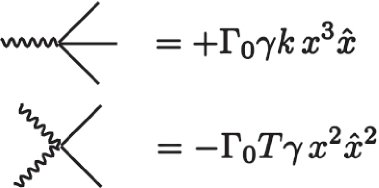
Figure 3: The two vertices corresponding to Eq. (91) for a particle diffusing in a spatially varying diffusion coefficient given by $D(x)=D_{0}(1+\gamma\,x^{2})$, and confined in a harmonic potential.

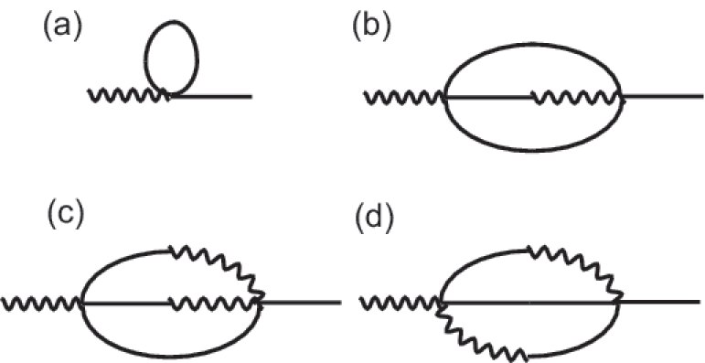
Figure 4: Diagrams that contribute to the self-energy $\Sigma(\omega)$. Note that diagram $d$ is identically zero.

The unperturbed and perturbing actions are

$${\cal S}_{0} = \int dt\left[-D_{0}\hat{x}^{2}+\hat{x}\left(\partial_{t}x+\Gamma_{0}k^{\prime}x\right)\right]$$ (90)

$${\cal S}_{I} = \Gamma_{0}\gamma\int dt\left[k\,x^{3}\hat{x}-T\,x^{2}\hat{x}^{2}\right],$$ (91)

where $k^{\prime}\equiv k-2\gamma T$. Introducing the state vector $x_{\alpha}=(\hat{x},x)$, we can write ${\cal S}_{0}$ as

$${\cal S}_{0}={1\over 2}\int{d\omega\over 2\pi}x_{\alpha}(\omega)G^{-1}_{\alpha\beta}(\omega)x_{\beta}(-\omega),$$ (92)

where

$$G^{0\,-1}_{\alpha\beta}(\omega)=\left(\begin{array}[]{cc}-2D_{0}&-\imath\omega+\Gamma_{0}k^{\prime}\\ \imath\omega+\Gamma_{0}k^{\prime}&0\\ \end{array}\right),$$

and thus

$$G^{0}_{\alpha\beta}(\omega)=\left(\begin{array}[]{cc}0&{1\over\imath\omega+\Gamma_{0}k^{\prime}}\\ {1\over-\imath\omega+\Gamma_{0}k^{\prime}}&{2D_{0}\over|-\imath\omega+\Gamma_{0}k^{\prime}|^{2}}\\ \end{array}\right),$$

from which we can read off the bare propagator and the zeroth-order correlation function:

$$\langle\hat{x}(\omega)\hat{x}(\omega^{\prime})\rangle_{0} = 0$$

$$\langle\hat{x}(\omega)x(\omega^{\prime})\rangle_{0} = {1\over\imath\omega+\Gamma_{0}k^{\prime}}\,\delta(\omega+\omega^{\prime})$$

$$\langle x(\omega)\hat{x}(\omega^{\prime})\rangle_{0} = {1\over-\imath\omega+\Gamma_{0}k^{\prime}}\,\delta(\omega+\omega^{\prime})$$

$$\langle x(\omega)x(\omega^{\prime})\rangle_{0} = {2D_{0}\over|-\imath\omega+\Gamma_{0}k^{\prime}|^{2}}\,\delta(\omega+\omega^{\prime}).$$

The interacting ${\cal S}_{I}$ consists of two vertices that are depicted in Fig. 3. To second order in $\gamma$, the inverse of the propagator, $G^{-1}(\omega)$, can be written in frequency space as

$$G^{-1}(\omega)=-\imath\,\omega+\Gamma_{0}(k+\gamma T)+\Sigma(\omega).$$ (93)

The self-energy $\Sigma(\omega)$ are computed from the diagrams listed in Fig. 4 and it is given by

$$\Sigma(\omega) = 6\,k\,(\Gamma_{0}\gamma)^{2}\,\left[\,{2\,T}A(\omega)-{3\,k\,}B(\omega)\,\right],$$

where

$$A(\omega) = \int{d\omega_{1}\over 2\pi}\,\int{d\omega_{2}\over 2\pi}\,G_{0}(\omega-\omega_{1}-\omega_{2})G_{0}(\omega_{1})C_{0}(\omega_{2}),$$

$$B(\omega) = \int{d\omega_{1}\over 2\pi}\,\int{d\omega_{2}\over 2\pi}\,G_{0}(\omega-\omega_{1}-\omega_{2})C_{0}(\omega_{1})C_{0}(\omega_{2}),$$

where $C_{0}(\omega)=\langle x(\omega)x(-\omega)\rangle_{0}$ is the zero-order correlation function. After some algebra, we obtain

$$G^{-1}(\omega)=-\imath\omega+\Gamma_{0}k\left[\,1+{\gamma T/k}-6\,(\gamma T/k)^{2}\mu(\omega/\Gamma_{0}k)\,\right],$$

where $\mu(s)\equiv(-\imath s+3)^{-1}$.

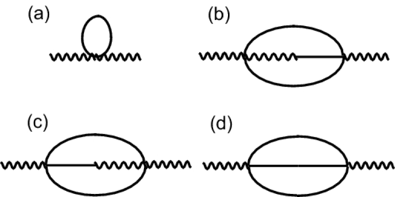
Figure 5: Diagrams that contribute to the noise $D(\omega)$.

Next, we turn to the correlation function $C(t,t^{\prime})=\langle\,x(t)x(t^{\prime})\,\rangle$, which can be written in the form: $C(\omega)=2D(\omega)\left|G(\omega)\right|^{2}$, with $D(\omega)$ are computed from diagrams listed in Fig. 5 and it is given by

$$D(\omega) = D_{0}\left(1+{\gamma T\over k}\right)+k\Gamma_{0}^{2}\gamma^{2}\left[\,3kE(\omega)-8TH(\omega)\,\right]$$

$$E(\omega) = \int{d\omega_{1}\over 2\pi}\,\int{d\omega_{2}\over 2\pi}\,C_{0}(\omega-\omega_{1}-\omega_{2})C_{0}(\omega_{1})C_{0}(\omega_{2}),$$

$$H(\omega) = \int{d\omega_{1}\over 2\pi}\,\int{d\omega_{2}\over 2\pi}\,C_{0}(\omega_{1})C_{0}(\omega_{2})$$

$$\times \left[\,G_{0}(\omega-\omega_{1}-\omega_{2})+G_{0}(\omega_{1}+\omega_{2}-\omega)\,\right].$$

After some algebra, we find

$$D(\omega)=2D_{0}\left[\,1+(\gamma T/k)-6(\gamma T/k)^{2}\,\mbox{Re}\,\mu(\omega/\Gamma_{0}k)\,\right],$$

and we evaluate the correlation function,

$$C(t,0) = {T\over k}\,\left[{3\alpha_{2}-\alpha_{1}\,\left(1+{\gamma T\over k}\right)\over\alpha_{2}^{2}-\alpha_{1}^{2}}\,\right]e^{-\alpha_{1}t}$$ (94)

$$+ {T\over k}\,\left[{\alpha_{2}\,\left(1+{\gamma T\over k}\right)-3\,\alpha_{1}\over\alpha_{2}^{2}-\alpha_{1}^{2}}\,\right]e^{-\alpha_{2}t},$$

with decay rates

$$\alpha_{1} \equiv {\Gamma_{0}k\over 2}\left[\,4+\gamma T/k\,-\sqrt{\,4-4\gamma T/k+25\,(\gamma T/k)^{2}\,}\,\right],$$

$$\approx {\Gamma_{0}k}\left[1+{\gamma T/k}-3\left({\gamma T/k}\right)^{2}\right],\,\,\,\,\mbox{for $\gamma T/k\ll 1$},$$

$$\alpha_{2} \equiv {\Gamma_{0}k\over 2}\left[\,4+\gamma T/k\,+\sqrt{\,4-4\gamma T/k+25\,(\gamma T/k)^{2}\,}\,\right],$$

$$\approx 3\Gamma_{0}k\left[1+(\gamma T/k)^{2}\right],\,\,\,\,\mbox{for $\gamma T/k\ll 1$}.$$

Note that there are now two decaying modes with a fast mode $\alpha_{2}$ and a slow mode $\alpha_{1}$ in the system in contrast to the case with with uniform diffusion. Note also that $\langle x^{2}(0)\rangle=T/k$ as it should be. If we did not put in the extra drift term $gg^{\prime}$ in $f(x)$, this relation would not hold. In fact, it would have been $\langle x^{2}(0)\rangle=T/(k-\gamma T)$, which violates the equipartition theorem. This is yet another demonstration that this extra drift term $gg^{\prime}$ is needed to ensure the correct thermodynamic properties. In Fig. 6, we plot the correlation function in Eq. (94) and the numerical simulation of the Langevin equation describing this system for $\gamma T/k=0.15$. Clearly, the second order perturbation theory agrees very well with the simulation. Note, however, that when $\gamma T/k\sim 1$, $\alpha_{1}$ becomes negative, signalling the breakdown of perturbation theory.

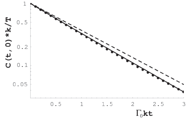
Figure 6: A plot of the correlation function of $x$, $C(t,0)$, as a function of $t$ for $\gamma T/k=0.15$. The solid line represents $C(t,0)$ as given by Eq. (94), which is calculated from the perturbation theory to second order in $\gamma T/k$. The data points are obtained from numerical simulation of the corresponding Langevin equation. Clearly, the result from the perturbation theory agree excellently with the simulation. The dashed line represents the bare (zeroth order) correlation function, which has a decaying rate that is different from the case if the spatial-varying dissipative coefficient.

Finally, we demonstrate FDT to second order in perturbation theory. The physical response function is given by

$$\chi_{xx}(t,t^{\prime}) = \Gamma_{0}\left\langle\,x(t)\,\hat{x}(t^{\prime})\left[\,1+\gamma\,x^{2}(t^{\prime})\,\right]e^{-{\cal S}_{I}}\right\rangle_{0}$$

$$= \Gamma_{0}G(t,t^{\prime})+\Gamma_{0}\gamma G_{0}(t,t^{\prime})C_{0}(0)$$

$$- \Gamma_{0}\gamma\left\langle\,x(t)\,\hat{x}(t^{\prime})x^{2}(t^{\prime}){\cal S}_{I}\right\rangle_{0},$$

which corresponds to the diagrams in Fig. 7. We find

$$\chi_{xx}(\omega)=\Gamma_{0}G(\omega)\left[1+\gamma T/k-6\,(\gamma T/k)^{2}\mu(\omega/\Gamma_{0}k)\right].$$ (95)

Note that this clearly shows that the physical response function and the propagator are different. Taking the imaginary part of Eq. (95), it can be easily verified that the Fluctuation-dissipative theorem Eq. (85) is indeed satisfied to second order in perturbation theory.

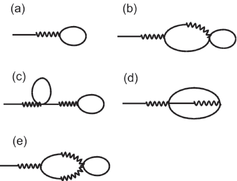
Figure 7: Diagrams that contribute to the physical response function $\chi_{xx}(\omega)$.

V N-Components Langevin Equation

Many physical problems involve more than one variable and some of the issues we have addressed so far may not apply to higher-dimensional systems. For example, the drift term $f(x)$ in 1-D can always be written as a derivative of another function, i.e. 1-D systems are conservative, however, for higher dimensional systems, this may not be true. A complete analysis of higher dimensional systems requires a separate publication. Here, we briefly discuss the Fokker-Planck equation and the path integral in the $\alpha$-convention for a multidimensional Langevin equation of the form

$$\partial_{t}x_{i}=f_{i}(x_{1},\cdots,x_{N})+g_{ij}(x_{1},\cdots,x_{N})\eta_{j}(t),$$ (96)

where $\eta_{i}(t)$ are the noises, with zero mean and correlation given by

$$\langle\,\eta_{i}(t)\eta_{j}(t^{\prime})\,\rangle=\delta_{ij}\delta(t-t^{\prime}).$$ (97)

In Eq. (96) and the following, Einstein summation is assumed. We focus on the case where the system is near thermal equilibrium and address, as we did in the 1D case, how the Boltzmann distribution determines the form of $f_{i}$ and $g_{ij}$ in the $\alpha$-convention. The Fokker-Planck equation corresponds to Eq. (96) can be derived following the same procedure as outlined in Sec. II.3. In the $\alpha$-convention, we find

$${\partial{\cal P}\over\partial t}={\partial\over\partial x_{i}}\left\{-\left[f_{i}+\alpha{\partial g_{il}\over\partial x_{k}}\,g_{kl}\right]\,{\cal P}+{1\over 2}{\partial\over\partial x_{j}}\left(g_{il}\,g_{jl}{\cal P}\right)\right\},$$ (98)

where ${\cal P}[\{x\},t]$ is the joint probability distribution of $x_{i}$ at time $t$. If there are only dissipative terms and no reactive terms in $f_{i}$, the constraint that ${\cal P}$ reach a long-time state of thermal equilibrium value proportional to $\exp-\beta{\cal H}$ requires that

$$f_{i}(\{x\})={1\over 2}{\partial\over\partial x_{j}}\left(g_{ik}\,g_{jk}\right)-\alpha{\partial g_{ij}\over\partial x_{l}}g_{lj}-{1\over 2}\beta g_{ik}g_{jk}{\partial{\cal H}\over\partial x_{j}},$$ (99)

in order that Eq. (98) reduce to

$${\partial{\cal P}\over\partial t}={\partial\over\partial x_{i}}\left({1\over 2}g_{il}\,g_{jl}\right)\left[\beta{\partial{\cal H}\over\partial x_{j}}\,{\cal P}+{\partial{\cal P}\over\partial x_{j}}\right],$$ (100)

with the steady-state solution ${\cal P}\propto\exp-\beta{\cal H}$.

The diffusion matrix is defined as

$$D_{ij}(\{x\})={1\over 2}g_{il}\,g_{jl}=k_{B}T\Gamma_{ij}(\{x\}),$$ (101)

where $\Gamma_{ij}(\{x\})$ is the matrix of dissipative coefficients. Thus

$$f_{i}(\{x\})={\partial D_{ij}(\{x\})\over\partial x_{j}}-\alpha{\partial g_{ij}\over\partial x_{l}}g_{lj}-\Gamma_{ij}(\{x\}){\partial{\cal H}\over\partial x_{j}},$$ (102)

Note that since the diffusion matrix $D_{ij}(\{x\})$ is a symmetric with respect to $i\leftrightarrow j$, it has only $N(N+1)/2$ independent entries, and we may impose $N^{2}-N(N+1)/2=N(N-1)/2$ constraints on $g_{ij}(\{x\})$ without sacrificing the physical content. We could, for example chose $g_{ij}$ to be symmetric in which case, it is simply the square root of $k_{B}T\Gamma_{ij}$

To derive the path integral, we first discretize Eq. (96) as

$$x_{i}^{(n)}=x_{i}^{(n-1)}+\Delta tf_{i}^{(n)}+g_{ij}^{(n)}\int_{t_{n-1}}^{t_{n}}ds\,\eta_{j}(s),$$ (103)

and introduce

$$h_{i}\left[\left\{x_{k}^{(n)}\right\},\left\{x_{k}^{(n-1)}\right\}\right]\equiv[g^{(n)}]_{ij}^{-1}\left[x_{j}^{(n)}-x_{j}^{(n-1)}-\Delta tf_{j}^{(n)}\right]-\int_{t_{n-1}}^{t_{n}}ds\,\eta_{i}(s),$$ (104)

where $f_{i}^{(n)}=f_{i}(\{\alpha x_{i}^{(n)}+(1-\alpha)x_{i}^{(n-1)}\})$ and $g_{ij}^{(n)}=g_{ij}(\{\alpha x_{i}^{(n)}+(1-\alpha)x_{i}^{(n-1)}\})$. Following the basic steps as outlined in Sec. IV, we can write the conditional probability as

$${\cal P}(\{x_{k}^{(n)}\}\,t_{n}|\{x_{k}^{(n-1)}\}\,t_{n-1})=\det\left|{\partial h_{i}\over\,\partial x_{k}^{(n)}}\right|\left\langle\prod_{i=1}^{N}\,\delta\left[h_{i}(\{x_{k}^{(n)}\},\{x_{k}^{(n-1)}\})\right]\right\rangle.$$ (105)

Taking the derivative of $h_{i}$ explicitly, we find

$${\partial h_{i}\over\,\partial x_{k}^{(n)}}=g^{-1}_{il}\left(\,\delta_{lk}-{\cal M}_{lk}\,\right),$$

where we have defined the matrix ${\cal M}_{lk}$ by

$${\cal M}_{lk} \equiv \alpha\Delta t{\partial f_{l}\over\partial x_{k}}+\alpha{\partial g_{lm}\over\partial x_{k}}\,g^{-1}_{ij}\left[\,x_{j}^{(n)}-x_{j}^{(n-1)}-\Delta tf_{j}^{(n)}\right].$$ (106)

Using the identity $\det\hat{X}=\exp\mbox{Tr}\hat{X}$, the determinant can be evaluated to give

$$\det\left|{\partial h_{i}\over\,\partial x_{k}^{(n)}}\right|={1\over\det g_{ij}}\left[\,1-{\cal M}_{ll}+{1\over 2}\,\left({\cal M}_{ll}{\cal M}_{kk}-{\cal M}_{lk}{\cal M}_{kl}\right)+\cdots\right].$$ (107)

Therefore, the conditional probability can be written as

$${\cal P}(\{x_{k}^{(n)}\}\,t_{n}|\{x_{k}^{(n-1)}\}\,t_{n-1})=\prod_{i=1}^{N}\,\int{dk_{i}\over 2\pi\det g_{ij}}\left[1-{\cal M}_{ll}+{1\over 2}\,\left({\cal M}_{ll}{\cal M}_{kk}-{\cal M}_{lk}{\cal M}_{kl}\right)\right]e^{\imath k_{i}g_{ij}^{-1}\left(\Delta x_{j}-\Delta tf_{j}\right)-{1\over 2}k_{i}^{2}\Delta t},$$ (108)

where we have only kept terms up to order $\Delta t$. Following the similar procedure leading to Eq. (53) for the 1-D case, we find

$${\cal P}(\{x_{k}^{(n)}\}\,t_{n}|\{x_{k}^{(n-1)}\}\,t_{n-1}) = \prod_{i=1}^{N}\,\int{dk_{i}\over 2\pi\det g_{ij}}\left[1-\alpha\Delta t\partial_{l}f_{l}+\alpha\imath k_{m}\partial_{l}g_{lm}\Delta t+{\alpha^{2}\over 2}\Delta t\left(\partial_{k}g_{lm}\partial_{l}g_{km}-\partial_{l}g_{lm}\partial_{k}g_{km}\right)\right]$$

$$\times e^{\imath k_{i}g_{ij}^{-1}\left(\Delta x_{j}-\Delta tf_{j}\right)-{1\over 2}k_{i}^{2}\Delta t},$$

$$= \int{dy_{k}\over 2\pi}\,e^{+\imath y_{k}(\Delta x_{k}-f_{k}\Delta t+\alpha\,g_{kj}\partial_{l}g_{lj}\Delta t)-{1\over 2}g_{lk}g_{kj}y_{l}y_{j}-\alpha\Delta t\partial_{l}f_{l}-{\alpha^{2}\over 2}\left(\partial_{k}g_{lm}\partial_{l}g_{km}-\partial_{l}g_{lm}\partial_{k}g_{km}\right)\Delta t},$$

where in the last line, we have exponentiate terms in the bracket and substituted $y_{i}=g_{ij}k_{j}$. In the continuum limit, we have

$${\cal P}(\{x_{k}^{(f)}\}\,t_{f}|\{x_{k}^{(0)}\}\,t_{0})=\int_{x_{k}^{(0)}}^{x_{k}^{(f)}}{\cal D}x_{k}\int{\cal D}y_{k}\,e^{-{\cal S}},$$

$${\cal S}=\int dt\left[{1\over 2}\,g_{lk}g_{jk}y_{l}y_{j}-\imath y_{k}\left(\,\partial_{t}x_{k}-f_{k}+\alpha\,g_{kj}\partial_{l}g_{lj}\,\right)+\alpha\,\partial_{l}f_{l}+{\alpha^{2}\over 2}\,\left(\,\partial_{k}g_{lm}\partial_{l}g_{km}-\partial_{l}g_{lm}\partial_{k}g_{km}\right)\right].$$ (110)

Note that there is an extra term proportional to $\alpha^{2}$. This term is identically zero for 1-D system. If we start with Eq. (V) and follow the procedure as outlined in Sec. IV.1, we can show that the path integral is equivalent to the Fokker-Planck equation in Eq. (98).

VI Conclusion

In this paper, we have examined a thermodynamically consistent Langevin formulation of the Brownian motion with a diffusion coefficient that depends on space. We argue, in particular, that the requirement that the Boltzmann distribution be reached in equilibrium determines the interpretation of stochastic integrals arising from multiplicative noise in the Langevin equation. We hope that this paper clarifies some of the confusion over these stochastic issues that have persisted for some time. We have also constructed path integral representations of the Langevin equations with multiplicative noise, and we used this representation as a starting point for the development of a systematic perturbation theory. Such a formulation can be employed to treat nonlinear stochastic equations arising from a variety of problems. Future work includes generalizing this formulism to “fields” and examines how state-dependent dissipative coefficients may give rise to long-time tails and corrections to scaling in dynamic critical phenomena. Of course, one of the most interesting open questions is whether there is an equivalent criteria for systems that are driven far from equilibrium.

Appendix A Connection between $\alpha$ and $\theta(0)$

In this Appendix, we outline the connection between $\alpha$ and the Heaviside unit step function, $\theta(t)$ evaluated at $t=0$. For simplicity, we set $f(x)=0$ in Eq. (10):

$$\partial_{t}x=g(x)\eta(t).$$ (111)

Using the $\alpha$-convention rule Eq. (8), we have for $\Delta x(t)\equiv x(t+\Delta t)-x(t)$

$$\Delta x(t) = g[x(t)+\alpha\Delta x]\int_{t}^{t+\Delta t}ds\,\eta(s)$$

$$= g[x(t)]\int_{t}^{t+\Delta t}ds\,\eta(s)$$

$$+\,\alpha\,g^{\prime}[x(t)]\,\Delta x(t)\,\int_{t}^{t+\Delta t}ds\,\eta(s)+\cdots$$

$$= g[x(t)]\int_{t}^{t+\Delta t}ds\,\eta(s)$$

$$+\,\alpha gg^{\prime}\int_{t}^{t+\Delta t}ds\,\int_{t}^{t+\Delta t}ds^{\prime}\eta(s)\eta(s^{\prime})+\cdots$$

Therefore, the average $\Delta x(t)$ over the noise is

$$\langle\Delta x(t)\rangle=\alpha gg^{\prime}\int_{t}^{t+\Delta t}ds\,\int_{t}^{t+\Delta t}ds^{\prime}\,\delta(s-s^{\prime}).$$ (112)

The integral

$$\int_{-\infty}^{t}ds^{\prime}\,\delta(s-s^{\prime}) = \left\{\begin{array}[]{cc}0&s>t\\ 1&s<t\end{array}\right.$$ (115)

$$= \theta(t-s),$$ (116)

defines the Heaviside unit step function, $\theta(t)$, and Eq. (112) becomes

$$\langle\Delta x(t)\rangle = \alpha gg^{\prime}\int_{t}^{t+\Delta t}ds\,\left[\theta(t+\Delta t-s)-\theta(t-s)\right]$$ (117)

$$= \alpha\,gg^{\prime}\Delta t.$$

On the other hand, we can directly integrate Eq. (111) to obtain

$$\Delta x(t)=\int_{t}^{t+\Delta t}ds\,g[x(s)]\,\eta(s).$$ (118)

Expanding $g[x(s)]$ as

$$g[x(s)]=g[x(t)+\Delta x(s)]=g[x(t)]+g^{\prime}[x(t)]\Delta x(s)+\cdots,$$ (119)

we find

$$\Delta x(t)=g\int_{t}^{t+\Delta t}\eta(s)+gg^{\prime}\int_{t}^{t+\Delta t}ds\,\int_{t}^{s}ds^{\prime}\eta(s)\eta(s^{\prime}).$$ (120)

Note that the upper limit of integration for $s^{\prime}$ is different from that in Eq. (112). Therefore, we find

$$\langle\Delta x(t)\rangle=\theta(0)\,gg^{\prime}\Delta t.$$ (121)

Comparing this with Eq. (117), we conclude that $\theta(0)=\alpha$.

Appendix B Equivalence between Eq. (49) and Eq. (53)

In this Appendix, we demonstrate that the conditional probability given in Eq. (49) and its exponentiated form, Eq. (53), are indeed equivalent. Note that the latter expression involves a subtle step which is required for the construction of the path integral in Sec. IV. Therefore, it is crucial to confirm Eq. (53) is correct at least to order of $\Delta t$. We have already checked that the correct Fokker-Planck Equation, Eq. (17), can be derived from Eq. (53) in Sec. IV.1. Here, we check that the normalization condition:

$$\int dx_{i}P(x_{i}\,t_{i}|x_{i-1}\,t_{i-1})=1,$$ (122)

for general $\alpha$ is satisfied by Eq. (53). First, let us check Eq. (122) is true for Eq. (49). For simplicity, we set $f(x)=0$. We have

$$\int dx_{i}P(x_{i}t_{i}|x_{i-1}t_{i-1})=\int{d\Delta x_{i}\over\sqrt{2\pi\Delta t}g_{i}}\,e^{-{\Delta t\over 2g_{i}^{2}}\left({\Delta x_{i}\over\Delta t}\right)^{2}}\left[1-\alpha\,{g_{i}^{\prime}\over g_{i}}\,\Delta x_{i}\right]=\int{dw\over\sqrt{2\pi}g_{i}}\left[1-\alpha\,{g_{i}^{\prime}\over g_{i}}\sqrt{\Delta t}\,w\right]e^{-{w^{2}\over 2g_{i}^{2}}}$$ (123)

where we have made a change of variable: $\Delta x_{i}=\sqrt{\Delta t}\,w$. Remembering that $g_{i}=g[x_{i-1}+\alpha\sqrt{\Delta t}\,w]$ and expanding them in Eq. (123) in power of $\Delta t$, we have

$$\int dx_{i}P(x_{i}t_{i}|x_{i-1}t_{i-1})$$

$$=\int{dw\over\sqrt{2\pi}g}e^{-{w^{2}\over 2g^{2}}}\left[1-{2\alpha g^{\prime}\over g}\sqrt{\Delta t}\,w+\left({3\alpha^{2}g^{\prime 2}\over g^{2}}-{3\alpha^{2}g^{\prime\prime}\over 2g}\right)\Delta t\,w^{2}+{\alpha g^{\prime}\over g^{3}}\,\sqrt{\Delta t}\,w^{3}+\left({\alpha^{2}g^{\prime\prime}\over 2g^{3}}-{7\alpha^{2}g^{\prime 2}\over 2g^{4}}\right)\,w^{4}\right.$$

$$\left.\phantom{\left({7\alpha^{2}g^{\prime 2}\over 2g^{2}}\right)}+{\alpha^{2}g^{\prime 2}\over 2g^{6}}\,\Delta t\,w^{6}+\cdots\right]$$ (124)

$$=1+{\cal O}[\Delta t^{3/2}],$$ (125)

where $g\equiv g(x_{i-1})$. Thus, Eq. (49) indeed satisfies the normalization condition, which is hardly surprising since it must be true by construction. Now, let us check the exponentiated from, Eq. (53). We have

$$\int dx_{i}P(x_{i}t_{i}|x_{i-1}t_{i-1})=\int{d\Delta x_{i}\over\sqrt{2\pi\Delta t}g_{i}}\,e^{-{\Delta t\over 2g_{i}^{2}}\left({\Delta x_{i}\over\Delta t}+\alpha g_{i}g_{i}^{\prime}\right)^{2}}=\int{dw\over\sqrt{2\pi}g_{i}}e^{-{\Delta t\over 2g_{i}^{2}}\left({w\over\sqrt{\Delta t}}+\alpha g_{i}g_{i}^{\prime}\right)^{2}},$$

$$=\int{dw\over\sqrt{2\pi}g}e^{-{w^{2}\over 2g^{2}}}\left[1-{1\over 2}\alpha^{2}g^{\prime 2}-{2\alpha g^{\prime}\over g}\sqrt{\Delta t}\,w+\left({7\alpha^{2}g^{\prime 2}\over 2g^{2}}-{3\alpha^{2}g^{\prime\prime}\over 2g}\right)\Delta t\,w^{2}+{\alpha g^{\prime}\over g^{3}}\,\sqrt{\Delta t}\,w^{3}+\left({\alpha^{2}g^{\prime\prime}\over 2g^{3}}-{7\alpha^{2}g^{\prime 2}\over 2g^{4}}\right)\,w^{4}\right.$$

$$\left.\phantom{\left({7\alpha^{2}g^{\prime 2}\over 2g^{2}}\right)}+{\alpha^{2}g^{\prime 2}\over 2g^{6}}\,\Delta t\,w^{6}+\cdots\right]$$ (126)

$$=1+{\cal O}[\Delta t^{3/2}].$$ (127)

Thus, Eq. (53) also satisfies the normalization condition. We note in passing that although the expansions, Eqs. (124) and (126) are different, they both give one at the end result to the lowest order and the next order term is of the order $\Delta t^{3/2}$.

Appendix C alpha-dependent perturbation theory for the model system with $D(x)=D_{0}(1+\gamma x^{2})$

In this Appendix, we carry out a first order perturbation calculation for general $\alpha$ of the model system studied in Sec. IV.3 in which $D(x)=D_{0}(1+\gamma x^{2})$ in order to clarify some subtle issues associated with the $\alpha$-convention. It is straightforward to work out the action in Eq. (57). Up to an irrelevant constant, we have

$${\cal S}_{0} = \int dt\left[-D_{0}\hat{x}^{2}+\hat{x}\left(\partial_{t}x+\Gamma_{0}kx\right)\right]$$

$${\cal S}_{I} = \Gamma_{0}\gamma\int dt\left[2(2\alpha-1)x\hat{x}+{k\over T}\,x^{3}\hat{x}-\,x^{2}\hat{x}^{2}\right.$$

$$- \left.3\,\alpha\,{k\over T}\,x^{2}\right].$$

Note that there are more diagrams to evaluate than there are for $\alpha=0$. Consider first the propagator $G(t,t^{\prime})=\langle x(t)\hat{x}(t^{\prime})\rangle$, which can be written as $G^{-1}(\omega)=G_{0}^{-1}(\omega)+\Sigma(\omega)$, where the diagrams for the self-energy are displayed in Fig. 8. Note that the closed loop diagram c in Fig. 8 contains $G_{0}(t=0)$ which must be set to $\alpha$ as explained in Sec. IV.2. We find

$$\Sigma(\omega) = 2(2\alpha-1)D_{0}\gamma+3D_{0}\gamma-4D_{0}\gamma G_{0}(0)$$

$$= D_{0}\gamma,$$

which agrees with the calculation for $\alpha=0$. Note that the final result is independent of $\alpha$ as it should be. To first order, the noise $D(\omega)$ renormalizes exactly the same way as in the $\alpha=0$ calculation. However, the physical response function is different. It is given by Eq. (IV.2) with an extra $\alpha$ dependent term:

$$\chi_{xx}(t,t^{\prime}) = \Gamma_{0}\left\langle\,x(t)\,\hat{x}(t^{\prime})\left[\,1+\gamma\,x^{2}(t^{\prime})\,\right]e^{-{\cal S}_{I}}\right\rangle_{0}$$

$$- {\alpha\over T}\left\langle\,x(t)[2\,\gamma D_{0}x(t^{\prime})]e^{-{\cal S}_{I}}\right\rangle_{0}$$

$$= \Gamma_{0}\left(1+{\gamma T\over k}\right)G(t,t^{\prime})+2\alpha\Gamma_{0}\gamma C_{0}(t,t^{\prime})$$

$$- 2\alpha\Gamma_{0}\gamma C_{0}(t,t^{\prime})+{\cal O}(\gamma^{2})$$

. $$= \Gamma_{0}\left(1+{\gamma T\over k}\right)G(t,t^{\prime}).$$

Without the cancellation of the $\alpha$ dependent terms, $\chi_{xx}(t,t^{\prime})$ would not have been causal.

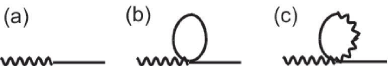
Figure 8: Diagrams that contribute to the self-energy $\Sigma(\omega)$.

References

- (1) For a recent review, see E. Frey and K. Kroy, Ann. Phys.(Leipzig) 14, 20 (2005).
- (2) N.G. van Kampen, Stochastic Processes in Physics and Chemistry. (North-Holland, Amsterdam 1992).
- (3) H. Risken, The Fokker-Planck Equation. (Springer-Verlag, NY, 1989).
- (4) C.W. Gardiner, Handbook of Stochastic Methods for Physics, Chemistry and the Natural Sciences. (Springer-Verlag, NY, 1983).
- (5) J. Zinn-Justin, Quantum Field Theory and Critical Phenonmena, 4th ed. (Oxford University Press, NY, 2003).
- (6) L.F. Cugliandolo, in Slow relaxations and nonequilibrium dynamics in condensed matter, (Springer, NY, 2003).
- (7) J.D. Murray, Mathematical Biology, 3rd ed. (Springer Verlag, Heidelberg, 2002).
- (8) P.M. Chaikin and T.C. Lubensky, Principles of Condensed Matter Physics (Cambridge University Press, New York, 1995).
- (9) J. Howard, Mechanics of Motor Proteins and the Cytoskeleton, (Sinauer Associates, 2001).
- (10) D.C. Morse, Advances in Chem. Phys. 128, 65 (2004).
- (11) P. Lancon, G. Batrouni, L. Lobry, and N. Ostrowsky, Europhys. Lett. 54, 28 (2001); Physica A 304, 65 (2002).
- (12) J.C. Neto, R. Dickman, O.N. Mesquita, Physica A 345, 173 (2005); E. Goshen, W.Z. Zhao, G. Carmon, S. Rosen, R. Granek, M. Feingold, Phys. Rev. E, 71, 061920 (2005).
- (13) V. Blickle, T. Speck, L. Helden, U. Seifert, and C. Bechinger, Phys. Rev. Lett. 96, 070603 (2006).
- (14) J.-C. Meiners and S.R. Quake, Phys. Rev. Lett. 82, 2211 (1999); S. Henderson, S. Mitchell, and P. Bartlett, Phys. Rev. E 64, 061403 (2001).
- (15) T. Bickel and R. Bruinsma, Biophys. J. 83, 3079 (2002).
- (16) W. Cai and T.C. Lubensky, Phys. Rev. E 52, 4251 (1995).
- (17) J.C. Crocker and D.G. Grier, Phys. Rev. Lett. 73, 352 (1994); J. Colloid Interface Sci. 179, 298 (1996).
- (18) D.L. Ermak and J.A. McCammon, J. Chem. Phys. 69, 15 (1978).
- (19) J.M. Sancho, M. San Miguel, and D. Dürr, J. Stat. Phys. 28, 291 (1982).
- (20) M. Doi and S.F. Edwards, The Theory of Polymer Dynamics (Clarendon Press, Oxford, 1994).
- (21) N.G. van Kampen, J. Stat. Phys. 24, 175 (1981).
- (22) P. Arnold, Phys. Rev. E 61, 6091 (2000); Phys. Rev. E 61, 6099 (2000).
- (23) B. Øksendal, Stochastic Differential Equations. (Springer, NY, 2000).
- (24) M.J. Schnitzer, Phys. Rev. E 48, 2553 (1993).
- (25) J.C. Crocker, J. Chem. Phys. 106, 2837 (1997).
- (26) R. Verma, J.C. Crocker, T.C. Lubensky, and A.G. Yodh, Macromolecules 33, 177 (2000).
- (27) M.P. Lettinga, E. Barry, and Z. Dogic, Europhys. Lett. 71, 692 (2005).
- (28) H. Brenner, Chem. Eng. Sci. 16, 242 (1961).
-
(29)
For all numerical simulations done in this paper, we employ the
Miltstein scheme:
where is a time step, and is a Gaussian distributed random variable with zero mean and variance of . See, for example, P.E. Kloeden and E. Platen, Numerical Solution of Stochastic Differential Equations. (Springer, NY, 1995). - (30) L.P. Faucheux and A.J. Libchaber, Phys. Rev. E 49, 5158 (1994).
- (31) E.R. Dufresne, D. Altman, and D.G. Grier, Europhys. Lett. 53, 264 (2001).
- (32) P.C. Martin, E.D. Siggia, H.A. Rose, Phys. Rev. A 8, 423 (1973).
- (33) R. Phythian, J. Phys. A: Math. Gen. 10, 777 (1977); B. Jouvet and R. Phythian, Phys. Rev. A 19, 1350 (1979).
- (34) R. Graham, in Springer Tracts in Modern Physics in Solid State, Vol. 66 (Springer-Verlag, NY, 1973).
- (35) H.K. Janssen, Z. Phys. B 23, 377 (1976).
- (36) K. Miyazaki and D.R. Reichman, J. Phys. A: Math. Gen. 38, L343-L355 (2005).