Saturation model in the non-Glauber approach

Abstract:

In this paper a new saturation model is presented. This model is based on the theoretical solution for the generating functional, and it is quite different and not more complicated than the Glauber-like approach used before. The model describes the structure function $F_{2}$ of the proton, as well as the diffractive structure function $F_{2}^{D}$. We show the difference between our model and the eikonal approach by calculating the multiplicity distribution, using the AGK cutting rules strategy.

1 Introduction

The very intriguing observation of the HERA experiments is the rapid rise of the total $\gamma^{*}p$ cross section, with energy in the deep inelastic scattering (DIS) region. The linear evolution equations approach is not valid in the region of high energies, since it predicts an increase of the parton density, steeper than is allowed by the Froissart bound. The solution to this problem is hidden in the effect of the parton saturation. At high energy the density of partons increases, filling the whole transverse area of the target. This stage is called saturation. At small values of Bjorken-$x$, the interaction between partons should be taken into account leading to the recombination of partons. This process tames the growth of the parton density.

The main goal of this paper is to build a model which follows on from the self consistent theoretical approach, and is able to describe the matching between soft and hard processes. This approach is based on the generating functional method. The model incorporates the following features :

$\;\;\;i$) Evolution of the parton density with energy

$\;ii$) The phenomena of parton saturation. The model takes into account the effect of parton recombination at high density and preserves unitarity.

$\;iii$) This is a simple model, different from the model based on the eikonal approach.

$\;iv$) Good description of all recent experimental data on inclusive, hard, soft, and diffractive processes.

In the next section, we start with a brief discussion of the main properties of the generating functional [1]. We find the solution to the simplified evolution equation, assuming that the dipoles do not change their transverse sizes, during the interaction.

Based on this solution, we build our model. All details and properties of the model are discussed in section 2. This model is quite different from the other saturation models, which are based on the eikonal approach [2, 3, 4, 5, 6, 7]. In section 3, we show how our model describes the HERA data using the recent data on the proton structure function $F_{2}$, in a wide range of kinematics from different collaborations [8, 9, 10, 11, 12, 13, 15, 14, 16], we fit our model and find the free parameters. We compare the developed model, to other saturation models in section 4, where we discuss the multiplicity distribution of the two models, and we present the differences between them. In the next section using the parameters from the fit, we describe the diffractive dissociation experimental data, the charm quark structure function $F^{c\overline{c}}_{2}$, and the slopes $dF_{2}/d(\ln Q^{2})$ and $d\ln F_{2}/d(\ln 1/x)$. Finally, we summarize our results.

2 Description of the Model

2.1 General properties of the generating functional

This approach is based on the concept of color dipoles [1], which in the large $N_{c}$ limit are correct degrees of freedom at high energies [17], since they diagonalize the scattering matrix. At high energy, every parton tends to emit more partons, which leads to the evolution of the initial parton density. The dipole decay produces a parton cascade, originating from the one parent dipole at initial high rapidity $Y$. We define by $P_{n}$ to be the probability to obtain $n$ dipoles from the parent dipole, at some rapidity $y$.

Using the generating functional approach, one can construct an evolution equation for the dipole probability $P_{n}$ at rapidity $y$ [18]. The interesting property of this approach, is the manifestation of the saturation phenomena, and the conservation of unitarity. For the sake of simplicity, we consider the generating functional approach in the toy-model [18, 19], where we neglect changes to the dipole sizes during interaction. In this approach, we obtain the following evolution equation for the probability $P_{n}$

$$-\frac{\partial P_{n}}{\partial y}\,=\,-\omega_{0}nP_{n}\,+\,\omega_{0}(n-1)P_{n-1}$$ (2.1)

where $\omega_{0}$ is the probability for one dipole to decay into two. The generating functional, with our assumption degenerates into the function

$$Z(y,\,u)\,\,=\,\,\sum_{n}\,\,P_{n}(y)\,\,u^{n}\,,$$ (2.2)

Equation Eq. (2.1), for the probability $P_{n}$ can be rewritten in terms of the generating functional Eq. (2.2), as

$$-\,\,\frac{\partial\,Z(y,\,u)}{\partial\,y}\,\,=\,\,-\,\omega_{0}\,u\,(1\,-\,u)\,\,\frac{\partial\,Z(y,\,u)}{\partial\,u}$$ (2.3)

This is a Liouville equation which has the solution

$$Z(y_{0}-y,\,u)\,\,=\,\,\frac{u\,\,e^{\,-\,\omega_{0}\,(y-y_{0})}}{1\,\,+\,\,u\,\,(e^{\,-\,\omega_{0}\,(y\,-\,y_{0})}\,-\,1)}\,.$$ (2.4)

To find the interaction amplitude, we follow the procedure suggested in Ref.[20], namely,

$$N(y,\,b)\,\,=\,\,Im\,A^{el}(y,\,b)\,\,=\,\,-\sum^{\infty}_{n=1}\,\,\frac{1}{n!}\,\,\frac{\partial^{n}Z}{(\partial u)^{n}}|_{u=1}\,\,\gamma_{n}(b)\,\,=\,\,-\sum^{\infty}_{n=1}\,\,\frac{1}{n!}\,\,\frac{\partial^{n}Z}{(\partial u)^{n}}|_{u=1}\,\,\gamma^{n}_{1}(b)$$ (2.5)

Here, $-\,\gamma_{n}(b)$ is the imaginary part of the amplitude for the scattering of $n$ dipoles off the target, at fixed impact parameter $b$, at low energies. The most important assumption, is the independent interaction of $n$ dipoles with the target, which is expressed by the factor $\gamma_{n}=\gamma^{n}_{1}$ factor in Eq. (2.5).

2.2 The Model

Using the generating functional approach, we propose a model for the interaction amplitude of the dipole with the target. The amplitude $N(y,\,b)$ can be found from the following relation

$$N(y;\,b,\,r)\,\,=\,\,1\,\,-\,\,Z(y,\,u(r))\,.$$ (2.6)

Inserting Eq. (2.4) into Eq. (2.6), one obtains the final expression for the interaction amplitude

$$N(y;\,b,\,r)\,=\,\frac{(1-u)e^{\omega_{0}(y-y_{0})}}{(1-u)e^{\omega_{0}(y-y_{0})}\,+\,u}\,=\,\frac{\gamma(r)e^{\omega_{0}(y-y_{0})}}{\gamma(r)e^{\omega_{0}(y-y_{0})}\,+\,(1-\gamma(r))}$$ (2.7)

Eq. (2.7) describes the sum of so-called”fan” diagrams. Introducing the new variable [21]

$$\gamma_{R}\;=\;\frac{\gamma}{1-\gamma}$$ (2.8)

the amplitude now has the simple form

$$N(y;\,b,\,r)\,=\,\frac{\gamma_{R}(y_{0};\,b,\,r)e^{\omega_{0}(y-y_{0})}}{\gamma_{R}(y_{0};\,b,\,r)e^{\omega_{0}(y-y_{0})}\,+\,1}$$ (2.9)

and satisfies the following equation

$$\frac{\partial N(y;\,b,\,r)}{\partial y}\;=\;\omega_{0}\gamma_{R}\,\frac{\partial N(y;\,b,\,r)}{\partial\gamma_{R}}$$ (2.10)

This means that in fact, the generating functional describes the system of non-interacting hard pomerons, but its interaction with the target should be renormilized using Eq.(2.8). Our main assumption, is that we can include the dependence on the size of the dipoles incorporates it in the low energy amplitude $\gamma$ condition.

$$\gamma_{R}(y_{0};\,b)\;\rightarrow\;\gamma_{R}(y_{0};\,b,\,r)$$ (2.11)

where $r$ is the transverse size of the dipole. At small values of $r$, the amplitude of Eq. (2.9) should match the expression originating from the perturbative calculation of the BFKL pomeron exchange, namely

$$\Omega\,=\,\gamma_{R}(y_{0};\,b,\,r)e^{\omega_{0}(y-y_{0})}\;\equiv\;\frac{\pi^{2}}{N_{c}}r^{2}\alpha_{s}(\mu^{2})G(y_{0},\mu^{2})G(y-y_{0},\mu^{2})S(b)$$ (2.12)

where $G(y-y_{0},\mu^{2})$ is the gluon density at some scale $\mu^{2}$, $y$ is the rapidity defined in Eq. (2.12) as $y\;=\;\ln(1/x)$, and S(b) stands for the proton profile function in the form

$$S(b)\,=\,\frac{2}{\pi R^{2}}\left(\frac{\sqrt{8}b}{R}\right)K_{1}\left(\frac{\sqrt{8}b}{R}\right)$$ (2.13)

where $K_{1}$ is the McDonald function. The evolution of the parton density is given by the DGLAP evolution equation, with the initial parton density at some scale $Q^{2}_{0}$

$$G(x,Q^{2}_{0})\,=\,\frac{A}{x^{\omega_{0}}}$$ (2.14)

where $A$ and $\omega_{0}$ are to be determined from the data fit. The expression for the gluon density $G(x,Q^{2})$, is obtained from the solution to the DGLAP equation, and is given by the inverse Mellin transform [22]

$$G(y,t)=\frac{1}{2\pi i}\int_{c-i\infty}^{c+i\infty}d\omega\exp(\frac{t}{\omega}-t+\omega y)\frac{A}{(\omega-\omega_{0})}$$ (2.15)

where the variable $t$ is defined as

$$t=\frac{4N_{c}}{b_{0}}\ln\frac{\ln(Q^{2}/\Lambda^{2})}{\ln(Q_{0}^{2}/\Lambda^{2})},\,\,\,\ b_{0}=(11-\frac{2n_{f}}{3}),\;\;\;\mbox{and}\,\,\,y\,=\,\ln(1/x)$$ (2.16)

where $Q^{2}_{0}$ is the initial condition, and $n_{f}$ is the number of flavors. The analytical solution to Eq. (2.15) reads as

$$G(y,t)\,=\,Ae^{-t+\omega_{0}y}\left[\int_{0}^{y}dy^{{}^{\prime}}e^{-\omega_{0}y^{{}^{\prime}}}\sqrt{\frac{t}{y^{{}^{\prime}}}}I_{1}(2\sqrt{ty^{\prime}})\,+\,1\right]$$ (2.17)

Here, we introduce the hard scale $\mu^{2}$, which corresponds to the transverse size of the dipoles in the following way

$$Q^{2}\rightarrow\mu^{2}\,=\,\frac{C}{r^{2}}\,+\,\mu^{2}_{0}$$ (2.18)

where we rewrite the gluon density in terms of $\mu^{2}$, rather than $Q^{2}$. The parameters $C$ and $\mu^{2}_{0}$, are obtained from the fit to data. Finally, the expression for the interaction amplitude takes the following form

$$N(r,b,x)\,=\,\frac{\Omega(r,b,x)}{\Omega(r,b,x)+1}$$ (2.19)

with

$$\Omega(r,b,x)\;=\;\frac{\pi^{2}}{N_{c}}\,r^{2}\,\alpha_{s}\left(\mu^{2}(r)\,\right)G\left(\ln(1/x_{0}),\mu^{2}(r)\right)\,G\left(\ln(x/x_{0}),\mu^{2}(r)\right)\,S(b)$$ (2.20)

This is a new form for the interaction amplitude of the dipoles with the target, which originates from the generating functional approach.

2.3 Saturation Scale

At some energy value, partons start to populate densely, and this leads to the effect of saturation. We define a new scale, which separates the two regions, namely, the region of low parton density, where we can apply perturbative methods, and the region of high parton density, where we should take into account the recombination effects, and non-liner corrections to the parton density. In order to determine the saturation scale, we demand that the packing factor of the partons Eq. (2.21), at some energy, be equal to 1. The packing factor is defined as

$$\kappa\;=\;\sigma_{0}\frac{N_{g}}{\pi R^{2}}$$ (2.21)

where $\sigma_{0}$ is the typical interaction cross section of the partons, which is proportional to $Q^{2}$. $N_{g}$ corresponds to the number of partons, and $\pi\,R^{2}$ denotes the area of the transverse slice of the hadron. Putting everything together, one obtains

$$1\, = \,\frac{\pi^{2}}{N_{c}}r^{2}_{s}\alpha_{s}(\mu_{s}^{2})G(y_{0},\mu_{s}^{2})G(y-y_{0},\mu_{s}^{2})S(b)$$

$$1\, = \,\frac{4}{Q^{2}}\frac{\pi^{2}}{N_{c}}\alpha_{s}(\mu_{s}^{2})G(y_{0},\mu_{s}^{2})G(y-y_{0},\mu_{s}^{2})S(b)$$

$$Q^{2}_{s}(x)\, = \,4\frac{\pi^{2}}{N_{c}}\alpha_{s}(\mu_{s}^{2})G(y_{0},\mu_{s}^{2})G(y-y_{0},\mu_{s}^{2})S(b)$$ (2.22)

where $\mu^{2}_{s}\,=\,\frac{CQ^{2}_{s}}{4}\,+\,\mu^{2}_{0}$. The estimation of the saturation momentum is obtained from the numerical solution of the Eq. (2.3) by iteration. The result obtained for the saturation scale is plotted in Fig. 2.1.

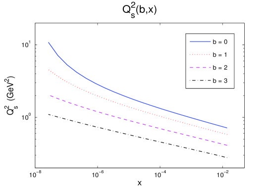
Figure 2.1: Saturation scale for various values of impact parameter b(fm) as a function of Bjorken-x.

Different graphs correspond to different values of the impact parameter $b$. The value of the saturation scale, is calculated in units of $GeV^{2}$.

3 Description of DIS

We start by overviewing the main features of DIS. The deep inelastic scattering process is shown in Fig. 3.1$(a)$

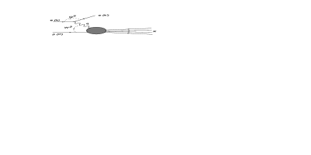
(a)	(b)

Figure 3.1: Kinematics of deep inelastic scattering and photon-gluon fusion diagram.

and the standard variables are defined as

incoming proton momentum $$: \;\;\;P$$

photon’s virtuality $$: \;\;\;Q^{2}=-q^{2}$$

fraction of electron energy transferred to the proton $$: \;\;\;y\,=\,\frac{P\cdot q}{P\cdot k}$$

photon - proton system energy $$: \;\;\;(q+P)^{2}\,=\,W^{2}$$

Bjorken-$$x : \;\;\;x=\frac{Q^{2}}{2p\cdot q}\,=\,\frac{Q^{2}}{Q^{2}+W^{2}}$$

For small values of Bjorken-$x$, one can separate between the photon wave function, which corresponds to the creation of the quark - antiquark pair, and the interaction of the dipole with the target [23, 24]. In the dipole picture of DIS, the total photon-proton scattering cross section from transverse (T) and longitudinal (L) polarized virtual photons, is given by the convolution of the photon wave function, $\Psi_{T,L}$, and the interaction amplitude $N$ of the dipoles with the target Eq. (2.19). The proton structure function $F_{2}$, can be written as the sum of two contributions [24]

$$F_{2}(x,Q^{2})\,=\,2\sum_{n=1}^{n_{f}}\frac{Q^{2}}{4\pi^{2}\alpha_{em}}\int d^{2}r\int d^{2}b\int_{0}^{1}dz\left\{|\Psi_{T}(r,z;m_{f},e_{f})|^{2}\,+\,|\Psi_{L}(r,z;m_{f},e_{f})|^{2}\right\}N(r,b,x)$$ (3.2)

where $f$ stands for the flavor of the quark-antiquark pair, and $m_{f}$ and $e_{f}$, denote the mass and electric charge of the quark with flavor $f$, respectively. The squared wave function of the photon is given by

$$|\Psi_{T}(r,z;m_{f},e_{f})|^{2}\,=\,\frac{N_{c}e_{f}^{2}\alpha_{em}}{2\pi^{2}}\left\{[z^{2}+(1-z)^{2}]a^{2}K_{1}^{2}(ar)+m_{f}^{2}K_{0}^{2}(ar)\right\}$$ (3.3)

and

$$|\Psi_{L}(r,z;m_{f},e_{f})|^{2}\,=\,\frac{N_{c}e_{f}^{2}\alpha_{em}}{2\pi^{2}}\left\{4Q^{2}z^{2}(1-z)^{2}K_{0}^{2}(ar)\right\}$$ (3.4)

where

$$a^{2}\,=\,z(1-z)Q^{2}+m^{2}_{f}$$ (3.5)

and $K_{1}$, $K_{0}$ where $K_{1}$, $K_{0}$ are McDonald functions. The significant contribution to the inclusive processes, appears from the heavy quark production. In the present paper we investigate the influence of the charm quark contribution to the proton structure function $F_{2}$.

3.1 Heavy quark

The recent data from HERA, shows that the heavy quark contribution is up to 30%-40% of the total value of the structure function [11, 12], and can not be neglected. Thus, we take into account the contribution of the charm quark and confront it with recent data. The analysis does not include any new parameters. The proton structure function may be written, as the contribution from all possible participating quarks. Since the contribution of each quark flavor is proportional to its electromagnetic charge, and to the inverse mass, we may conclude that the contribution of very heavy quarks like, top and bottom, can be neglected compared with the light quarks (i.e. up, down, strange) and also the charm quark. The light quark masses are considered to be the same. Hence, the proton structure function may be written as

$$F_{2}\;=\;F_{2}^{u\overline{u}}\;+\;F_{2}^{d\overline{d}}\;+\;F_{2}^{s\overline{s}}\;+\;F_{2}^{c\overline{c}}$$ (3.6)

Each component of the structure function associated with different quark flavors, is proportional to the particular quark wavefunction of the corresponding flavor,

$$F_{2}^{f\overline{f}}(x,Q^{2})\,=\,2\frac{Q^{2}}{4\pi\alpha_{em}}\int d^{2}b\int d^{2}r\int dz|\Psi^{f\overline{f}}(r,z;m_{f},e_{f})|^{2}N(r,b,x^{f\overline{f}})$$ (3.7)

In the case of the charm quark, its contribution to the total structure function, has the following form

$$F_{2}^{c\overline{c}}(x,Q^{2})\,=\,2\frac{Q^{2}}{4\pi\alpha_{em}}\int d^{2}b\int d^{2}r\int dz|\Psi^{c\overline{c}}(r,z;m_{c},e_{c})|^{2}N(r,b,x^{c\overline{c}})$$ (3.8)

where the photon wavefunction, which decays into the charm-anticharm pair is given by

$$|\Psi^{c\overline{c}}(r,z;m_{c},e_{c})|^{2}\,=\,\frac{N_{c}\alpha_{em}}{2\pi^{2}}\frac{4}{9}\{[z^{2} + (1+z)^{2}]a^{2}K_{1}^{2}(ar)+m^{2}_{c}K_{0}^{2}(ar)$$ (3.9)

$$+ 4Q^{2}z^{2}(1-z)^{2}K_{0}^{2}(ar)\}$$

where $a^{2}$ is given by Eq. (3.5), and the numerical factor $\frac{4}{9}$ is the squared value of the charge quantum number of the charm, in units of $e$. It is important to stress, that every quark flavor has an independent value of Bjorken-$x$, which depends on the quark mass. This point is presented in the next section.

3.2 Redefinition of Bjorken $x$

The important ingredient of our approach, is the redefinition of Bjorken-$x$. The motivation for this comes from the saturated region, or the region which lies below the saturation scale ($Q^{2}<Q^{2}_{s}$). In this region, the transverse momentum of the partons is proportional to the saturation scale, and this leads to the new definition of Bjorken-$x$

$$4m^{2}\, = \,(q\,+\,k)^{2}$$

$$4m^{2}\, = \,-Q^{2}+2P\cdot q+k^{2}\,=\,-Q^{2}+2P\cdot q-Q^{2}_{s}$$

$$\widetilde{x}\, = \,\frac{Q^{2}\,+\,Q^{2}_{s}\,+\,4m^{2}}{Q^{2}\,+W^{2}}$$ (3.10)

The kinematics is shown in Fig. 3.1$(b)$ We can easily see, that this new definition of Bjorken-$x$ allows a smooth transition from large values of $Q^{2}$, to the region of low values of $Q^{2}$. At large $Q^{2}$, we get back the ordinary expression for Bjorken-$x$, and at low values of photon virtuality, the main contribution comes from the saturation scale.

3.3 Description of Fit

From the fit to the experimental data, we can find values of the appropriate parameters for our model. For this purpose, we use all the latest data for the proton structure function $F_{2}$ from different collaborations in the region $x<0.01$ and $0.045<Q^{2}<150\,\,GeV^{2}$. The small $x$ cut leads to an upper limit on $Q^{2}$ [8, 9, 10, 11, 12, 13, 14, 15, 16]. It was observed, that the set of data from [8] should be rescaled with the factor of $1.037$, in order to satisfy the best fit. For the numerical evaluation, we have implemented the formulae Eqs. (3.2) - (3.4). We have also included the contribution from the heavy charm quark Eq. (3.8), and the new definition of Bjorken-$x$ Eq. (3.2). The model contains free parameters, whose values are to be determined from the fit to the experimental data. The result of our fit, with four quark flavors is represented in table 1.

	$A$	$\mu^{2}_{0}$	$\omega_{0}$	$Q^{2}_{0}$	$C$	$m_{q}$	$m_{c}$	$\chi^{2}/d.o.f.$
four quarks (u,d,s,c)	0.785	1.294	0.060	1.236	1.0	0.24	1.3	354/341

Table 1: The parameters determined from the fit to the proton structure function $F_{2}$

The parameters have the following physical meaning. $A$ with $\omega_{0}$ and $C$ with $\mu^{2}_{0}$ and $Q^{2}_{0}$, determine the hard scale and the initial gluon density, respectively. We observed, that the parameter $C$, has a strong correlation to other parameters. For every value of $C$, it is possible to find a set of four parameters, which satisfy almost the same $\chi^{2}$. Hence, it was fixed with the arbitrary value $C\,=1.0$. The value of the light quark mass, which corresponds to the best fit is $m_{q}\,=\,0.24\,\,(GeV)$. For the charm quark, the mass was taken to be $m_{c}\,=\,1.3\,\,(GeV)$. The reson for taking the same values for the three light quarks ($u,d,s$) originates from the fact, that the influence of the strange quark to the total fit is relatively small, since its contribution in comparison with $u$ and $d$ is proportional to the ratio of charges squared. The resulting fit is plotted in Figs. 3.2, 3.3.

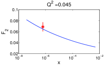
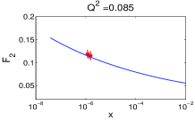
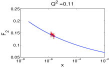
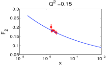
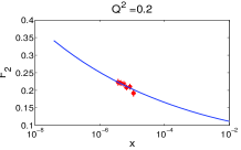
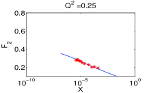
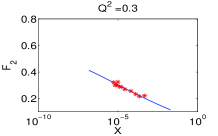
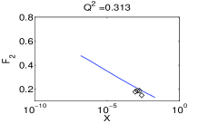
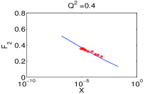
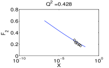
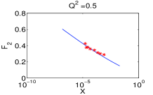
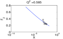
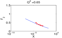
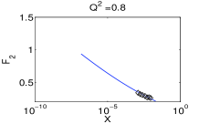
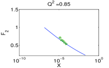
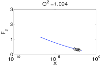
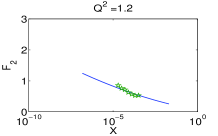
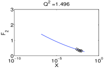
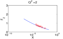
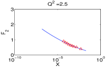
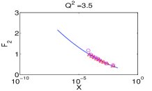
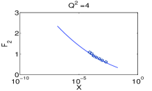
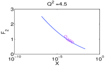
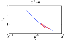
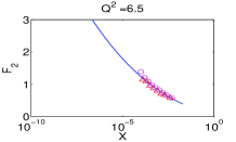
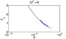
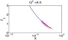
Figure 3.2: $F_{2}(x,Q^{2})$ structure function of proton, as a function of Bjorken $x$ for fixed value of photon virtuality $Q^{2}$. This data was taken for small values of $x<0.01$. These data points correspond to different collaborations. Asterisk corresponds to [10], diamond to [15] collaboration, pentagram to [13], triangles [8], circles correspond to [9] and hexagons to [14].

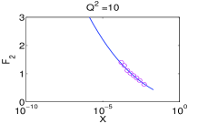
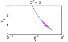
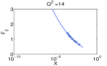
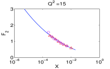
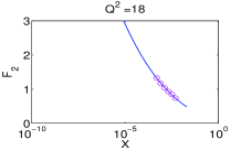
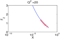
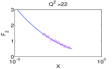
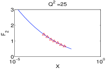
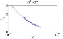
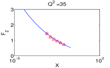
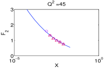
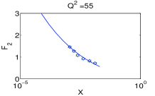
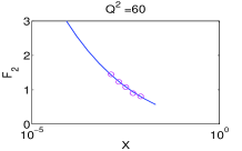
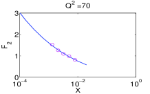
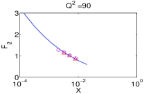
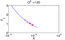
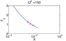
Figure 3.3: (continued) $F_{2}(x,Q^{2})$ structure function of proton, as a function of Bjorken $x$ for fixed value of photon virtuality $Q^{2}$. This data was taken for small values of $x<0.01$ These data points correspond to different collaborations. Asterisk corresponds to [10], triangles [8], circles correspond to [9] and hexagons to [14].

4 Analysis of the model

4.1 Comparison between the models

The most widely spread saturation model, is based on the eikonal approach and has the following form

$$\frac{d\sigma}{d^{2}b}\,\equiv\,N(r,b,x)\,=\,2\left(1\,-\,e^{-\frac{\Omega(r,b,x)}{2}}\right)$$ (4.1)

where $\Omega$ is defined in Eq. (2.12). Using the AGK cutting rules [25], we can calculate the cross sections with different multiplicities $k$. This is the content of the AGK rules, and which relates the cross-section $\sigma_{k}$ for observing a final state with $k$-cut Pomerons, with the amplitudes for the exchange of $m$ Pomerons $F^{(m)}$

$$\frac{d\sigma_{k}}{d^{2}b}\,=\,\sum_{m=k}^{\infty}(-1)^{m-k}2^{m}\frac{m!}{k!(m-k)!}F^{(m)}$$ (4.2)

We will apply this concept and calculate the predictions for the $k$-cut cross-sections. We make a comparison between two models

$$N^{I}\,=\,2\frac{\Omega}{\Omega+1}\;\;\;\;\;\mbox{and}\;\;\;\;\;N^{I\!\!I}\,=\,2\left(1-e^{-\frac{\Omega}{2}}\right)$$ (4.3)

For small values of $\Omega$, the dipole cross sections in Eq. (4.3) are equal to $\Omega$, and are proportional to the gluon density. This allows one to identify the opacity, with the single Pomeron exchange amplitude of Fig. 4.1.

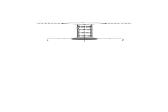
Figure 4.1: The single gluon-ladder contribution to the total $\gamma^{*}$ P cross section

Hence, the multiple Pomeron amplitude is determined from the expansion of the amplitudes in the form of a series expansion. For our model we obtain

$$N^{I}\,=\,2\sum^{\infty}_{m=1}(-1)^{m-1}\Omega^{m}$$ (4.4)

with

$$F^{(m)}_{I}\,=\,\Omega^{m}$$ (4.5)

and for the eikonal model, the same procedure leads to

$$N^{I\!\!I}\,=\,2\sum^{\infty}_{m=1}(-1)^{m-1}\left(\frac{\Omega}{2}\right)^{m}\frac{1}{m!}$$ (4.6)

where

$$F^{(m)}_{I\!\!I}\,=\,\left(\frac{\Omega}{2}\right)^{m}\frac{1}{m!}$$ (4.7)

The dipole cross section can be rewritten [26] in terms of $F^{(m)}$, as a sum over multi-Pomeron amplitudes

$$N\,=\,2\sum_{m=1}^{\infty}(-1)^{m-1}F^{(m)}$$ (4.8)

The expression for the $k$ cut Pomeron cross section, is obtained from the AGK cutting rules of Eqs.(4.2), (4.5) and (4.7)

$$\frac{d\sigma_{k}^{I}}{d^{2}b}\, = \,\sum^{\infty}_{m=k}(-1)^{m-k}\,2^{m}\frac{m!}{k!(m-k)!}\,\Omega^{m}\,=\,\frac{1}{1+2\Omega}\left(\frac{2\Omega}{1+2\Omega}\right)^{k}$$ (4.9)

and

$$\frac{d\sigma_{k}^{I\!\!I}}{d^{2}b}\, = \,\sum^{\infty}_{m=k}(-1)^{m-k}\,2^{m}\frac{m!}{k!(m-k)!}\left(\frac{\Omega}{2}\right)^{m}\frac{1}{m!}\,=\,\frac{\Omega^{k}}{k!}e^{-\Omega}$$ (4.10)

The diffractive cross-section, is given by the difference between the total, and the sum over all cut cross sections

$$\frac{d\sigma_{diff}}{d^{2}b}\,=\,\frac{d\sigma_{tot}}{d^{2}b}\,-\,\sum_{k=1}^{\infty}\frac{d\sigma_{k}}{d^{2}b}$$ (4.11)

and for two models reads as follows

$$\frac{d\sigma_{diff}^{I}}{d^{2}b}\,=\,2\left(\frac{\Omega}{1+\Omega}\right)\,-\,\frac{2\Omega}{1+\Omega}\,=\,\frac{2\Omega^{2}}{(2\Omega+1)(\Omega+1)}$$ (4.12)

and

$$\frac{d\sigma_{diff}^{I\!\!I}}{d^{2}b}\,=\,2\left(1-e^{-\frac{\Omega}{2}}\right)\,-\,(1-e^{-\Omega})\,=\,\left(1-e^{-\frac{\Omega}{2}}\right)^{2}$$ (4.13)

Since we want to compare to different-valued functions, we need to normalize them. Finally, we compare between the ratios

$$R_{k}^{I}\;=\;\frac{d\sigma_{k}^{I}/d^{2}b}{d\sigma_{el}^{I}/d^{2}b}$$ (4.14)

and

$$R_{k}^{I\!\!I}\;=\;\frac{d\sigma_{k}^{I\!\!I}/d^{2}b}{d\sigma_{el}^{I\!I}/d^{2}b}$$ (4.15)

where

$$\frac{d\sigma_{el}}{d^{2}b}\;=\;\sum_{k=1}^{\infty}\frac{d\sigma_{k}}{d^{2}b}$$ (4.16)

Below we present the plots describing the partial normalized cross sections $(d\sigma_{k}/d^{2}b)/(d\sigma_{el}/d^{2}b)$, which correspond to $k$-cut Pomerons and the diffractive cross section $(d\sigma_{diff}/d^{2}b)$. We compare the two models. Our approach, uses a solution of the non-linear evolution equation in a ”toy-model” approach, and the Glauber approach. Our plots were calculated for fixed values of the dipole size $r=0.1fm$, and the value $x_{b}\;=\;0.001$. Since higher cuts ($k>1$) are strongly suppressed, they were rescaled by a factor $10^{3k}$.

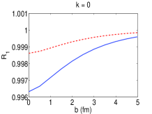
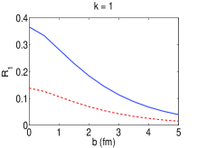
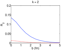
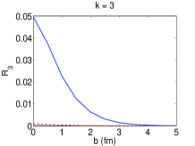
Figure 4.2: Cross sections with different multiplicities as a function of impact parameter $b\;(fm)$. Solid line corresponds to our model and dashed line to the eikonal approach.

Although both models fit the DIS data quite well, there is a difference in the value, and in the shape of the partial cross sections, as shown in the plots.

4.2 Shadowing corrections

In this subsection, we want to discus the difference in the behavior of the two models (our model and the Glauber-like model), from the shadowing corrections point of view. Shadowing corrections (SC), are defined as the next to leading order terms in the series expansion of the amplitude near the amplitude zero point.

$$N^{GF}\; = \;\frac{\Omega_{Gf}}{\Omega_{Gf}+1}\;=\;\Omega_{Gf}-\Omega_{Gf}^{2}+\Omega_{Gf}^{3}-...$$ (4.17a)

$$N^{Gl}\; = \;1-e^{-\frac{\Omega_{Gl}}{2}}\;=\;\frac{\Omega_{Gl}}{2}-\frac{\Omega_{Gl}^{2}}{4\cdot 2!}+\frac{\Omega_{Gl}^{2}}{8\cdot 3!}-...$$ (4.17b)

We can easily conclude, that our proposed generating functional $(GF)$ based model, and the Glauber-like $(Gl)$ function, are the same at leading order, as was expected. Assuming this, we immediately obtain the next condition

$$\Omega_{Gl}\;=\;2\Omega_{Gf}$$ (4.18)

Since we want to check the difference in the behavior of the two different parameterizations, we substitute the condition of Eq. (4.18) into Eq. (4.17b). Finally, we obtain, the fact that our model, predicts larger SC than those proposed by the Glauber-like model.

$$SC^{GF}\;\equiv\;N^{GF}-\Omega_{Gf}\;=-\Omega_{Gf}^{2}+\Omega_{Gf}^{3}-...$$ (4.19a)

$$SC^{Gl}\;\equiv\;N^{Gl}-\Omega_{Gl}\;=-\frac{\Omega_{Gf}^{2}}{2!}+\frac{\Omega_{Gf}^{2}}{3!}-...$$ (4.19b)

It is obvious that $SC^{GF}>SC^{Gl}$. In spite of the fact that, generically, the $SC^{GF}$ are larger, we can fit all the experimental data, using the Glauber parametrization. It turns out that $\Omega_{Gl}$, in such a parametrization, is larger than $\Omega_{Gf}$ by $20-30\%$. The leading term is significant in the low energy domain, and should be consistent with the perturbative calculations of the amplitude. SC becomes significant at higher energies, especially in the saturation domain. Our model predicts the slower growth of the amplitude with energy, than that of the Glauber model.

5 Predictions and descriptions within our model

5.1 Charm quark contribution

The developed dipole model, allows us to calculate a prediction for the inclusive charm quark contribution, to $F_{2}$ of the proton. Using the ansatz Eq. (3.8), we can easily obtain the contribution to the structure function from the charm quark $F_{2}^{c\overline{c}}$.

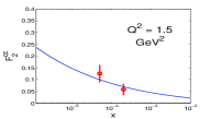
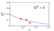
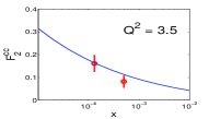
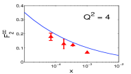
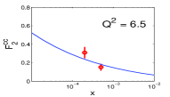
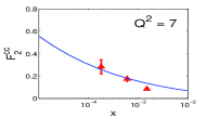
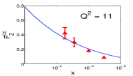
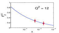
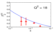
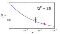
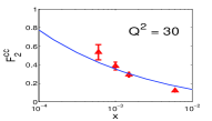
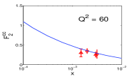
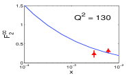
Figure 5.1: Prediction of our model to $F^{c\overline{c}}_{2}$. Solid line is our model, triangles correspond to H1 96-97 and circles to ZEUS 99-00 data [12, 11] respectively. Mass of the charm quark has the value: $m_{c}\;=\;1.3\;\;GeV^{2}$

Comparing this to the recent experimental data [12, 11] we find a good agreement between the calculated prediction, and the experimental result, as it can be viewed in Fig. 5.1.

5.2 Description of $\partial F_{2}/\partial(\ln Q^{2})$ in HERA and the LHC kinematic region

In this section, we want to check how our model is able to describe the slope of the structure function, as a function of the photon virtuality $Q^{2}$, for fixed values of Bjorken-$x$, and vice versa. For this purpose, we calculate the logarithmic derivative of $F_{2}$

$$\lambda_{Q^{2}}\;\equiv\;\frac{\partial F_{2}}{\partial(\ln Q^{2})}$$ (5.1)

Since the only dependence on the virtuality $Q^{2}$, is in the photon wavefunction, the resulting expression for the calculation has the following form

$$\frac{\partial F_{2}}{\partial(\ln Q^{2})}\;=\;Q^{2}\frac{\partial F_{2}}{\partial Q^{2}}\;=\;Q^{2}\frac{\partial}{\partial Q^{2}}\left(\frac{Q^{2}}{4\pi^{2}\alpha}\sigma(x,Q^{2})\right)\;=\;F_{2}\;+\;\frac{Q^{4}}{4\pi^{2}\alpha}\frac{\partial\sigma(x,Q^{2})}{\partial Q^{2}}$$ (5.2)

and

$$\frac{\partial\sigma(x,Q^{2})}{\partial Q^{2}}\;=\;2\int_{0}^{\infty}d^{2}b\int_{0}^{\infty}d^{2}r\int_{0}^{1}dz\;\frac{\partial|\Psi(r,z,Q^{2})|^{2}}{\partial Q^{2}}\,N(r,x,b)$$ (5.3)

where $|\Psi(r,z,Q^{2})|^{2}$ and $N(r,x,b)$ are defined in Eq. (3.4) and Eq. (2.19), respectively. The resulting plots are presented in Figs. 5.2, 5.3 for fixed values of $Q^{2}$ and $x$ respectively. Note, that these sets of experimental data, were not take into account in the fitting procedure.

$\partial F_{2}/\partial(\ln Q^{2})$

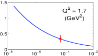
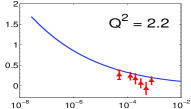
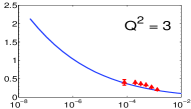
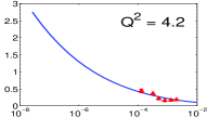
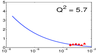
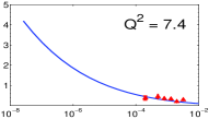
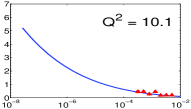
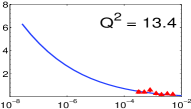
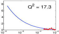
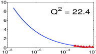
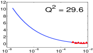
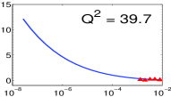
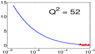
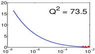
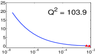
x

Figure 5.2: Prediction of our model to logarithmic derivative $\partial F_{2}/\partial(\ln Q^{2})$ as a function of Bjorken-$x$ for fixed values of $Q^{2}$.

$\partial F_{2}/\partial(\ln Q^{2})$

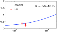
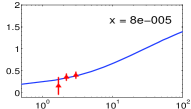
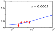
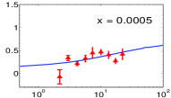
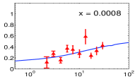
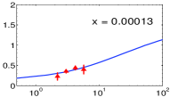
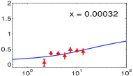
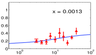
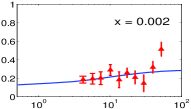
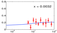
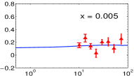
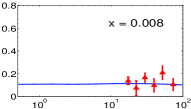
$Q^{2}$  $(GeV^{2})$

Figure 5.3: Logarithmic derivative of $F_{2}$ as a function of $Q^{2}$ for fixed values of Bjorken-$x$. Solid line is our model and triangles correspond to H1 96-97 [8] respectively.

We can see, that predictions which are based on our model, fits well with all experimental data on logarithmic derivative of $F_{2}$. We enlarged the kinematic region towards very low $x$ values, to give predictions for $\lambda_{Q^{2}}$ in the HERA and the LHC kinematic region.

5.3 Description of $\partial\ln F_{2}/\partial(\ln 1/x)$

In this subsection, we present our computation of $\lambda_{x}\;\equiv\;\partial\ln F_{2}/\partial(\ln 1/x)$. A comparison of our prediction with the H1 experimental data [16] is shown in Figs. 5.4, 5.5 for a fixed value of $Q^{2}$ and Bjorken-$x$ respectively.

$\partial\ln F_{2}/\partial(\ln\;1/x)$

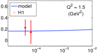
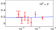
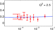
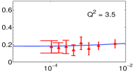
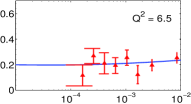
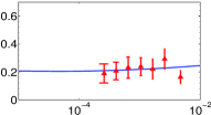
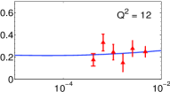
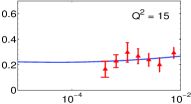
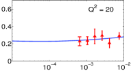
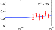
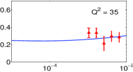
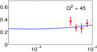
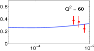
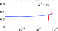
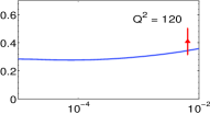
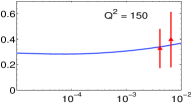
x

Figure 5.4: The logarithmic derivative $\lambda_{x}\;=\;\partial\ln F_{2}/\partial(\ln\;1/x)$ as a function $x$ for fixed values of photon virtuality $Q^{2}$. Data taken from [16].

$\partial\ln F_{2}/\partial(\ln\;1/x)$

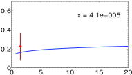
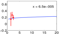
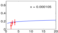
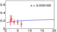
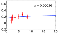
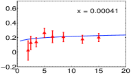
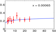
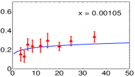
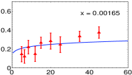
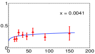
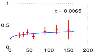
$Q^{2}$

Figure 5.5: The logarithmic derivative $\lambda_{x}$ as a function of $Q^{2}$ for fixed values of Bjorken-$x$.

We can see a good agrement with the experimental data. In order to investigate the behavior of the slope $\lambda_{x}$, in the high energy limit (very low $x$ and $Q^{2}$), we expand our predictions to this region. The result is plotted in Fig. 5.6. We want to pointed out the fact, that our model predicts a behavior of the structure function at the region of small photon virtualities $Q^{2}<1\;GeV^{2}$ which is in good agreement with that obtained by Donnachie and Landshoff [27] from the fit to data.

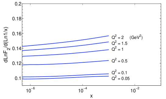
Figure 5.6: The prediction for logarithmic derivative $\lambda_{x}\;=\;\partial\ln F_{2}/\partial(\ln\;1/x)$ plotted at very low $x$ and $Q^{2}$.

5.4 Prediction for $F_{L}$ at HERA

Here, we want to present our predictions for the longitudinal part of the $F_{2}$ structure function $F_{L}$. This longitudinal part, originates from the scattering of the longitudinally polarized virtual photon, off the proton target. The expression for the calculation has the following form

$$F_{L}(x,Q^{2})\;=\;\frac{Q^{2}}{4\pi^{2}\alpha}2\int d^{2}b\int d^{2}r\int dz|\Psi_{L}(r,z,Q^{2})|^{2}N(r,b,x)$$ (5.4)

where $|\Psi_{L}(r,z,Q^{2})|^{2}$ corresponds to the longitudinal part of the photon wavefunction squared Eq. (3.4), and $N(r,b,x)$ is the interaction amplitude Eq. (2.19). We used the relevant data on $F_{L}$ from H1 collaboration [8] in order to estimate our calculations. The experimental values of the longitudinal structure function, are not measured, rather they are extracted from the total structure function $F_{2}$. The extraction of the longitudinal structure function, is based on the reduced cross section Eq. (5.5), which depends on two proton structure functions, $F_{2}(x,Q^{2})$ and $F_{L}(x,Q2)$

$$\sigma_{r}\;\equiv\;F_{2}(x,Q^{2})\;-\;\frac{y^{2}}{1+(1+y)^{2}}F_{L}(x,Q2)$$ (5.5)

where is $y$ defined in Eq. (3). From the reconstruction of the kinematical variable, the desired data on $F_{L}$ were obtained. Our main idea, is to predict the behavior of the longitudinal part of the structure function, in the HERA kinematic region ($x<10^{-5}$), and to check how it fits the existing extracted data. The resulting plots are presented in Fig. 5.7

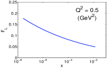
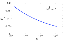
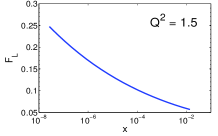
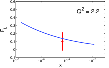
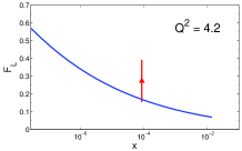
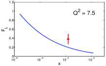
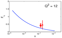
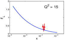
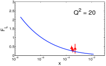
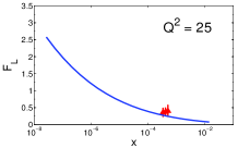
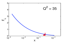
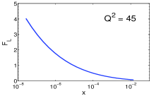
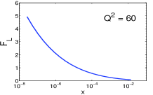
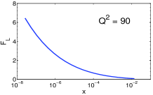
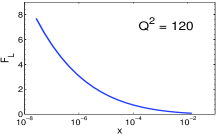
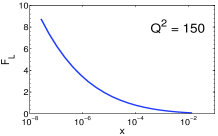
Figure 5.7: Prediction for the $F_{L}$ structure function at the HERA kinematics. The values of $Q^{2}$ are given in $GeV^{2}$.

5.5 Diffractive production in DIS

Diffractive deep inelastic scattering is usually characterized by two variables, the mass of the diffractive system $M^{2}_{X}$, and the momentum transfer $t\,=\,(P-P^{{}^{\prime}})^{2}$. These variables are usually rewritten in terms of other, dimensionless variables as

$$x_{I\!\!P}\,=\,\frac{Q^{2}+M^{2}-t}{Q^{2}+W^{2}}$$ (5.6)

which is the fractional energy-loss suffered by the incident proton and

$$\beta\,=\,\frac{Q^{2}}{Q^{2}+M^{2}-t}$$ (5.7)

which corresponds to the momentum fraction, carried by a struck parton. The pomeron, which carries longitudinal momentum $x_{I\!\!P}$, is emitted by the proton, and subsequently undergoes hard scattering satisfying

$$x_{B}\,=\,x_{I\!\!P}\beta$$ (5.8)

The diffractive dissociation process is depicted in Fig. 5.8

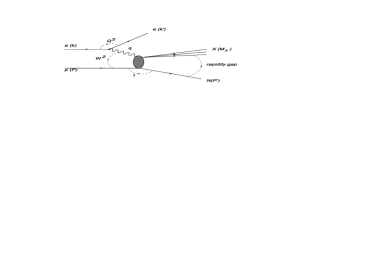
Figure 5.8: Kinematic variables of semi-inclusive reaction $ep\rightarrow eNX$ diffractive dissociation

The important property of the wavefunction formalism, is the ability to describe the diffractive scattering processes [28]. At small values of the diffractive mass $M^{2}$, the elastic scattering of the $q\overline{q}$ pair, dominates, and the corresponding diffractive structure function reads as

$$F^{D}_{2}(x,Q^{2})_{T,L}\,=\,\frac{Q^{2}}{4\pi^{2}\alpha_{em}}\sum_{f=1}^{n_{f}}\int d^{2}b\int d^{2}r\int_{0}^{1}dz|\Psi_{T,L}(r,z;m_{f},e_{f})|^{2}N^{2}(r,b,x)$$ (5.9)

However, at larger values of the mass $M^{2}$, the $q\overline{q}g$ contribution dominates, due to gluon production in the final diffractive state. We take into account the three leading twist terms

$$F^{D(3)}_{2}\,=\,F_{q\overline{q}}^{T}+F_{q\overline{q}}^{L}+F_{q\overline{q}g}^{T}$$ (5.10)

We introduce the last term in Eq. (5.10), to describe high mass diffraction, and as a simple approximation of the first ”fan” diagram, in which the emission of large numbers of gluons is taken into account. The longitudinal part $F_{q\overline{q}g}^{L}$, has no leading logarithm in $Q^{2}$, and can be neglected. The Feynman diagram for the interaction of a quark-antiquark dipole, with the target proton via two-gluon exchange, is shown in Fig.5.9. The gluons couple to the quark in all possible ways.

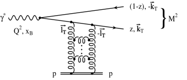
Figure 5.9: $q\overline{q}$ contribution to diffractive DIS, where $z$ represents the fraction of the energy of the photon that is carried by a quark. $M$ is an invariant mass of diffractive system

We follow the procedure proposed in Ref. [29, 3] and we obtain

$$F^{L}_{q\overline{q}}(x_{I\!\!P},\beta,Q^{2})\, = \,\frac{3Q^{4}}{\pi^{3}x_{I\!\!P}(1-\beta)}\int_{0}^{\infty}\,d^{2}b\,\int^{\frac{1}{4}M^{2}-m^{2}}_{0}\frac{dk^{2}_{\perp}}{\sqrt{1-4\frac{m^{2}_{\perp}}{M^{2}}}}\left(\frac{m^{2}_{\perp}}{M^{2}}\right)^{3}\phi^{2}_{0}(k,b,\beta,x_{I\!\!P})$$ (5.11)

and the transverse $q\overline{q}$ contribution has the form

$$F^{T}_{q\overline{q}}(x_{I\!\!P},\beta,Q^{2})\, = \,\frac{3Q^{2}}{x_{I\!\!P}4\pi^{2}}\sum_{f}e^{2}_{f}\int_{0}^{\infty}\,d^{2}b\,\int^{\frac{1}{4}M^{2}-m^{2}}_{0}\frac{dk^{2}_{\perp}}{\sqrt{1-4\frac{m^{2}_{\perp}}{M^{2}}}}\left(\frac{m_{\perp}^{2}}{M^{2}}\right)\times$$ (5.12)

$$\left\{\left(1-\frac{2m^{2}_{\perp}}{M^{2}}\right)\left(\frac{\beta k^{2}+m^{2}_{f}}{1-\beta}\right)\phi^{2}_{1}(k,b,\beta,x_{I\!\!P})\,+\,m^{2}_{f}\,\phi^{2}_{0}(k,b,\beta,x_{I\!\!P})\right\}$$

where

$$M^{2}\,=\,\frac{Q^{2}(1-\beta)}{\beta}\;\;\;\;\mbox{with}\;\;\;\;m^{2}_{\perp}\,=\,k^{2}_{\perp}\,+\,m^{2}_{f}$$ (5.13)

and the ”impact factor” $\phi_{i}(k,b,\beta,x_{I\!\!P})$ $(i=0,1,2)$ given by:

$$\phi_{i}(k,b,\beta,x_{I\!\!P})\,=\,\int\,dr\,r\,K_{i}\left(\sqrt{\frac{k^{2}_{\perp}\beta+m^{2}_{f}}{1-\beta}}r\right)J_{i}(kr)N(x_{I\!\!P},r,b)$$ (5.14)

where $K_{i}$ and $J_{i}$ are Bessel functions. This impact factor, represents the interaction between the produced dipole from the virtual photon, and the target.

The next contribution $q\overline{q}g$, was calculated assuming the strong ordering in the transverse momenta of the gluon and the $q\overline{q}$ dipole, namely $k_{\perp g}\ll k_{\perp q,\overline{q}}$. This assumption allows us to treat the $q\overline{q}$, and $q\overline{q}g$, as an effective color dipole in the transverse $r$ space. The corresponding diagram is plotted in Fig. 5.10.

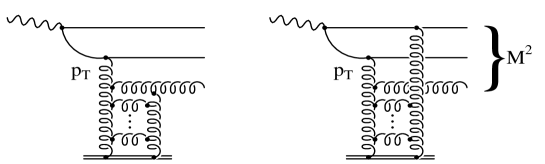
Figure 5.10: $q\overline{q}g$ contribution with strong ordering with the gluon. Gluon’s transverse momentum is considered to be smaller than the (anti)quark’s one.

Thus, we obtain:

$$F_{q\overline{q}g}^{T}(\beta,Q^{2},x_{I\!\!P})\,=\,\frac{81\beta}{16\pi^{2}x_{I\!\!P}}\sum_{f}e^{2}\frac{\alpha_{s}(Q^{2})}{2\pi}\int^{1}_{\beta}\frac{d\beta^{{}^{\prime}}}{\beta^{{}^{\prime}}}\left[\left(1-\frac{\beta}{\beta^{{}^{\prime}}}\right)^{2}\,+\,\left(\frac{\beta}{\beta^{{}^{\prime}}}\right)^{2}\right]$$

$$\times\,\frac{\beta^{{}^{\prime}}}{(1-\beta^{{}^{\prime}})^{3}}\int_{0}^{\infty}\,d^{2}b\,\int^{Q^{2}(1-\beta^{{}^{\prime}})}_{0}dk^{2}_{\perp}\,\ln\left(\frac{Q^{2}(1-\beta^{{}^{\prime}})}{m^{2}_{\perp}}\right)\,\phi^{2}_{2}(k,b,\beta^{{}^{\prime}},x_{I\!\!P})$$ (5.15)

Using the developed model (see section 2.2), which successfully fitted all the experimental data on DIS, we want to describe diffractive DIS, using the same model and parameters which were obtained from the fit. For this purpose, we used the latest data on diffractive dissociation, from ZEUS collaboration [14]. The resulting plots, are shown in Figs. 5.11, 5.12.

$M_{X}=1.2\,GeV$	$M_{X}=3\,GeV$	$M_{X}=6\,GeV$	$M_{X}=11\,GeV$	$M_{X}=20\,GeV$	$M_{X}=30\,GeV$
$Q^{2}=2.7\,GeV^{2}$
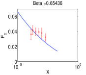
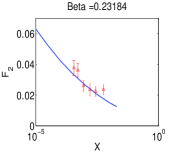
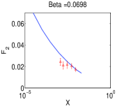
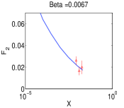
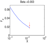
$4\,GeV^{2}$
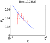
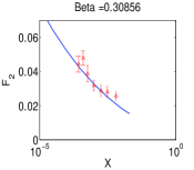
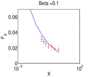
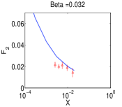
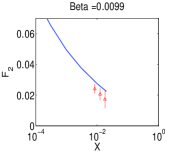
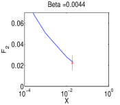
$6\,GeV^{2}$
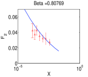
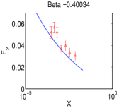
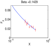
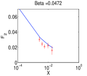
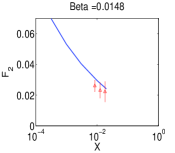
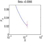
$8\,GeV^{2}$

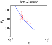
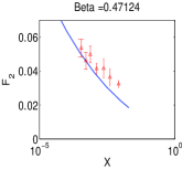
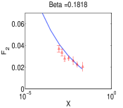
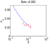
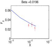
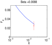
Figure 5.11: Diffractive dissociation structure function $F_{2}^{D(3)}(\beta,x_{I\!\!P},Q^{2})$ as a function of $x_{I\!\!P}$. Comparison of the prediction of the model with ZEUS data [14].

$M_{X}=1.2\,GeV$	$M_{X}=3\,GeV$	$M_{X}=6\,GeV$	$M_{X}=11\,GeV$	$M_{X}=20\,GeV$	$M_{X}=30\,GeV$
$14\,GeV^{2}$
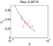
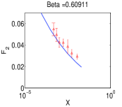
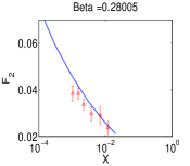
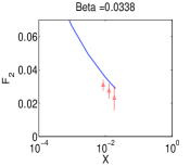
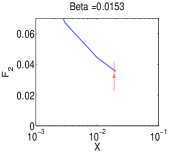
$27\,GeV^{2}$
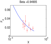
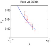
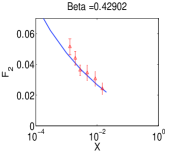
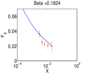
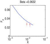
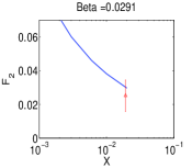
$55\,GeV^{2}$

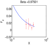
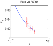
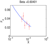
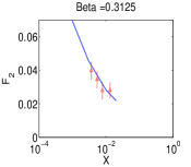
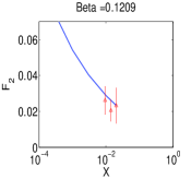
Figure 5.12: (continued) Diffractive dissociation structure function $F_{2}^{D(3)}(\beta,x_{I\!\!P},Q^{2})$ as a function of $x_{I\!\!P}$. Comparison of the prediction of the model with ZEUS data [14].

6 Summary

Using the generating functional approach, we develop a new saturation model, which describes well all the HERA data on deep inelastic scattering and diffractive dissociation. We took into account the QCD evolution, by evolving the initial gluon density with the DGLAP evolution equation. The innovation used in this current work, is the redefinition of Bjorken-$x$, in the saturation region, since the transverse momentum of partons cannot be neglected, and it is the saturation scale. We included in the calculation of the proton structure function $F_{2}$, the contribution from heavy quark production, and also investigated the behavior of the $F_{2}^{c\overline{c}}$ structure function. The resulting $\chi^{2}/d.o.f$ for the fit of DIS data, is very close to one ($\chi^{2}/d.o.f\;=\;354/341$) and this reflects the fact that our new model is able to give reliable predictions. This was justified in the case of the description of diffractive dissociation data, using the same parameters which were obtained from the fit to DIS. Despite the fact that two completely different models are able to describe well the experimental data, we can distinguish between them by calculating the differential cross sections with various multiplicities $d\sigma^{k}/d^{2}b$. From figures shown, we can easily see the different behavior of these cross sections, as a function of the impact parameter $b$. From the plot of the saturation scale 2.1, we can conclude, that up to the scale $\thicksim\;$3 - 4 $GeV^{2}$, saturation is significant, and the non-linear interaction term in the evolution equation, plays an essential role. We believe that this paper, introduces an additional argument for the saturation phenomenon. It shows that the saturation models are able to describe all experimental data, including small values of $Q^{2}$ and low $x$. The description does not depend on the model assumptions widely used instead of the solution to the equation in the mean field approximation [30], which turns out to be rather complicated.

7 Acknowledgments

I would like to express my deep appreciation to Eugene Levin for his support in writing this paper. I am also very grateful to Asher Gotsman, Alex Prygarin, Jeremy Miller, and Alex Palatnik for fruitful discussions on the subject. Special thanks to Erez Etzion, Gideon Bella, Jonatan Ginzburg, Nir Amram and Eran Naftali for the technical support and essential discussions on the experimental background of the research. This research was supported in part by the Israel Science Foundation, founded by the Israeli Academy of Science and Humanities and by BSF grant # 20004019.

References

- [1] A. H. Mueller, Nucl. Phys. B 415, 373 (1994).
- [2] K. Golec-Biernat and M. Wusthoff, Phys. Rev. D 59 (1999) 014017 [arXiv:hep-ph/9807513].
- [3] K. Golec-Biernat and M. Wusthoff, Eur. Phys. J. C 20 (2001) 313 [arXiv:hep-ph/0102093].
- [4] J. Bartels, K. Golec-Biernat and H. Kowalski, Phys. Rev. D 66 (2002) 014001 [arXiv:hep-ph/0203258].
- [5] H. Kowalski and D. Teaney, Phys. Rev. D 68 (2003) 114005 [arXiv:hep-ph/0304189].
- [6] K. Golec-Biernat and S. Sapeta, Phys. Rev. D 74 (2006) 054032 [arXiv:hep-ph/0607276].
- [7] H. Kowalski, L. Motyka and G. Watt, Phys. Rev. D 74 (2006) 074016 [arXiv:hep-ph/0606272].
- [8] C. Adloff et al. [H1 Collaboration], Eur. Phys. J. C 21, 33 (2001) [arXiv:hep-ex/0012053].
- [9] S. Chekanov et al. [ZEUS Collaboration], Eur. Phys. J. C 21 (2001) 443 [arXiv:hep-ex/0105090].
- [10] J. Breitweg et al. [ZEUS Collaboration], Phys. Lett. B 487 (2000) 53 [arXiv:hep-ex/0005018].
- [11] S. Chekanov et al. [ZEUS Collaboration], Phys. Rev. D 69 (2004) 012004 [arXiv:hep-ex/0308068].
- [12] C. Adloff et al. [H1 Collaboration], Phys. Lett. B 528 (2002) 199 [arXiv:hep-ex/0108039].
- [13] C. Adloff et al. [H1 Collaboration], Nucl. Phys. B 497 (1997) 3 [arXiv:hep-ex/9703012].
- [14] S. Chekanov et al. [ZEUS Collaboration], Nucl. Phys. B 713 (2005) 3 [arXiv:hep-ex/0501060].
- [15] M. R. Adams et al. [E665 Collaboration], Phys. Rev. D 54 (1996) 3006.
- [16] C. Adloff et al. [H1 Collaboration], Phys. Lett. B 520 (2001) 183 [arXiv:hep-ex/0108035].
- [17] A. H. Mueller, Nucl. Phys. B 415 (1994) 373; ibid B 437 (1995) 107. E. Levin, Phys. Rev. D 49, 4469 (1994).
- [18] E. Levin and M. Lublinsky, Nucl. Phys. A 730 (2004) 191 [arXiv:hep-ph/0308279]. E. Levin and M. Lublinsky, Phys. Rev. Lett. B 607 131 (2005) arXiv:hep-ph/0411121.
- [19] A. H. Mueller, Nucl. Phys. B 437 (1995) 107.
- [20] Yu. Kovchegov, Phys. Rev. D 60 (2000) 034008.
- [21] E. Levin and A. Prygarin, arXiv:hep-ph/0701178.
- [22] R. K. Ellis, Z. Kunszt and E. M. Levin, Nucl. Phys. B 420 (1994) 517 [Erratum-ibid. B 433 (1995) 498].
- [23] A. H. Mueller, Nucl. Phys. B 335 (1990) 115.
-
[24]
J.R. Forshaw and D.A. Ross, QCD and the Pomeron, Cambridge
University Press, 1997;
N. Nikolaev and B. G. Zakharov, Z. Phys. C 53 (1992) 331;
V. Barone, M. Genovese, N. N. Nikolaev, E. Predazzi and B. G. Zakharov, Phys. Lett. B 326 (1994) 161 [arXiv:hep-ph/9307248]. - [25] V. A. Abramovsky, V. N. Gribov and O. V. Kancheli, Yad. Fiz. 18 (1973) 595 [Sov. J. Nucl. Phys. 18 (1974) 308].
- [26] A. H. Mueller and G. P. Salam, Nucl. Phys. B 475 (1996) 293 [arXiv:hep-ph/9605302].
- [27] A. Donnachie and P. V. Landshoff, Nucl. Phys. B 244 (1984) 322.
- [28] N. Nikolaev and B. G. Zakharov, Z. Phys. C 53 (1992) 331.
- [29] E. M. Levin, A. D. Martin, M. G. Ryskin and T. Teubner, Z. Phys. C 74 (1997) 671 [arXiv:hep-ph/9606443].
-
[30]
M. Lublinsky, Eur. Phys. J. C 21 (2001)
513 [arXiv:hep-ph/0106112];
E. Levin and M. Lublinsky, Nucl. Phys. A 712 (2002) 95 [arXiv:hep-ph/0207374];
N. Armesto and M. A. Braun, Eur. Phys. J. C 20 (2001) 517 [arXiv:hep-ph/0104038];
K. J. Golec-Biernat, L. Motyka and A. M. Stasto, Phys. Rev. D 65 (2002) 074037 [arXiv:hep-ph/0110325];
E. Gotsman, E. Levin, M. Lublinsky and U. Maor, Eur. Phys. J C 27 (2003) 411 [arXiv:hep-ph/0209074];
E. Gotsman, M. Kozlov, E. Levin, U. Maor and E. Naftali, Nucl. Phys. A 742 (2004) 55 [arXiv:hep-ph/0401021];
E. Iancu, A. H. Mueller and S. Munier, Phys. Lett. B 606 (2005) 342 [arXiv:hep-ph/0410018];