Observational constraints on the braneworld model
with brane-bulk energy exchange

Abstract

We investigate the viability of the braneworld model with energy exchange between the brane and bulk, by using the most recent observational data related to the background evolution. We show that this energy exchange behaves like a source of dark energy and can alter the profile of the cosmic expansion. The new Supernova Type Ia (SNIa) Gold sample, Supernova Legacy Survey (SNLS) data, the position of the acoustic peak at the last scattering surface from the Wilkinson Microwave Anisotropy Probe (WMAP) observations and the baryon acoustic oscillation peak found in the Sloan Digital Sky Survey (SDSS) are used to constrain the free parameters of this model. To infer its consistency with the age of the Universe, we compare the age of old cosmological objects with what computed using the best fit values for the model parameters. At $68\%$ level of confidence, the combination of Gold sample SNIa, Cosmic Microwave Background (CMB) shift parameter and SDSS databases provide $\Omega_{m}=0.29_{-0.02}^{+0.03}$, $\Omega_{A}=-0.71_{-0.03}^{+0.03}$ and $\mu=-0.40_{-0.26}^{+0.28}$, hence a spatially flat Universe with $\Omega_{K}=0.00_{-0.04}^{+0.04}$. The same combination with SNLS supernova observation give $\Omega_{m}=0.27_{-0.02}^{+0.02}$, $\Omega_{A}=-0.74_{-0.02}^{+0.04}$ and $\mu=0.00_{-0.30}^{+0.30}$ consequently provides a spatially flat Universe $\Omega_{K}=-0.01_{-0.03}^{+0.04}$. These results obviously seem to be compatible with the most recent WMAP results indicating a flat Universe.

1 Introduction

Recent observations of type Ia supernovas (SNIa) suggest the expansion of the Universe is accelerating (A.G. Riess el. al., 1998; S. Perlmutter et al., 1999; A. G. Riess el. al., 2004; J. L. Tonry el. al., 2003). As it is well known all usual types of matter with positive pressure generate attractive forces, which decelerate the expansion of the Universe. A “dark energy” component with negative pressure was suggested to account for the invisible fuel that drives the current acceleration of the Universe. Although the nature of such dark energy is still speculative, an overwhelming flood of papers has appeared which attempt to describe it by devising a great variety of models (see (V. Sahni el. al., 2000; S. Weinberg, 1989; J. A. S. Lima, 2004; E. J. Copeland el. al., 2006; C. Armendariz-Picon el. al., 2000; J. S. Bagla el. al., 2003) for recent reviews). Available models of dark energy differ in the value and variation of the equation of state parameter, $w$, during the evolution of the Universe. Among them are cosmological constant $\Lambda$, an evolving scalar field (referred to by some as quintessence), the phantom energy, in which the sum of the pressure and energy density is negative , the quintom model, the holographic dark energy , the Chaplygin gas, and the Cardassion model. Another approach dealing with this problem is using the modified gravity by changing the Einstein-Hilbert action. Some of models as $1/R$ and logarithmic models provide an acceleration for the Universe at the present time (S. Weinberg, 1989; S. M. Carroll, 2001; P. J. E. Peebles, 2003; T. Padmanabhan, 2003; C. L. Bennett el. al., 2003; H.V. Peiris el. al., 2003; D. N. Spergel el. al., 2003a; L. F. Miranda et al., 2001; S. Rahvar el. al., 2007; C. Wetterich, 1998; B. Ratra et. al., 1988; J. A. Frieman et. al., 1995; M. S. Turner et. al., 1997; R. R. Caldwell et. al., 1998; A. R. Liddle, 1998; I. Zlatev, 1999; P. J. Steinhardt, 1999; D. F. Torres, 2002; P. J. E. Peebles el. al., 1988; R. R. Caldwell el. al., 2003; S. Arbabi-Bidgoli el. al., 2006; L. Wang el. al., 2000; S. Perlmutter el. al., 1999; L. Page el. al., 2003; M. Doran el. al., 2001; R. R. Caldwell el. al., 2004, 2003; R. R. Caldwell, 2002; M. P. Dabrowski el. al., 2003; L. Amendola, 2000; L. Amendola et. al., 2001; L. Amendola, 2003a; M. Pietroni, 2003; D. Comelli et. al., 2003; Franca et. al., 2004; X. Zhang, 2005; Zong-Kuan Guo el. al., 2006; Li, M., 2004; B. Wang et. al., 2006a; B. Wang et. al, 2006b; B. Wang el. al., 2006; M. C. Bento el. al., 2002; A. Kamenshchik el. al., 2001; Zong-Kuan Guo el. al., 2006; T. Clifton el. al., 2005; M. P. Dabrowski el. al., 2004; S. Nojiri et. al., 2003a, b; C. Deffayet et. al., 2002; K. Freese et. al., 2002; M. Ahmed et. al., 2004; N. Arkani-Hamed et. al., 2002; G. Dvali et. al., 2003; Shant Baghram el. al., 2007; M. Sadegh Movahed el. al., 2007).

Independent of these challenges, we deal with the dark energy puzzle. In recent years, theories of large extra dimensions, in which the observed Universe is realized as a brane embedded in a higher dimensional spacetime, have received a lot of interest. According to the braneworld scenario, the standard model of particle fields are confined to the brane while, in contrast, the gravity is free to propagate in the whole spacetime (L. Randall el. al., 1999; G. R. Dvali et. al., 2000). In these theories the cosmological evolution on the brane is described by an effective Friedmann equation that incorporates non-trivially with the effects of the bulk into the brane (P. Binetruy el. al., 2000; A. Sheykhi el. al., 2007a; A. Sheykhi, B. Wang and R.G. Cai, 2007c). An interesting consequence of the braneworld scenario is that it allows the presence of five-dimensional matter which can propagate in the bulk space and may interact with the matter content in the braneworld. It has been shown that such interaction can alter the profile of the cosmic expansion and leads to a behavior that would resemble the dark energy. The cosmic evolution of the braneworld models with energy exchange between the brane and bulk has been studied in the different approaches (, 2003; E. Kiritsis el. al., 2002; , 2005; P. S. Apostolopoulos et. al., 2006; , 2005; K. I. Umezu et. al., 2006; G. Kofinas el. al., 2005; R.G. Cai el. al., 2006; C. Bogdanos el. al., 2007; C. Bogdanos et. al., 2006; A. Sheykhi el. al., 2007b; S. Ghassemi el. al., 2006).

In the framework of the braneworld scenarios, many attempts to observationally detect or distinguish brane effects, on the evolution of our Universe, from the usual dark energy physics have been discussed in the literature (N. Pires el. al., 2006; S. Capozziello et. al., 2004). In (V. Sahni el. al., 2002; V. Sahni et. al., 2003) a class of braneworld models has been investigated. A new and interesting feature of this class of models is that the acceleration of the Universe may be a transient phenomenon, which cannot be achieved in the context of our current standard scenario, i.e., the $\Lambda$CDM model but could reconcile the supernova evidence for an accelerating Universe with the requirements of string/M-theory (W. Fischler el. al., 2001). The purpose of the present work is to disclose the effect of energy exchange between the brane and bulk in Randall-Sundrum II braneworld scenario on the evolution of the Universe. Giving the wide range of cosmological data available, we are able to test the viability of this class of braneworld models by putting recent observational constraints on its free parameters.

We have three independent types of observational constraints for the dark energy models: (i) the supernova distance modulus (A.G. Riess el. al., 1998; A. G. Riess el. al., 2004; S. Perlmutter el. al., 1998; S. Nobili et. al., 2005), (ii) the dynamical evidence for matter density (D. N. Spergel el. al., 2003a) and (iii) the age of the Universe (L. Knox el. al., 2001; Hu, W. et. al., 2001). Besides, a great success has been scored in high precision measurements of CMB anisotropy, as well as in galaxy clustering (D. H. Weinberg el. al., 2005; U. Seljak et. al., 2004; A. Refregier, 2003; C. Heymans et. al., 2005). Among these observations, the age of the Universe is one of the most pressing pieces of data disclosing information about dark energy. Indeed, any limit on the age of the Universe during its evolution with redshift will reveal the nature of dark energy. This is due to the fact that dark energy influences the evolution of the Universe. However, different models of dark energy may lead to the same age of Universe at $z=0$. To lift this degeneracy, we should examine the age of the Universe at different stages of its evolution and compare it with the estimated age of high-redshift objects. This procedure constrains the age at different stages, being a powerful tool to test the viability of different models (B. Wang et. al, 2006b; A. Friaca el. al., 2005).

This paper is organized as follows: In section $2$, we introduce a braneworld model with energy exchange between the brane and bulk, the cosmology of this model, its free parameters and background dynamics of the Universe governed by the effective Friedmann equation. We also show how this model can exhibit acceleration expansion of our Universe. Most limitations regarded to this interaction in our model are introduced. We investigate the geometrical effects of underlying braneworld cosmology in section $3$. In section $4$, we test the viability of our model by putting some constraints on the parameters of the model. For this aim, we use the new Gold sample and Legacy Survey of SNIa data (Riess et al. 2004; Astier et al. 2005), its combination with the position of the observed acoustic angular scale on CMB and the baryonic oscillation length scale. In section $5$, we compare the age of the Universe in this model with the age of old cosmological objects. The last section is devoted to conclusions and discussions.

2 Braneworld With Brane-Bulk Energy Exchange

We start from the following action

$$S = \frac{1}{2{\kappa}^{2}}\int{d^{5}x\sqrt{-{g}}\left({R}-2\Lambda\right)}+\int{d^{5}x\sqrt{-{g}}{L}_{bulk}^{m}}$$ (1)

$$+\int{d^{4}x\sqrt{-\tilde{g}}({L}_{brane}^{m}-\sigma)},$$

where $R$ is the 5D scalar curvature and $\Lambda<0$ is the bulk cosmological constant. $g$ and $\tilde{g}$ are the bulk and the brane metrics, respectively. Throughout this paper we choose the unit $\kappa^{2}=1$ as the gravitational constant in five dimension. We have also included arbitrary matter content both in the bulk and on the brane through ${L}_{bulk}^{m}$ and ${L}_{brane}^{m}$ respectively. $\sigma$ is the positive brane tension. The field equations can be obtained by varying the action, equation (1), with respect to the bulk metric $g_{AB}$. The result is

$$G_{AB}+\Lambda g_{AB}=T_{AB}.$$ (2)

For convenience we choose the extra-dimensional coordinate $y$ such that the brane is located at $y=0$ and bulk has ${Z}_{2}$ symmetry. We are interested in the cosmological solution with a metric

$$ds^{2} = -n^{2}(t,y)dt^{2}+a^{2}(t,y)\gamma_{ij}dx^{i}dx^{j}+b^{2}(t,y)dy^{2},$$ (3)

where $\gamma_{ij}$ is a maximally symmetric $3$-dimensional metric for the surface ($t$=const., $y$=const.), whose spatial curvature is parameterized by $K=-1,0,1$. The metric coefficients $n$ and $b$ are chosen $n(t,0)=1$ and $b(t,0)=1$, where $t$ is cosmic time on the brane. The total energy-momentum tensor has bulk and brane components and can be written as

$${T}_{AB}={T}_{AB}\mid_{brane}+{T}_{AB}\mid_{\sigma}+{T}_{AB}\mid_{bulk}.$$ (4)

The first and the second terms are the contribution from the energy-momentum tensor of the matter field confined to the brane and the brane tension

$$T^{A}_{\,\,B}\mid_{brane}\, = \,\mathrm{diag}(-\rho,p,p,p,0)\frac{\delta(y)}{b}{},$$ (5)

$$T^{A}_{\,\,B}\mid_{\sigma}\, = \,\mathrm{diag}(-\sigma,-\sigma,-\sigma,-\sigma,0)\frac{\delta(y)}{b}{},$$ (6)

where $\rho$, and $p$, being the energy density and pressure on the brane, respectively. In addition, we assume an energy-momentum tensor for the bulk content with the following form

$$T^{A}_{\ B}\mid_{bulk}\,=\,\left(\begin{array}[]{ccc}T^{0}_{\ 0}&\,0&\,T^{0}_{\ 5}\\ \,0&\,T^{i}_{\ j}\delta^{i}_{\ j}&\,0\\ -\frac{n^{2}}{b^{2}}T^{0}_{\ 5}&\,0&\,T^{5}_{\ 5}\end{array}\right)\,\,\,\,\,.$$ (7)

The quantities which are of interest here are $T^{5}_{\ 5}$ and $T^{0}_{\ 5}$, as these two enter the cosmological equations of motion. In fact, $T^{0}_{\ 5}$ is the term responsible for energy exchange between the brane and the bulk. Integrating the $(00)$ and the $(ij)$ components of the field equations (2) across the brane and imposing ${Z}_{2}$ symmetry, we have the jump across the brane

$$\frac{a^{\prime}_{+}}{a_{0}} = -\frac{1}{6}(\rho+\sigma),$$ (8)

$$\frac{n^{\prime}_{+}}{n_{0}} = \frac{1}{6}(2\rho+3p-\sigma),$$ (9)

where $2a^{\prime}_{+}=-2a^{\prime}_{-}$ and $2n^{\prime}_{+}=-2n^{\prime}_{-}$ are the discontinuities of the first derivative and primes denote derivatives with respect to $y$. In addition, as usual, the subscript “ 0” denotes quantities are evaluated at $y=0$.

Substituting the junction conditions i.e. equations $(\ref{jun1})$ and $(\ref{jun2})$ into the $(55)$ and $(05)$ components of the field equation $(\ref{Feq})$, we obtain the modified Friedmann equation and the semi-conservation law on the brane

$$2H^{2}+\dot{H}+\frac{K}{a_{0}^{2}} = -\frac{1}{36}\left[\sigma\left(3p-\rho\right)+\rho\left(\rho+3p\right)\right]$$ (10)

$$+\frac{1}{3}\left(\Lambda+\frac{\sigma^{2}}{6}\right)-\frac{T^{5}_{\ 5}}{3},$$

$$\dot{\rho}+3H(\rho+p) = -2T^{0}_{\ 5},$$ (11)

where $H={\dot{a}_{0}}/{a_{0}}$ is the Hubble parameter on the brane and dots denote time derivative. We shall assume an equation of state $p=w\rho$ which represents a relation between the energy density and pressure of the matter on the brane. The bulk matter contributes to the energy content of the brane through the bulk pressure terms $T^{5}_{\ 5}$ and $T^{0}_{\ 5}$. In order to derive a solution that is largely independent of the bulk dynamics, we should neglect $T^{5}_{\ 5}$ term by assuming that the bulk matter relative to the bulk vacuum energy is much less than the ratio of the brane matter to the brane vacuum energy (, 2003). Considering this we get

$$2H^{2}+\dot{H}+\frac{K}{a_{0}^{2}}=\gamma\rho\left(1-3w\right)-\beta\rho^{2}\left(1+3w\right)+\frac{\lambda}{3},$$ (12)

$$\dot{\rho}+3H\rho(1+w)=-2T^{0}_{\ 5},$$ (13)

where we have used the usual definition $\beta\equiv 1/{36}$, $\gamma\equiv\beta\sigma$ and $\lambda\equiv(\Lambda+{\sigma^{2}}/{6})$. Assuming the Randall-Sundrum fine-tuning $\lambda=\Lambda+\sigma^{2}/6=0$ holds on the brane, one can easily check that the Friedmann equation (12) is equivalent to the following equations

$${H}^{2}+\frac{K}{a_{0}^{2}}=\beta\rho^{2}+2\gamma\rho+\chi,$$ (14)

$$\dot{\chi}+4\,H\chi=4T^{0}_{\ 5}(\beta\rho+\gamma).$$ (15)

Equation (14) is the modified Friedmann equation describing cosmological evolution on the brane. The auxiliary field $\chi$ incorporates non-trivial contributions of dark energy which differ from the standard matter fields confined to the brane. It is worth noting that the flow of the mass-energy from the bulk onto the brane may resemble as the dark energy. Indeed it can influence the background evolution of the Universe and leads to acceleration (see e.g. (, 2003)). One may argue that whether the energy exchange between the brane and bulk becomes dark matter or not? To answer to this question, one should consider an interaction between dark matter and dark energy on the brane which is not clear yet. Besides in order to have the equation of state in the bulk, a particular model of the bulk matter is required which is not clear yet, because we do not exactly know the bulk geometry (C. Bogdanos el. al., 2007). So now in our coarse-grained model we ignored this effect.

We are also interested in the scenarios where the energy density of the brane is much lower than the brane tension, namely $\rho\ll\sigma$, therefore equations (14) and (15) can be simplified in the following form

$${H}^{2}+\frac{K}{a_{0}^{2}} = 2\gamma\rho+\chi,$$ (16)

$$\dot{\chi}+4\,H\chi = 4\gamma\ {T^{0}_{\ 5}}.$$ (17)

Then we take ansatz ${T}^{0}_{\ 5}=AHa^{\mu}$ for the brane-bulk energy exchange (R.G. Cai el. al., 2006), where $A$ and $\mu$ are arbitrary constants and thereafter we have omitted the “0” subscript from the scale factor on the brane for simplicity. For this ansatz, one can easily check that equation (17) has the following solution

$$\chi=\frac{\mathcal{C}}{a^{4}}+\frac{4\gamma A}{\mu+4}a^{\mu},$$ (18)

where $\mathcal{C}$ is an integration constant usually referred to the dark radiation term. In a similar way, inserting ${T}^{0}_{\ 5}$ into equation (13), we get

$$\rho=\frac{\rho_{0}}{a^{3}}-\frac{2A}{\mu+3}a^{\mu},$$ (19)

where $\rho_{0}$ is the present matter density of the Universe with equation of state $w=0$. Finally, inserting $\rho$ and $\chi$ into equation (16), we obtain the modified Friedmann equation on the brane

$$H^{2}\,=\,\frac{8\pi G_{N}}{3}\left(\rho_{m}-\frac{2A}{(\mu+3)(\mu+4)}a^{\mu}\right)-\frac{K}{a^{2}}\,,{}$$ (20)

where $G_{N}=3\gamma/4\pi$ is the $4$D Newtonian constant, $\rho_{m}=\rho_{0}a^{-3}$ is matter energy density and we have neglected the dark radiation term $\sim a^{-4}$, namely ${\mathcal{C}}=0$, because we are more interested in the prob of late time era. Using the value of present critical density,

$$\rho_{c}=\frac{3H_{0}^{2}}{8\pi G_{N}},$$ (21)

the effective Friedmann equation in terms of dimensionless quantities and redshift parameter $1+z=a^{-1}$ can be written as

$$H^{2}=H_{0}^{2}[\Omega_{m}(1+z)^{3}-\Omega_{A}(1+z)^{-\mu}-(\Omega_{{\rm tot}}-1)(1+z)^{2}],$$ (22)

where

$$\Omega_{m} = \frac{\rho_{0}}{\rho_{c}},\hskip 14.22636pt\Omega_{K}=\frac{3K}{8\pi G_{N}\rho_{c}},$$ (23)

$$\Omega_{A} = \frac{2A}{\rho_{c}(\mu+3)(\mu+4)},$$ (24)

$$\Omega_{{\rm tot}} = \Omega_{m}-\Omega_{A}=1+\Omega_{K}.$$ (25)

As one can see from equation (22), the free parameters of this model are very similar to those of $\Lambda$CDM models, but this is quite accidental and is due to our specific ansatz for the energy exchange term ${T}^{0}_{\ 5}$. Indeed, the energy exchange term $\Omega_{A}$ in equation (22) which behaves such as cosmological constant term in $\Lambda$CDM models is originated from the bulk matter content (see equation (7)). This is completely different from the origin of the corresponding term in the $\Lambda$CDM models. In order to get the late time acceleration expansion profile for the Universe, this term plays a crucial role here. Therefore the braneworld model with energy exchange between the brane and bulk, gives a very useful framework for comparing the $\Lambda$CDM general relativistic cosmology to a modified gravity alternative.

To see how our model can exhibit acceleration expansion of our Universe, we study the behavior of the acceleration parameter. One can easily show that the acceleration parameter in this model can be written as

$$q\equiv\frac{1}{{H^{2}_{0}}}\frac{{\ddot{a}}}{a}=-\frac{1}{2}\left[\Omega_{m}(1+z)^{3}+\Omega_{A}(\mu+2)(1+z)^{-\mu}\right].$$ (26)

As it can be seen in figure 1, increasing $\mu$ causes the Universe to accelerate earlier. In figure 2 we compare this model and $\Lambda$CDM just according to the acceleration parameter. Increasing (decreasing) the value of $\Omega_{A}$ ($\Omega_{\lambda}$ in $\Lambda$CDM model) causes the Universe to enter accelerating epoch earlier. As we will see in the following section using the best fit values for model parameters, acceleration parameter in the present time at $1\sigma$ confidence level is $q(z=0)=0.42_{-0.19}^{+0.21}$ while for $\Lambda$CDM model is $q(z=0)=0.59_{-0.02}^{+0.02}$.

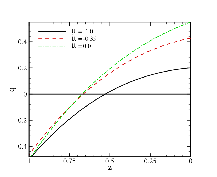
Figure 1: Acceleration parameter ($q=\ddot{a}/aH_{0}^{2}$) in the braneworld model as a function of redshift for various values of $\mu$. Here we chose $\Omega_{K}=0.0$, $\Omega_{m}=0.30$ and $\Omega_{A}=-0.70$.

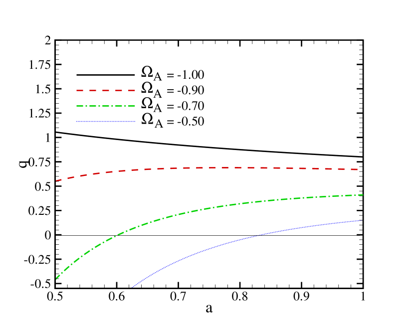
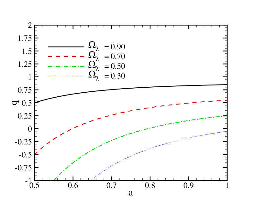
Figure 2: Upper panel shows acceleration parameter $(q=\ddot{a}/{H_{0}^{2}a})$ in the braneworld model as a function of scale factor for various values of $\Omega_{A}$ and $\mu=-0.40$. Lower panel corresponds to the same function for the flat $\Lambda$CDM. We chose the flat Universe.

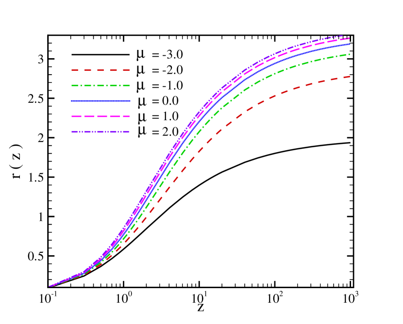
Figure 3: Comoving distance, $r(z;\Omega_{m},\Omega_{A},\mu)$ (in unit of $c/H_{0}$) as a function of redshift for various values of $\mu$. We fixed $\Omega_{K}=0.0$, $\Omega_{m}=0.3$ and $\Omega_{A}=-0.7$.

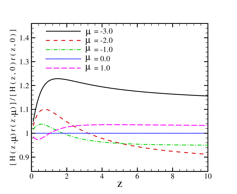
Figure 4: Alcock-Paczynski test comparing $\Delta z/{\Delta\theta}$ as a function of redshift for five different $\mu$ normalized to the case with $\Omega_{m}=0.30$ and $\Omega_{A}=-0.70$ and $\mu=0.0$ (flat Universe $\Omega_{K}=0$ and $\Lambda$CDM ).

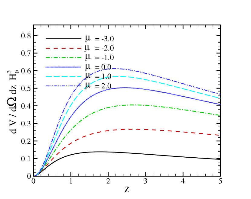
Figure 5: The comoving volume element in terms of redshift for various $\mu$ exponent. Increasing $\mu$ shifts the position of the maximum value of volume element to higher redshifts. We fixed $\Omega_{K}=0.0$.

Now an interesting question that arises is: can this model predict dynamics of the Universe? In other words, For what values of the free parameters, theoretical model is consistent with the observational tests?

In the forthcoming sections we will see what constraints to the described model are set by recent observations. As a matter of fact we examine the free parameters of model more carefully. Indeed we let the parameters scan their phase space and using likelihood statistics, the best fit values which maximize likelihood function will be retrieved.

3 Geometrical Effects of Braneworld Model

The cosmological observations are mainly affected by the background dynamics of the Universe. So before starting some main observational tests to explore braneworld cosmology we investigate how the free parameters of this model alter the background dynamics by using the measurable quantities introduced in this section. We believe they give deep insight throughout this model. For this purpose, we study the effect of the braneworld model on the geometrical parameters of the Universe all together.

3.1 comoving distance

The radial comoving distance is one of the basic parameters of cosmology. For an object with the redshift of $z$, using the null geodesics in the FRW metric, the comoving distance is obtained as:

$$r(z;\Omega_{m},\Omega_{A},\mu) = {1\over H_{0}\sqrt{|\Omega_{K}|}}\,{\cal F}\left(\sqrt{|\Omega_{K}|}\int_{0}^{z}\,{dz^{\prime}\over H(z^{\prime})/H_{0}}\right),$$

where

$${\cal F}(x) \equiv (x,\sin x,\sinh x)~{}{\rm for}~{}K=(0,1,-1)\,,$$ (28)

and $H(z;\Omega_{m},\Omega_{A},\mu)$ is given by equation (22).

By numerical integration of equation (3.1), the comoving distance in terms of redshift for different values of $\mu$ is shown in figure 3. Increasing the $\mu$ results in a longer comoving distance. According to this behavior by fine tuning the value of $\mu$ in addition to $\Omega_{A}$ and $\Omega_{m}$, one can expect to explain the observational results given by supernova as a standard candle to measure distance in the observational cosmology.

3.2 Angular Size

The apparent angular size of an object located at the cosmological distance is another important parameter that can be affected by the cosmological model during the history of the Universe. An object with the physical size of $D$ is related to the apparent angular size of $\theta$ by:

$$D=d_{A}\theta,$$ (29)

where $d_{A}=r(z;\Omega_{m},\Omega_{A},\mu)/(1+z)$ is the angular diameter distance. The main applications of equation (29) is on the measurement of the apparent angular size of acoustic peak on CMB and baryonic acoustic peak at the high and low redshifts, respectively. By measuring the angular size of an object in different redshifts (the so-called Alcock-Paczynski test) it is possible to probe the validity of braneworld model (C. Alcock el. al., 1979). The variation of apparent angular size $\Delta\theta$ in terms of $\Delta z$ is given by:

$${\Delta z\over\Delta\theta}=H(z;\Omega_{m},\Omega_{A},\mu)r(z;\Omega_{m},\Omega_{A},\mu).$$ (30)

Figure 4 shows $\Delta z/\Delta\theta$ in terms of redshift, normalized to the case with $\Omega_{m}=0.30$, $\Omega_{A}=-0.70$ and $\mu=0.0$ (flat Universe, $\Omega_{K}=0.0$). The advantage of Alcock-Paczynski test is that it is independent of standard candles and a standard ruler such as the size of baryonic acoustic peak can be used to constrain the braneworld model.

3.3 Comoving Volume Element

The comoving volume element is another geometrical parameter which is used in number-count tests such as lensed quasars, galaxies, or clusters of galaxies. The comoving volume element in terms of comoving distance and Hubble parameter is given by:

$$f(z;\Omega_{m},\Omega_{A},\mu) \equiv {dV\over dzd\Omega}$$ (31)

$$= r^{2}(z;\Omega_{m},\Omega_{A},\mu)/H(z;\Omega_{m},\Omega_{A},\mu).$$

According to figure 5, the comoving volume element becomes large for larger value of $\mu$ in the flat Universe.

4 Observational constraints on the model using background evolution of the Universe

In this section, at the beginning, we examine braneworld model by SNIa Gold sample and supernova Legacy Survey data. Then to make the model parameter intervals more confined, we will combine observational results of SNIa distance modules with power spectrum of cosmic microwave background radiation and baryon acoustic oscillation measured by Sloan Digital Sky survey. Table 1 shows different priors of the model parameters used in the likelihood analysis.

Parameter	Prior
$\Omega_{{\rm tot}}=\Omega_{m}-\Omega_{A}$	$-$	Free
$\Omega_{m}$	$[0.00,1.00]$	Top hat
$\Omega_{b}h^{2}$	$0.020\pm 0.005$	Top hat (BBN)
$\Omega_{A}$	$[-3.00,1.00]$	Top hat
$h$	$-$	Free
$\mu$	$-$	Free

Table 1: Priors of the parameter space, used in the likelihood analysis (A. Melchiorri el. al., 2003; W. L. Freedman el. al., 2001; X. Zhang el. al., 2005).

4.1 Supernova Type Ia: Gold and SNLS Samples

The Supernova Type Ia experiments provided the main evidence of the existence of dark energy. Since 1995 two teams of the High-Z Supernova Search and the Supernova Cosmology Project have discovered several type Ia supernovas at the high redshifts (S. Perlmutter el. al., 1999; B. P. Schmidt el. al., 1998). Recently, Riess et al.(2004) have announced the discovery of $16$ type Ia supernova with the Hubble Space Telescope. They determined the luminosity distance of these supernovas and with the previously reported algorithms, obtained a uniform $157$ Gold sample of type Ia supernovas (A. G. Riess el. al., 2004; J. L. Tonry el. al., 2003; B. J. Barris el. al., 2004). Recently a new data set of Gold sample with smaller systematic error containing $156$ Supernova Ia has been released (The Gold dataset, 2006). In this work we use this data set as new Gold sample SNIa.

More recently, the SNLS collaboration released the first year data of its planned five-year Supernova Legacy Survey(P. Astier el. al., 2005). An important aspect to be emphasized on the SNLS data is that they seem to be in a better agreement with WMAP results than the Gold sample (H. K. Jassal el. al., 2006). We compare the predictions of the braneworld model for apparent magnitude with new SNIa Gold sample and SNLS data set. The observations of supernova measure essentially the apparent magnitude $m$ including reddening, K correction, etc, which are related to the (dimensionless) luminosity distance, $D_{L}$, of an object at redshift $z$ through

$$m={\mathcal{M}}+5\log{D_{L}(z;\Omega_{m},\Omega_{A},\mu)},$$ (32)

where

$$D_{L}(z;\Omega_{m},\Omega_{A},\mu) = {(1+z)\over\sqrt{|\Omega_{K}|}}\,{\cal F}\left(\sqrt{|\Omega_{K}|}\int_{0}^{z}\,{dz^{\prime}H_{0}\over H(z^{\prime})}\right).$$ (33)

Also

$$\mathcal{M} = M+5\log{\left(\frac{c/H_{0}}{1\quad Mpc}\right)}+25,$$ (34)

where $M$ is the absolute magnitude. The distance modulus, $\Re$, is defined as

$$\Re\equiv m-M = 5\log{D_{L}(z;\Omega_{m},\Omega_{A},\mu)}$$ (35)

$$\quad+5\log{\left(\frac{c/H_{0}}{1\quad Mpc}\right)}+25,$$

or

$$\Re = 5\log{D_{L}(z;\Omega_{m},\Omega_{A},\mu)}+\bar{M}.$$ (36)

In order to compare the theoretical results with the observational data, we must compute the distance modulus, as given by equation (35). For this purpose, the first step is to compute the quality of the fitting through the least squared fitting quantity $\chi^{2}$ defined by:

$$\chi^{2}(\bar{M},\Omega_{m},\Omega_{A},\mu)=$$

$$\sum_{i}\frac{[\Re_{{\rm obs}}(z_{i})-\Re_{{\rm th}}(z_{i};\Omega_{m},\Omega_{A},\mu,\bar{M})]^{2}}{\sigma_{i}^{2}},$$ (37)

where $\sigma_{i}$ is the observational uncertainty in the distance modulus. To constrain the parameters of model, we use the Likelihood statistical analysis:

$${\cal L}(\bar{M},\Omega_{m},\Omega_{A},\mu)={\mathcal{N}}e^{-\chi^{2}(\bar{M},\Omega_{m},\Omega_{A},\mu)/2},$$ (38)

where ${\mathcal{N}}$ is a normalization factor. The parameter $\bar{M}$ is a nuisance parameter and should be marginalized (integrated out) leading to a new $\bar{\chi}^{2}$ defined as:

$$\bar{\chi}^{2}=-2\ln\int_{-\infty}^{+\infty}{\cal L}(\bar{M},\Omega_{m},\Omega_{A},\mu)d\bar{M}.$$ (39)

Using equations (4.1) and (39), we find

$$\bar{\chi}^{2}(\Omega_{m},\Omega_{A},\mu) = \chi^{2}(\bar{M}=0,\Omega_{m},\Omega_{A},\mu)$$ (40)

$$-\frac{B(\Omega_{m},\Omega_{A},\mu)^{2}}{C}+\ln(C/2\pi),$$

where

$$B(\Omega_{m},\Omega_{A},\mu)=$$

$$\sum_{i}\frac{[\Re_{{\rm obs}}(z_{i})-\Re_{{\rm th}}(z_{i};\Omega_{m},\Omega_{A},\mu,\bar{M}=0)]}{\sigma_{i}^{2}},$$ (41)

and

$$C=\sum_{i}\frac{1}{\sigma_{i}^{2}}.$$ (42)

Equivalent to marginalization is the minimization with respect to $\bar{M}$. One can show that $\chi^{2}$ can be expanded in $\bar{M}$ as (S. Nesseris el. al., 2004)

$$\chi^{2}_{\rm SNIa}(\Omega_{m},\Omega_{A},\mu) = \chi^{2}(\bar{M}=0,\Omega_{m},\Omega_{A},\mu)$$ (43)

$$-2\bar{M}B+\bar{M}^{2}C,$$

which has a minimum for $\bar{M}=B/C$:

$$\chi^{2}_{\rm SNIa}(\Omega_{m},\Omega_{A},\mu) = \chi^{2}(\bar{M}=0,\Omega_{m},\Omega_{A},\mu)$$ (44)

$$-\frac{B(\Omega_{m},\Omega_{A},\mu)^{2}}{C}.$$

Using equation (44) we can find the best fit values of model parameters as the values that minimize $\chi^{2}_{\rm SNIa}(\Omega_{m},\Omega_{A},\mu)$. The best fit values for the parameters of model by using supernova data are $\Omega_{m}=0.51^{+0.10}_{-0.30}$, $\Omega_{A}=-0.75_{-1.41}^{+0.32}$ and $\mu=0.76^{+7.24}_{-1.95}$ with $\chi^{2}_{min}/N_{d.o.f}=0.92$ at $1\sigma$ level of confidence. These values imply that $\Omega_{K}=-0.26_{-1.44}^{+0.33}$. The best fit values for the parameters of model by using SNLS supernova data are $\Omega_{m}=0.06^{+0.44}_{-0.06}$, $\Omega_{A}=-1.84_{-0.59}^{+1.58}$ and $\mu=-1.34^{+7.34}_{-0.10}$ with $\chi^{2}_{min}/N_{d.o.f}=0.87$ at $1\sigma$ level of confidence. The corresponding value of $\Omega_{K}$ at $1\sigma$ confidence level is $\Omega_{K}=-0.90^{+1.64}_{-0.59}$. Figures 6 and 7 show the comparison of the theoretical prediction of distance modulus by using the best fit values of model parameters and observational values from new Gold sample and SNLS supernova, respectively. Figures 8 and 9 show relative likelihood for free parameters of brane model.

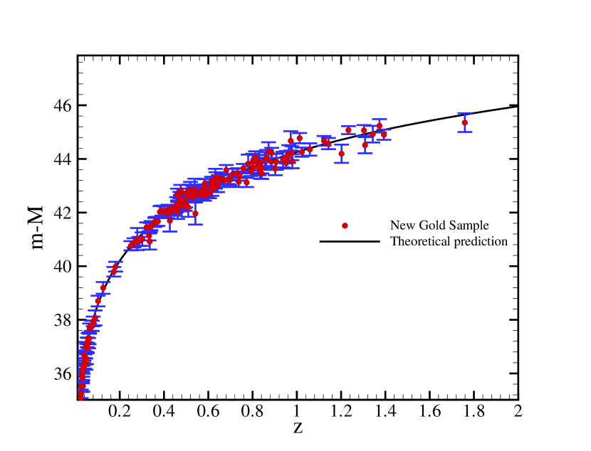
Figure 6: Distance modulus of the SNIa new Gold sample in terms of redshift. Solid line shows the best fit values with the corresponding parameters of $H_{0}=63.66$, $\Omega_{m}=0.51^{+0.10}_{-0.30}$, $\Omega_{A}=-0.75_{-1.41}^{+0.32}$ and $\mu=0.76_{-1.95}^{+7.24}$ in $1\sigma$ level of confidence with $\chi^{2}_{min}/N_{d.o.f}=0.92$ for brane world model.

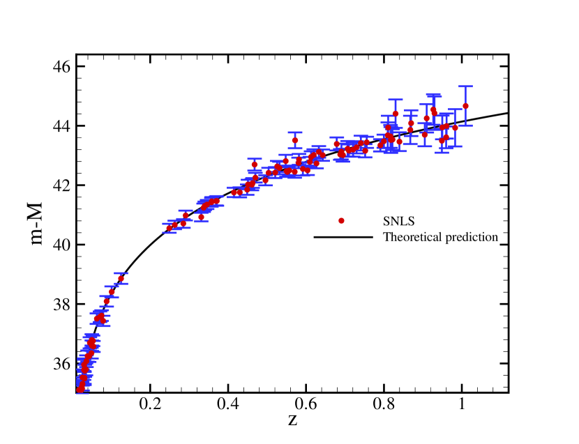
Figure 7: Distance modulus of the SNLS supernova data in terms of redshift. Solid line shows the best fit values with the corresponding parameters of $H_{0}=69.38$, $\Omega_{m}=0.06^{+0.44}_{-0.06}$, $\Omega_{A}=-1.84_{-0.59}^{+1.58}$ and $\mu=-1.34^{+7.34}_{-0.10}$ in $1\sigma$ level of confidence with $\chi^{2}_{min}/N_{d.o.f}=0.87$ for brane world model.

4.2 Combined analysis: SNIa$+$CMB$+$SDSS

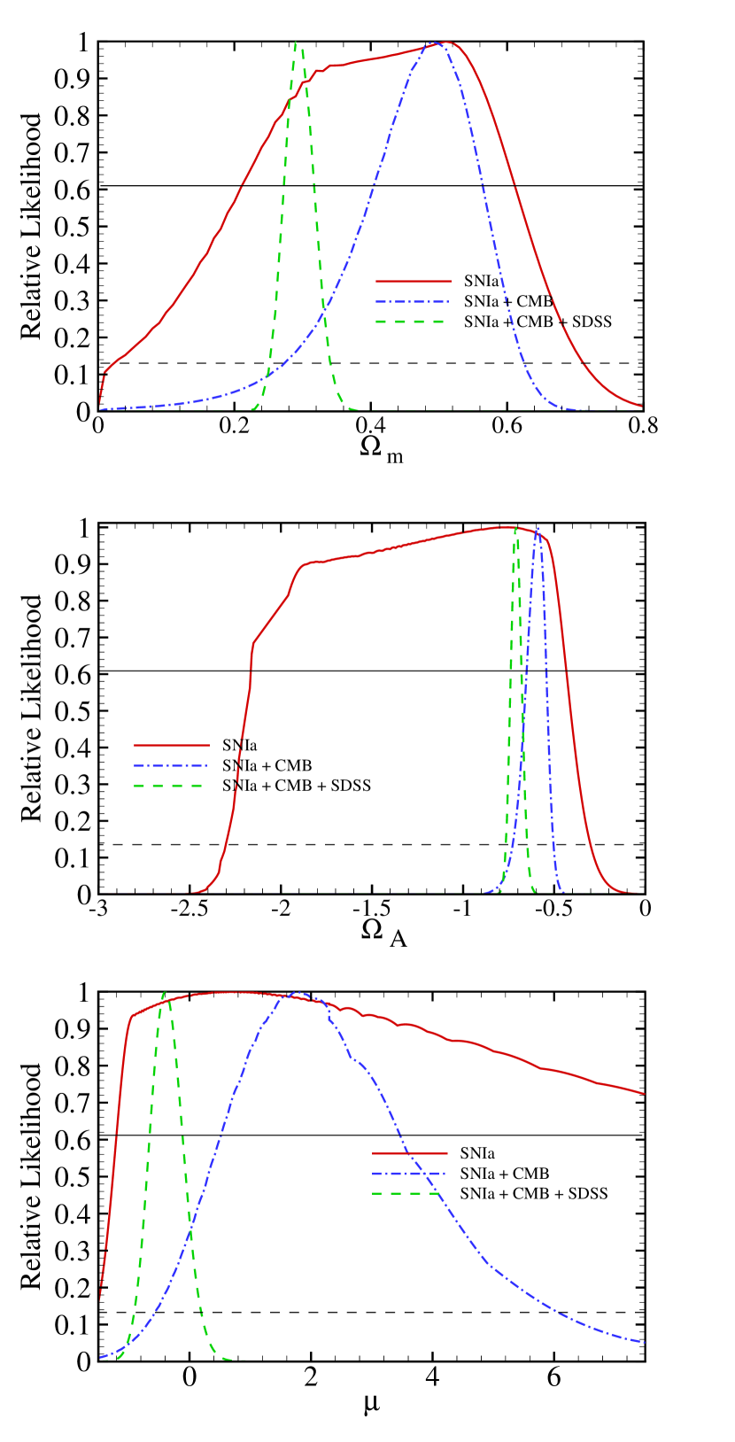
Figure 8: Marginalized likelihood functions of three parameters of model ($\Omega_{m}$, $\Omega_{A}$ and $\mu$). The solid line corresponds to the likelihood function of fitting the model with SNIa data (new Gold sample), the dashdot line with the joint SNIa$+$CMB data and dashed line corresponds to SNIa$+$CMB$+$SDSS. The intersections of the curves with the horizontal solid and dashed lines give the bounds with $1\sigma$ and $2\sigma$ level of confidence respectively.

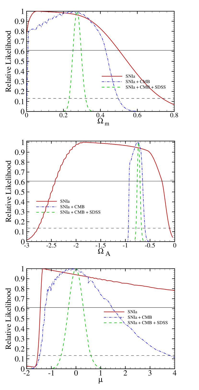
Figure 9: Marginalized likelihood functions of three parameters of a braneworld model ($\Omega_{m}$, $\Omega_{A}$ and $\mu$). The solid line corresponds to the likelihood function of fitting the model with SNIa data (SNLS), the dashdot line with the joint SNIa$+$CMB data and dashed line corresponds to SNIa$+$CMB$+$SDSS. The intersections of the curves with the horizontal solid and dashed lines give the bounds with $1\sigma$ and $2\sigma$ level of confidence respectively.

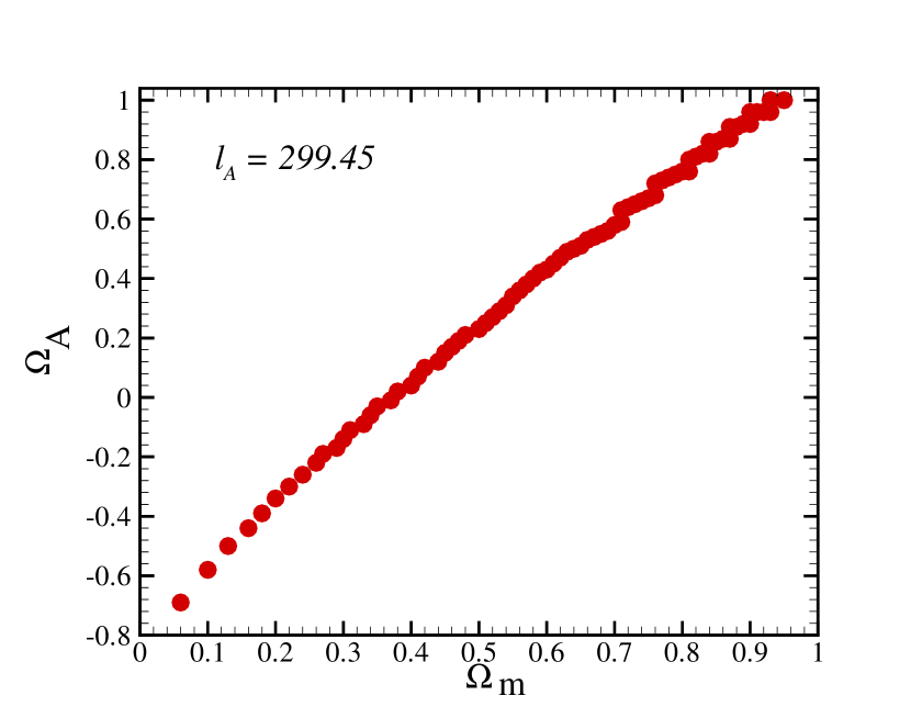
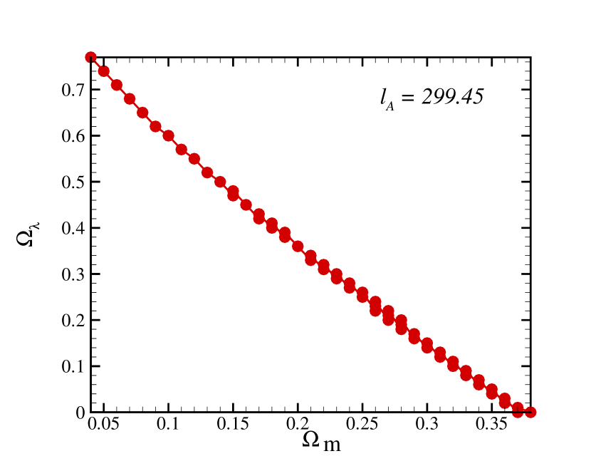
Figure 10: Constant acoustic angular scale in the joint space of $\Omega_{m}$ and $\Omega_{A}$ (upper panel). Lower panel shows dependence of acoustic angular scale on the $\Omega_{m}$ and cosmological constant.

To obtain more confined acceptable intervals of model free parameters, now we combine SNIa data (from SNIa new Gold sample and SNLS) with CMB data from the WMAP and recently observed baryonic peak from the SDSS. We also examine the peaks positions of power spectrum in addition to the common shift parameter.

Before last scattering, the photons and baryons are tightly coupled by Compton scattering and behave as a fluid. The oscillations of this fluid, occurring as a result of the balance between the gravitational interactions and the photon pressure, lead to the familiar spectrum of peaks and troughs in the averaged temperature anisotropy spectrum which we measure today. The odd and even peaks correspond to maximum compression of the fluid and to rarefaction, respectively (Wayne Hu el. al., 1997). In an idealized model of the fluid, there is an analytic relation for the location of the $m$-th peak: $l_{m}\approx ml_{A}$ (W. Hu el. al., 1995; Hu, W. et. al., 2001) where $l_{A}$ is the acoustic scale which may be calculated analytically and depends on both pre- and post-recombination physics as well as the geometry of the Universe. The acoustic scale corresponds to the Jeans length of photon-baryon structures at the last scattering surface some $\sim 379$ Kyr after the Big Bang (D. N. Spergel el. al., 2003a). The apparent angular size of acoustic peak can be obtained by dividing the comoving size of sound horizon at the decoupling epoch $r_{s}(z_{dec})$ by the comoving distance of observer to the last scattering surface $r(z_{dec})$

$$\theta_{A}=\frac{\pi}{l_{A}}\equiv{{r_{s}(z_{dec})}\over r(z_{dec})}.$$ (45)

The size of sound horizon at the numerator of equation (45) corresponds to the distance that a perturbation of pressure can travel from the beginning of the Universe up to the last scattering surface and is given by

$$r_{s}(z_{dec};\Omega_{m},\Omega_{A},\mu)$$

$$={1\over H_{0}\sqrt{|\Omega_{K}|}}\times{\cal F}\left(\sqrt{|\Omega_{K}|}\int_{z_{dec}}^{\infty}{v_{s}(z^{\prime})dz^{\prime}\over H(z^{\prime})/H_{0}}\right),$$ (46)

where $v_{s}(z)^{-2}=3+9/4\times\rho_{b}(z)/\rho_{rad}(z)$ is the sound velocity in the unit of speed of light from the big bang up to the last scattering surface (M. Doran el. al., 2001; W. Hu el. al., 1995) and the redshift of the last scattering surface, $z_{dec}$, is given by (W. Hu el. al., 1995):

$$z_{dec} = 1048\left[1+0.00124(\omega_{b})^{-0.738}\right]\left[1+g_{1}(\omega_{m})^{g_{2}}\right],$$

$$g_{1} = 0.0783(\omega_{b})^{-0.238}\left[1+39.5(\omega_{b})^{0.763}\right]^{-1},$$

$$g_{2} = 0.560\left[1+21.1(\omega_{b})^{1.81}\right]^{-1},$$ (47)

where $\omega_{m}\equiv\Omega_{m}h^{2}$, $\omega_{b}\equiv\Omega_{b}h^{2}$ and $\rho_{rad}$ is the radiation density. $\Omega_{b}$ is relative baryonic density to the critical density at the present time. Changing the parameters of the model can change the size of apparent acoustic peak and subsequently the position of $l_{A}\equiv\pi/\theta_{A}$ in the power spectrum of temperature fluctuations at the last scattering surface. The simple relation $l_{m}\approx ml_{A}$ however does not hold very well for the peaks although it is better for higher peaks (Hu, W. et. al., 2001; Michael Doran el. al., 2001). Driving effects from the decay of the gravitational potential as well as contributions from the Doppler shift of the oscillating fluid introduce a shift in the spectrum. A good parameterization for the location of the peaks and troughs is given by (Hu, W. et. al., 2001; Michael Doran el. al., 2001)

$$l_{m}=l_{A}(m-\phi_{m}),$$ (48)

where $\phi_{m}$ is phase shift determined predominantly by pre-recombination physics, and are independent of the geometry of the Universe. The location of acoustic peaks can be determined in model by equation (48) with $\phi_{m}(\omega_{m},\omega_{b})$. Doran et. al. (Michael Doran el. al., 2001), have recently shown that the first and third phase shifts are approximately model independent. The values of these shift parameters have been reported as: $\phi_{1}(\omega_{m},\omega_{b})\simeq 0.27$ and $\phi_{3}(\omega_{m},\omega_{b})\simeq 0.341$ (Hu, W. et. al., 2001; W. J. Percival et. al., 2002; Michael Doran el. al., 2001). According to the WMAP observations: $l_{1}=220.1\pm 0.8$ and $l_{3}=809\pm 7$, so the corresponding observational values of $l_{A}^{\rm obs}$ read as:

$$l_{A}^{\rm obs}|_{l_{1}} = \frac{l_{1}}{(1-\phi_{1})}=299.45\pm 2.67,$$ (49)

$$l_{A}^{\rm obs}|_{l_{3}} = \frac{l_{3}}{(3-\phi_{3})}=304.24\pm 2.63,$$ (50)

their Likelihood statistics are as follows:

$$\chi_{l_{1}}^{2}=\frac{\left[l_{A}^{\rm obs}|_{l_{1}}-l_{A}^{\rm th}|_{l_{1}}\right]^{2}}{\sigma_{1}^{2}},$$ (51)

and

$$\chi_{l_{3}}^{2}=\frac{\left[l_{A}^{\rm obs}|_{l_{3}}-l_{A}^{\rm th}|_{l_{3}}\right]^{2}}{\sigma_{3}^{2}},$$ (52)

because of weak dependency of phase shift to the cosmological model usually another model independent parameter which is so-called shift parameter ${\cal R}$ from CMB observation as

$${\cal R}\propto\frac{l_{1}^{flat}}{l_{1}},$$ (53)

are used as another observational test. Where $l_{1}^{flat}$ corresponds to the flat pure-CDM model with $\Omega_{m}=1.0$ and the same $\omega_{m}$ and $\omega_{b}$ as the original model. It is easily shown that shift parameter is as follows (J. R. Bond el. al., 1997)

$${\cal R}=\sqrt{\Omega_{m}}\frac{D_{L}(z_{dec},\Omega_{m},\Omega_{A},\mu)}{(1+z_{dec})}.$$ (54)

The observational results of CMB experiments correspond to a shift parameter of ${\cal R}=1.716\pm 0.062$ (given by WMAP, CBI, ACBAR) (D. N. Spergel el. al., 2003a; T. J. Pearson el. al., 2003; C. L. Kuo et. al., 2004). One of the advantages of using the parameter ${\cal R}$ is its independency of Hubble constant. In order to put constraint on the model from CMB, we compare the observed shift parameter with that of model using likelihood statistic as (J. R. Bond el. al., 1997; A. Melchiorri el. al., 2003; C. J. Odman et. al., 2003)

$${\cal{L}}\sim e^{-\chi_{\rm CMB}^{2}/2},$$ (55)

where

$$\chi_{\rm CMB}^{2}=\frac{\left[{\cal R}_{{\rm obs}}-{\cal R}_{{\rm th}}\right]^{2}}{\sigma_{\rm CMB}^{2}},$$ (56)

where ${\cal R}_{{\rm th}}$ and ${\cal R}_{{\rm obs}}$ are determined using equation (54) and given by observation, respectively. Figure 10 shows constant value of $l_{A}$ in the joint space parameters $(\Omega_{m},\Omega_{A})$ and $(\Omega_{m},\Omega_{\lambda})$ for the braneworld and the $\Lambda$CDM model, respectively. Increasing (decreasing) $\Omega_{A}$ ($\Omega_{\lambda}$) leads to an increasing in the value of present matter density to make constant value for $l_{A}$. What we found is in agreement with figure 2.

Another robust observational approach to investigate cosmological models is inferring the behavior of the matter power spectrum and time evolution of gravitational clustering in both linear and nonlinear regimes. The simplest things to do are solving the relevant Boltzmann and Einestian equations for various matter contents in the Universe (S. Dodelson, 2003). Matter power spectrum and other non-linear effects can be a special tools to discriminate various models as well as to make more confined acceptable range for their free parameters (see (C. P. Ma et. al., 1999; Z. Ma, 2006; T. koivisto, 2006; G. Olivares et. al., 2005, 2006; S. Lee et. al., 2006; V. R. Eke et. al., 2001; D. Jeong and E. Komatsu, 2006; U. Seljak and M. Zaldarriaga, 1999; D. H. Rudd et. al., 2007; A. Loeb and M. Zaldarriaga, 2005; R. R. R. Reis et. al., 2005; G. Olivares et. al., 2005, 2006; P. J. E. Peebles, 2003; L. P. Chimento and D. Pavon, 2006; L. Amendola, 2000; L. Amendola et. al., 2001; L. Amendola, 2002; L. Amendola et. al., 2003b) for recent reviews). The conventional form of matter power spectrum at the late time is (S. Dodelson, 2003):

$$P(k,a)=2\pi^{2}\delta_{H}^{2}T(k)^{2}\frac{k^{n}}{H_{0}^{3+n}}\left(\frac{D(a)}{D(a=1)}\right)^{2}$$ (57)

where $n$ is the spectral index of the primordial adiabatic density perturbations, $T(k)$ is transfer function determines the evolution of potential in the radiation-matter equality epoch and in the late time matter density fluctuations govern by so-called growth function, $D(a)$. $\delta_{H}$ is also given by initial condition in the context of inflation. $k$ is the wave-number of fluctuations in the Fourier space. Generally, it is well known that if any interaction between matter and dark energy in addition to the new kind of matter which are the responsible for the background dynamics of the Universe to be existed, they alter the matter power spectrum through the three following effects: The first one is that, the Hubble parameter in different models causes various dynamics for the background evolution (e.g. in our model is given by equation (22)) as well as power spectrum. The second effect is due to the inverse proportional of power spectrum to the matter density for a fixed potential, so any variation in the present value of matter density causes the smaller or larger amplitude for power spectrum. Third effect is related to the fact that in different cosmological models, the matter-radiation equality epoch, $a_{eq}$ and subsequently the value of $k_{eq}$ change, so the turning over point in the power spectrum would be reformed.

Here instead of observational constraint using matter power spectrum we used the weakly model independent constraint by Baryon acoustic oscillation and ignore any non-linear effects (E. V. Linder, 2005, 2003). Recently using the observations of large scale structures from the Sloan Digital Sky Survey (SDSS) M. Tegmark, et al. (2004a); M. Tegmark, R. Michael Blanton et al. (2004b) and Two Degree Field Galaxy Redshift Survey (2dFGRS) M. Tegmark, et al. (2002), one can explore the validity of cosmological models.

The large scale correlation function measured from $46,748$ Luminous Red Galaxies (LRG) spectroscopic sample of the SDSS includes a clear peak at about $100$ Mpc $h^{-1}$ (D. J. Eisenstein el. al., 2005). This peak was identified with the expanding spherical wave of baryonic perturbations originating from acoustic oscillations at recombination. The comoving scale of this shell at recombination is about $150$Mpc in radius. In other words, this peak has an excellent match to the predicted shape and the location of the imprint of the recombination-epoch acoustic oscillation on the low-redshift clustering matter (D. J. Eisenstein el. al., 2005). Recently E. V. Linder has shown in detail some systematic uncertainties for baryon acoustic oscillation (E. V. Linder, 2005, 2003). Nonlinear mode coupling related to this fact that ever though baryon acoustic oscillation is mostly contributed by linear scale, but the influence of non-linear collapsing has quite broad kernel. In other words, one might say that baryon acoustic oscillation are $90-99\%$ linear in comparison to the CMB which is $99.99\%$ linear, so this difference may affect on various models in different way. Careful works to constrain on the free parameters of underlying model needs to be carried out the effect of non-linear mode coupling in the results of constraint by SDSS observation. Nevertheless, roughly speaking regards the acceptance intervals for free parameter cover the real intervals determined by assuming nonlinearity mode for SDSS observation (W. Hu et. al., 1996; D. J. Eisenstein et. al., 1998; M. Amarzguioui et. al., 2005; D. Eisenstein et. al., 2004).

A dimensionless and independent of $H_{0}$ version of SDSS observational parameter is

$${\cal A} = D_{V}(z_{\rm sdss})\frac{\sqrt{\Omega_{m}H_{0}^{2}}}{z_{\rm sdss}}$$

$$= \sqrt{\Omega_{m}}\left[\frac{H_{0}D_{L}^{2}(z_{\rm sdss};\Omega_{m},\Omega_{A},\mu)}{H(z_{\rm sdss};\Omega_{m},\Omega_{A},\mu)z_{\rm sdss}^{2}(1+z_{\rm sdss})^{2}}\right]^{1/3},$$

where $D_{V}(z_{\rm sdss})$ is characteristic distance scale of the survey with the mean of redshift $z_{\rm sdss}$ (D. J. Eisenstein el. al., 2005; C. Blake el. al., 2003; S. Nesseris el. al., 2007). We use the robust constraint on the braneworld model using the value of ${\cal A}=0.469\pm 0.017$ from the LRG observation at $z_{\rm sdss}=0.35$ (D. J. Eisenstein el. al., 2005; D. Eisenstein et. al., 2004). This observation permits the addition of one more term in the $\chi^{2}$ of equations (44) and (56) to be minimized with respect to $H(z)$ model parameters. This term is

$$\chi_{\rm SDSS}^{2}=\frac{\left[{\cal A}_{\rm obs}-{\cal A}_{\rm th}\right]^{2}}{\sigma_{\rm SDSS}^{2}}.$$ (59)

This is the third observational constraint for our analysis.

In the rest of this subsection we perform a combined analysis of SNIa, CMB and SDSS to constrain the parameters of the braneworld model by minimizing the combined $\chi^{2}=\chi^{2}_{\rm{SNIa}}+\chi^{2}_{{\rm CMB}}+\chi^{2}_{{\rm SDSS}}$. The best values of the model parameters from the fitting with the corresponding error bars from the likelihood function marginalizing over the Hubble parameter in the multidimensional parameter space are: $\Omega_{m}=0.29_{-0.02}^{+0.03}$, $\Omega_{A}=-0.71_{-0.03}^{+0.03}$ and $\mu=-0.40^{+0.28}_{-0.26}$ at $1\sigma$ confidence level with $\chi^{2}_{min}/N_{d.o.f}=0.93$ demonstrated $\Omega_{K}=+0.00_{-0.04}^{+0.04}$ . The Hubble parameter corresponding to the minimum value of $\chi^{2}$ is $H_{0}=62.72$. Here we obtain an age of $14.82_{-0.44}^{+0.55}$ Gyr for the Universe (see section V for more details). Using the SNLS data, the best fit values of model parameters are: $\Omega_{m}=0.27_{-0.02}^{+0.02}$ $\Omega_{A}=-0.74_{-0.02}^{+0.04}$ and $\mu=0.00^{+0.30}_{-0.30}$ at $1\sigma$ confidence level with $\chi^{2}_{min}/N_{d.o.f}=0.86$, states $\Omega_{K}=-0.01_{-0.03}^{+0.04}$. Age of Universe calculating with the best fit parameters is $14.05_{-0.45}^{+0.43}$ (see next section). Tables 2 and 3 give the best fit values for the free parameters and age of Universe computing with these values. Joint confidence intervals in free parameter spaces are shown in figures 11-16.

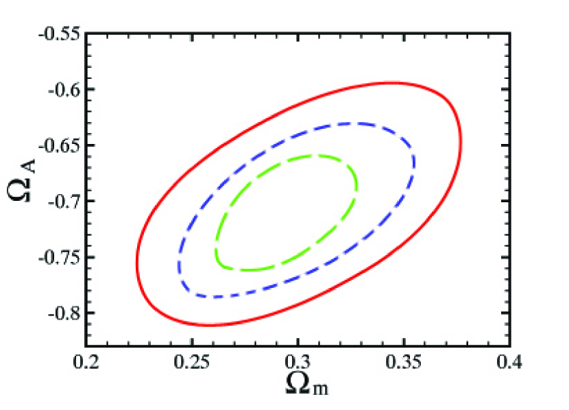
Figure 11: Joint confidence intervals of $\Omega_{m}$ and $\Omega_{A}$, fitted with SNIa new Gold sample$+$CMB$+$SDSS. Solid line, dashed line and long dashed line correspond to $3\sigma$, $2\sigma$ and $1\sigma$ level of confidence, respectively.

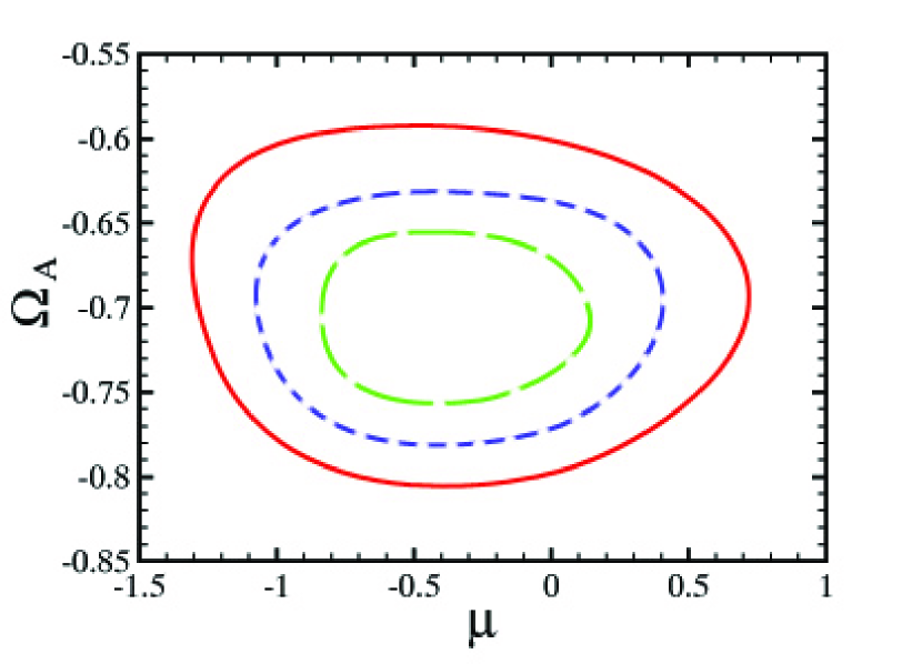
Figure 12: Joint confidence intervals of $\mu$ and $\Omega_{A}$, fitted with SNIa new Gold sample$+$CMB$+$SDSS. Solid line, dashed line and long dashed line correspond to $3\sigma$, $2\sigma$ and $1\sigma$ level of confidence, respectively.

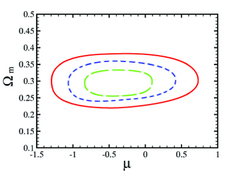
Figure 13: Joint confidence intervals of $\mu$ and $\Omega_{m}$, fitted with SNIa new Gold sample$+$CMB$+$SDSS. Solid line, dashed line and long dashed line correspond to $3\sigma$, $2\sigma$ and $1\sigma$ level of confidence, respectively.

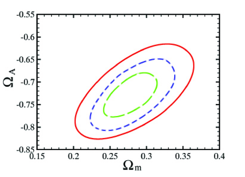
Figure 14: Joint confidence intervals of $\Omega_{m}$ and $\Omega_{A}$, fitted with SNIa SNLS$+$CMB$+$SDSS. Solid line, dashed line and long dashed line correspond to $3\sigma$, $2\sigma$ and $1\sigma$ level of confidence, respectively.

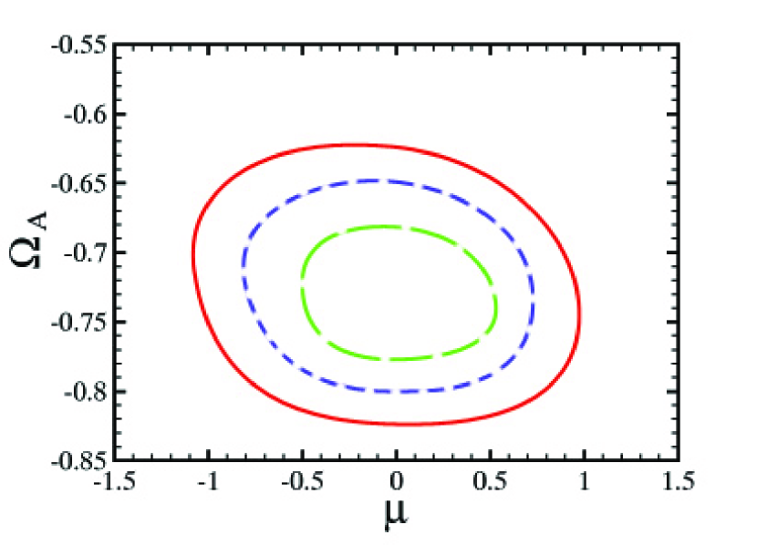
Figure 15: Joint confidence intervals of $\mu$ and $\Omega_{A}$, fitted with SNIa SNLS$+$CMB$+$SDSS. Solid line, dashed line and long dashed line correspond to $3\sigma$, $2\sigma$ and $1\sigma$ level of confidence, respectively.

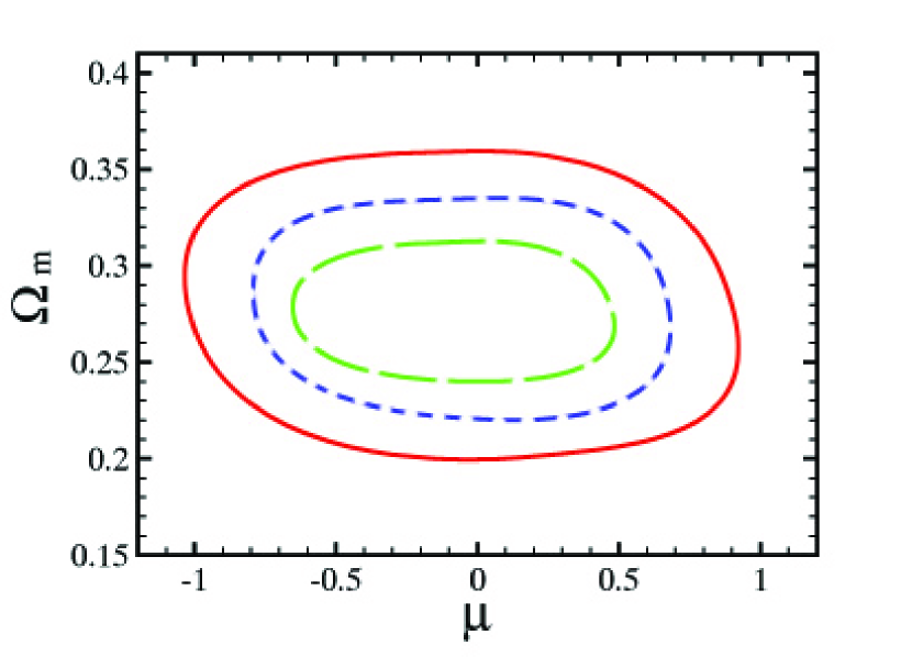
Figure 16: Joint confidence intervals of $\mu$ and $\Omega_{m}$, fitted with SNIa SNLS$+$CMB$+$SDSS. Solid line, dashed line and long dashed line correspond to $3\sigma$, $2\sigma$ and $1\sigma$ level of confidence, respectively.

Observation	$\Omega_{m}$	$\Omega_{A}$	$\mu$
	$0.51^{+0.10}_{-0.30}$	$-0.75_{-1.41}^{+0.32}$	$0.76^{+7.24}_{-1.95}$
SNIa(new Gold)
	$0.51^{+0.14}_{-0.54}$	$-0.75_{-1.55}^{+0.45}$	$0.76^{+15.24}_{-2.27}$
SNIa(new Gold)+CMB	$0.49^{+0.07}_{-0.08}$	$-0.59^{+0.05}_{-0.06}$	$-1.76^{+1.72}_{-1.31}$
	$0.49^{+0.14}_{-0.21}$	$-0.59^{+0.09}_{-0.14}$	$-1.76^{+4.28}_{-2.32}$
SNIa(new Gold)+	$0.29^{+0.03}_{-0.02}$	$-0.71^{+0.03}_{-0.03}$	$-0.40^{+0.28}_{-0.26}$
CMB+SDSS
	$0.29^{+0.05}_{-0.04}$	$-0.71^{+0.06}_{-0.06}$	$-0.40^{+0.58}_{-0.56}$
	$0.06^{+0.44}_{-0.06}$	$-1.84^{+1.58}_{-0.59}$	$-1.34^{+7.34}_{-0.10}$
SNIa (SNLS)
	$0.06^{+0.68}_{-0.06}$	$-1.84^{+1.73}_{-0.94}$	$-1.34^{+17.34}_{-0.22}$
SNIa(SNLS)+CMB	$0.23^{+0.20}_{-0.23}$	$-0.76^{+0.11}_{-0.16}$	$-0.26^{+1.72}_{-1.00}$
	$0.23^{+0.27}_{-0.23}$	$-0.76^{+0.16}_{-0.17}$	$-0.26^{+4.04}_{-1.22}$
SNIa(SNLS)+	$0.27^{+0.02}_{-0.02}$	$-0.74^{+0.04}_{-0.02}$	$0.00^{+0.30}_{-0.30}$
CMB+SDSS
	$0.27^{+0.05}_{-0.04}$	$-0.74^{+0.07}_{-0.05}$	$0.00^{+0.60}_{-0.60}$

Table 2: The best fit values for the parameters of the model using SNIa from new Gold sample and SNLS data, SNIa+CMB and SNIa+CMB+SDSS experiments at one and two $\sigma$ confidence level.

Observation	$\Omega_{K}$	Age (Gyr)
SNIa(new Gold)	$-0.26^{+0.33}_{-1.44}$	$13.44^{+2.10}_{-7.13}$
SNIa(new Gold)+CMB	$+0.01^{+0.09}_{-0.10}$	$13.53^{+0.85}_{-1.18}$
SNIa(new Gold)+	$+0.00^{+0.04}_{-0.04}$	$14.82^{+0.55}_{-0.44}$
CMB+SDSS
SNIa (SNLS)	$-0.90^{+1.64}_{-0.59}$	$14.38^{+2.00}_{-1.81}$
SNIa(SNLS)+CMB	$-0.01^{+0.23}_{-0.28}$	$14.38^{+3.03}_{-14.38}$
SNIa(SNLS)+	$-0.01^{+0.04}_{-0.03}$	$14.05^{+0.43}_{-0.45}$
CMB+SDSS

Table 3: The best values for the curvature of the brane model with the corresponding age for the Universe from fitting with SNIa from new Gold sample and SNLS data, SNIa+CMB and SNIa+CMB+SDSS experiments at one and two $\sigma$ confidence level.

	LBDS	LBDS	APM
Observation	$53$W$069$	$53$W$091$	$08279+5255$
	$z=1.43$	$z=1.55$	$z=3.91$
SNIa (new Gold)	$1.00^{+0.10}_{-0.75}$	$1.06^{+0.10}_{-0.76}$	$0.65^{+0.14}_{-0.41}$
SNIa(new Gold)+CMB	$0.98^{+0.07}_{-0.10}$	$1.04^{+0.07}_{-0.10}$	$0.65^{+0.14}_{-0.07}$
SNIa(new Gold)+CMB	$1.22^{+0.06}_{-0.04}$	$1.31^{+0.06}_{-0.05}$	$0.84^{+0.17}_{-0.04}$
+SDSS
SNIa (SNLS)	$2.33^{+1.15}_{-1.13}$	$2.55^{+1.35}_{-1.31}$	$1.91^{+1.70}_{-1.65}$
SNIa(SNLS)+CMB	$1.23^{+0.31}_{-1.23}$	$1.32^{+0.34}_{-1.32}$	$0.85^{+0.28}_{-0.85}$
SNIa(SNLS)+CMB	$1.16^{+0.04}_{-0.05}$	$1.24^{+0.04}_{-0.05}$	$0.79^{+0.16}_{-0.04}$
+SDSS

Table 4: The value of $\tau$ for three high redshift objects, using the parameters of the model derived from fitting with the observations.

5 Age of Universe

The age of Universe integrated from the big bang up to now in terms of free parameters of the braneworld model is given by

$$t_{0}(\Omega_{m},\Omega_{A},\mu)=\int_{0}^{t_{0}}\,dt$$

$$={1\over H_{0}\sqrt{|\Omega_{K}|}}\,{\cal F}\left(\sqrt{|\Omega_{K}|}\int_{0}^{\infty}{dz^{\prime}H_{0}\over(1+z^{\prime})H(z^{\prime})}\right).$$ (60)

Figure 17 shows the dependency of $H_{0}t_{0}$ (Hubble parameter times the age of Universe) on $\Omega_{A}$ and $\mu$ for a flat Universe. Obviously increasing $\Omega_{A}$ and $\mu$ result in a shorter and longer age for the Universe, respectively. As a matter of fact, according to the equation (22), $\Omega_{A}$ behaves as inverse role of dark energy in the $\Lambda$CDM scenario and $\mu$ has the inverse role of $w$ in the $\Lambda$CDM (see Figures 17 and 18).

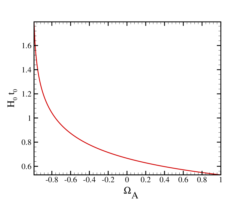
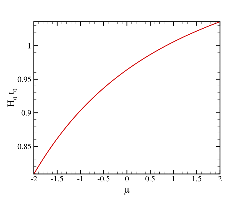
Figure 17: $H_{0}t_{0}$ (age of Universe times the Hubble constant at the present time) as a function of $\Omega_{A}$ (upper panel) for a flat Universe and typical value of $\mu=-0.40$. Increasing $\Omega_{A}$ gives a shorter age for the Universe. Lower panel shows the same function versus $\mu$ for the case $\Omega_{m}=0.30$, $\Omega_{A}=-0.70$ (flat Universe).

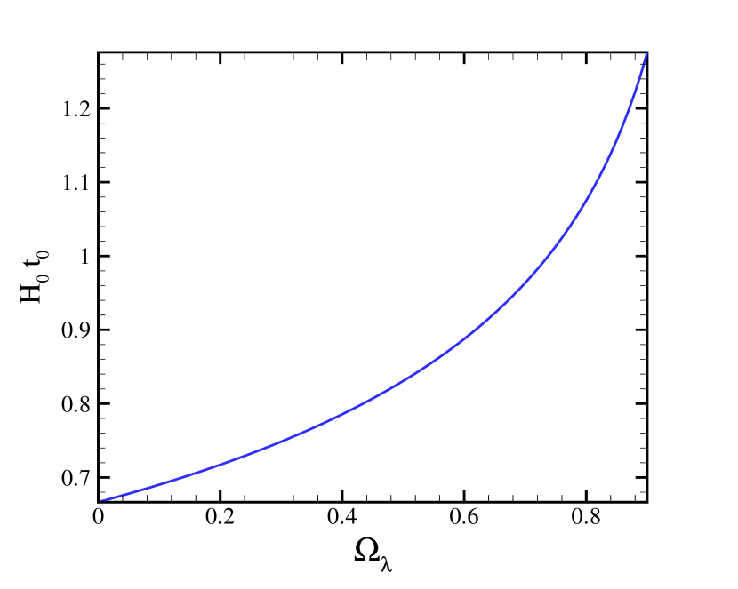
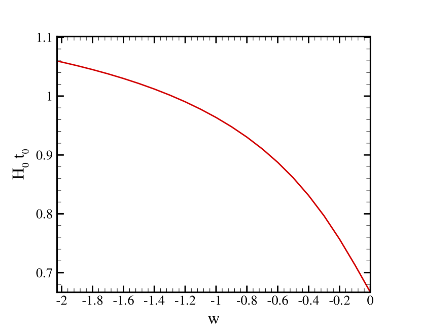
Figure 18: $H_{0}t_{0}$ (age of Universe times the Hubble constant at the present time) versus $\Omega_{\lambda}$ (upper panel) in the $\Lambda$CDM model for the case $\Omega_{K}=0.0$ and $w=-1.0$. Lower panel shows $H_{0}t_{0}$ as a function of present equation of state, $w$, in the $\Lambda$CDM model with the typical values $\Omega_{m}=0.30$ and $\Omega_{\lambda}=0.70$.

The “age crisis” is one the main reasons of the acceleration phase of the Universe. The problem is that the Universe’s age in the Cold Dark Matter (CDM) Universe is less than the age of old stars in it. Studies on the old stars (E. Carretta el. al., 2000) suggest an age of $13^{+4}_{-2}$ Gyr for the Universe. Richer et. al. (H. B. Richer el. al., 2002) and Hasen et. al. (B. M. S. Hansen el. al., 2002) also proposed an age of $12.7\pm 0.7$ Gyr, using the white dwarf cooling sequence method (for full review of the cosmic age see (D. N. Spergel el. al., 2003a)). Table 3 shows that age of the Universe from the combined analysis of SNIa$+$CMB$+$SDSS is $14.82_{-0.44}^{+0.55}$ Gyr and $14.05_{-0.45}^{+0.43}$ Gyr for new Gold sample and SNLS data, respectively, while $\Lambda$CDM implies $13.7\pm 0.2$Gyr (D. N. Spergel el. al., 2003a). These values are in agreement with the age of old stars (E. Carretta el. al., 2000; L. M. Krauss et. al., 2001; B. Chaboyer et. al., 2002).

To do another consistency test, we compare the age of Universe derived from this model with the age of old stars and Old High Redshift Galaxies (OHRG) in various redshifts. Here we consider three OHRG for comparison with the braneworld model, namely the LBDS $53$W$091$, a $3.5$-Gyr old radio galaxy at $z=1.55$ (J. Dunlop el. al., 1996; H. Spinrard, 1997), the LBDS $53$W$069$ a $4.0$-Gyr old radio galaxy at $z=1.43$ (J. Dunlop, 1999) and a quasar, APM $08279+5255$ at $z=3.91$ with an age of $t=2.1_{-0.1}^{+0.9}$Gyr (G. Hasinger el. al., 2002; S. Komossa et. al., 2002). The later has once again led to the ”age crisis”. An interesting point about this quasar is that it cannot be accommodated in the $\Lambda$CDM model (D. Jain. el. al., 2005). In order to quantify the age-consistency test we introduce the expression $\tau$ as:

$$\tau=\frac{t(z;\Omega_{m},\Omega_{A},\mu)}{t_{{\rm obs}}}=\frac{t(z;\Omega_{m},\Omega_{A},\mu)H_{0}}{t_{{\rm obs}}H_{0}},$$ (61)

where $t(z)$ is the age of Universe, obtained from the equation (17) and $t_{obs}$ is an estimation for the age of old cosmological object. In order to have a compatible age for the Universe we should have $\tau>1$. Table 4 reports the value of $\tau$ for three mentioned OHRG with various observations. We see that the parameters of braneworld model from the combined observations provide a compatible age for the Universe, compared to the age of old objects, also in addition, SNLS data result in a shorter age for the Universe. Once again for the braneworld model, APM $08279+5255$ at $z=3.91$ has a longer age than the Universe but gives better result than most cosmological models investigated before (L. F. Miranda et al., 2001; S. Rahvar el. al., 2007; D. Jain. el. al., 2005).

6 conclusions and discussions

The impressive amount of data indicating a spatially flat Universe in accelerated expansion has posed the problem of dark energy and stimulated the search for cosmological models which are able to explain such unexpected behavior. Many rival theories have been proposed to solve the puzzle of the nature of dark energy ranging from a rolling scalar field to a unified picture where a single exotic fluid accounts for the whole dark sector (dark matter and dark energy). Moreover, modifications of the gravity Lagrangian have also been advocated. Although deeply different in their underlying physics, all these scenarios share the common feature of well reproducing the available astrophysical data. On the other hand, alternative cosmology from the braneworld models provide a possible mechanism for the present acceleration of the Universe congruously suggested by various cosmological observations.

In braneworld scenarios, due to the usual energy conservation law on the brane, we do not have energy flow from the brane onto the bulk or vice versa. There are numerous efforts to constrain the braneworld models but in all of them, there is no energy exchange between the brane and bulk. Theoretically, there are no fundamental reasons to forbid the energy exchange between the brane and bulk in a brane scenario. One can get this profile by relaxing the conservation law on the brane. This energy exchange can alter the profile of the cosmic expansion and leads to a behavior that would resemble the dark energy. In this paper we focused our attention on the RS II braneworld model with energy exchange between the brane and bulk. We got the modified Friedmann equation (22) on the brane which can explain the cosmological behavior and describe a physically origin for the dark energy which is in good agreement with observations. We explored the consistency of this scenario with the implication of up-to-date luminosity of supernova type Ia observed by two independent groups, new Gold sample and SNLS data set, acoustic peak in the cosmic microwave background anisotropy power spectrum and baryon acoustic oscillation measured by Sloan Digital Sky Survey. The effect of model free parameters on the matter power spectrum and the exploration of matter and dark energy interaction will investigate in our forthcoming paper.

The best parameters obtained from the fitting with the new Gold sample data combined with CMB and SDSS observations are: $\Omega_{m}=0.29_{-0.02}^{+0.03}$, $\Omega_{A}=-0.71_{-0.03}^{+0.03}$ and $\mu=-0.40^{+0.28}_{-0.26}$ at $1\sigma$ confidence level with $\chi^{2}_{min}/N_{d.o.f}=0.93$ expressing spatially flat Universe with $\Omega_{K}=+0.00_{-0.04}^{+0.04}$. SNLS SNIa$+$CMB$+$SDSS give: $\Omega_{m}=0.27_{-0.02}^{+0.02}$ $\Omega_{A}=-0.74_{-0.02}^{+0.04}$ and $\mu=0.00^{+0.30}_{-0.30}$ at $1\sigma$ confidence level with $\chi^{2}_{min}/N_{d.o.f}=0.86$, asserting $\Omega_{K}=-0.01_{-0.03}^{+0.04}$. The well known $\Lambda$CDM model implying $-0.06\leq\Omega_{K}\leq+0.02$ (D. N. Spergel el. al., 2003a) and some other interesting models such as Dvali-Gabadadze-Porrati (DGP) which indicates $\Omega_{K}=0.01^{+0.09}_{-0.09}$ and $\Omega_{K}=0.01^{+0.04}_{-0.04}$ using Gold sample and SNLS data, respectively (Zong-Kuan Guo el. al., 2006; Movahed et. al., 2007; Movahed and Gassemi, 2007).

We also performed the age test, comparing the age of old stars and old high redshift galaxies with the age derived from this model. From the best fit parameters of the model using new Gold sample and SNLS SNIa, we obtained an age of $14.82_{-0.44}^{+0.55}$ Gyr and $14.05_{-0.45}^{+0.43}$ Gyr, for the Universe, respectively. These results are in agreement with the age of the old stars. The age of Universe in this model is larger than what given in the other models (D. N. Spergel el. al., 2003a; L. F. Miranda et al., 2001; S. Rahvar el. al., 2007; Movahed et. al., 2007).

To check the age crisis in this model we chose two high redshift radio galaxies at $z=1.55$ and $z=1.43$ with a quasar at $z=3.91$. Two first objects were consistent with the age of Universe, i.e., they were younger than the Universe while the third one was not but our model gave the better result than $\Lambda$CDM and a class of Quintessence model (L. F. Miranda et al., 2001; S. Rahvar el. al., 2007).

Finally, it must point out that the energy exchange term $\Omega_{A}$ plays a crucial role in our work. In other words, in the RS II model without energy exchange where we have $\Omega_{A}=0$, we can not get late time acceleration expansion profile for our Universe! So we conclude that the usual RS II model should ruled out from present observational data.

References

- Aaquist (1993) Aaquist, O. B. 1993, A& A, 267, 260
- Aaquist & Kwok (1989) Aaquist, O. B. & Kwok, S. 1989, A& A, 222, 227.
- M. Ahmed et. al. (2004) Ahmed, M., Dodelson, S., Greene, P. B. and Sorkin, R., Phys. Rev. D 69 103523(2004).
- C. Alcock el. al. (1979) Alcock, C. and Paczynski, B., Nature 281, 358 (1979).
- M. Amarzguioui et. al. (2005) Amarzguioui, M., Elgaroy, O., Mota, D. F., Multamaki, T., 2006, A&A, 454, 707.
- L. Amendola (2003a) Amendola, L., Mon. Not. R. Astron. Soc. 342, 221 (2003a).
- L. Amendola (2000) Amendola, L., Phys. Rev. D 62, 043511 (2000).
- L. Amendola et. al. (2001) Amendola, L. and Tocchini-Valentini, D., Phys. Rev. D 64, 043509 (2001).
- L. Amendola (2002) Amendola, L. and Tocchini-Valentini, D., Phys. Rev. D 66, 043528 (2002).
- L. Amendola et. al. (2003b) Amendola, L., Quercellini, C., Tocchini-Valentini, D. and Pasqui, A., Astrophys. J. 583, L53 (2003b).
- (11) Apostolopoulos, P. S., Tetradis, N., Phys. Rev. D 71 (2005) 043506.
- P. S. Apostolopoulos et. al. (2006) Apostolopoulos, P. S. and Tetradis, N., Phys. Lett. B 633 409 (2006).
- S. Arbabi-Bidgoli el. al. (2006) Arbabi-Bidgoli, S., Movahed, M. S. and Rahvar, S., International Journal of Modern Physics D Vol. 15, No. 9 (2006) 1455 1472.
- N. Arkani-Hamed et. al. (2002) Arkani-Hamed, N., Dimopoulos, S., Dvali, G. and Gabadadze, G., hep-th/0209227.
- C. Armendariz-Picon el. al. (2000) Armendariz-Picon, C., Mukhanov, V. and Steinhardt, P. J., Phys. Rev. Lett. 85, 4438 (2000).
- P. Astier el. al. (2005) Astier, P., et al., 2006, A&A. 447, 31.
- B. J. Barris el. al. (2004) Barris, B. J. et al., Astrophys. J. 602, 571 (2004).
- J. S. Bagla el. al. (2003) Bagla, J. S., Jassal, H. K. and Padmanabhan, T., Phys. Rev. D 67, 063504 (2003).
- Shant Baghram el. al. (2007) Baghram, S., Farhang, M. and Rahvar, S., Phys. Rev. D 75, 044024 (2007).
- C. L. Bennett el. al. (2003) Bennett C. L., et al., Astrophys. J. Suppl. Ser. 148, 1 (2003).
- M. C. Bento el. al. (2002) Bento, M. C., Bertolami, O. and Sen, A. A., Phys. Rev. D 66, 043507 (2002).
- P. Binetruy el. al. (2000) Binetruy, P., C. Deffayet and D. Langlois, Nucl. Phys. B 565 (2000) 269.
- C. Blake el. al. (2003) Blake, C. and K. Glazebrook, Astrophys. J. 594, 665 (2003)
- Balick & Frank (2002) Balick, B., & Frank, A. 2002, ARA&A, 40, 439.
- Blackman et al. (2001) Blackman, E. G., Frank, A., Markiel, J. A., Thomas, J. H., & Van Horn, H. M. 2001, Nature, 409, 485.
- C. Bogdanos el. al. (2007) Bogdanos, C. and Tamvakis, K., Phys.Lett. B646 (2007) 39-46.
- J. R. Bond el. al. (1997) Bond, J. R., Efstathiou, G. and Tegmark, M., Mon. Not. R. Astron. Soc. 291, L33 (1997).
- C. Bogdanos et. al. (2006) Bogdanos, C., Dimitridis, A., Tamvakis, K., hep-th/0611094.
- R.G. Cai el. al. (2006) Cai, R.G., Gong, Y. and Wang, B., JCAP 0603, (2006) 006 .
- R. R. Caldwell el. al. (2003) Caldwell, R. R., Kamionkowski, M. and Weinberg, N. N., Phys. Rev. Lett. 91, 071301 (2003).
- R. R. Caldwell et. al. (1998) Caldwell, R. R., Dave, R. and Steinhardt, P. J., Phys. Rev. Lett. 80, 1582 (1998).
- R. R. Caldwell el. al. (2004) Caldwell, R. R. and Doran, M., Phys. Rev. D 69, 103517 (2004).
- S. Capozziello et. al. (2004) Capozziello, S., V. F. Cardone, M. Funaro, S. Andreon, Phys. Rev. D 70, 123501 (2004).
- R. R. Caldwell (2002) Caldwell, R. R., Phys. Lett. B 545, 23 (2002).
- S. M. Carroll (2001) Carroll, S. M., Living Rev. Relativity 4, 1 (2001).
- E. Carretta el. al. (2000) Carretta E., Gratton R., Clementini G. and Fusi Pecci F. 2000, ApJ 533, 215.
- B. Chaboyer et. al. (2002) Chaboyer, B. and L. M. Krauss, Astrophys. J. Lett. 567, L45 (2002).
- L. P. Chimento and D. Pavon (2006) Chimento, L. P. and D. Pavon, Phys. Rev. D 73, 063511 (2006).
- T. Clifton el. al. (2005) Clifton, T., Barrow, J. D., Phys. Rev. D 72, 103005 (2005).
- D. Comelli et. al. (2003) Comelli, D., Pietroni,M., and Riotto, A., Phys. Lett. B 571, 115 (2003).
- E. J. Copeland el. al. (2006) Copeland, E. J., Sami, M. and Tsujikawa, S., Int.J.Mod.Phys. D15 (2006) 1753-1936.
- M. P. Dabrowski el. al. (2003) Dabrowski, M. P., Stachowiak, T. and Szydlowski, M., Phys. Rev. D 68, 103519 (2003).
- M. P. Dabrowski el. al. (2004) Dabrowski, M. P., Godlowski, W. and Szydlowski, M., Gen. Rel. Grav. 36, (2004) 767.
- C. Deffayet et. al. (2002) Deffayet, C., Dvali, G. and Gabadadze, G., Phys. Rev. D 65, 044023 (2002).
- S. Dodelson (2003) Dodelson, S., ”Modern Cosmology”, Academic Perss, 2003.
- M. Doran el. al. (2001) Doran, M., Lilley, M., Schwindt, J. and Wetterich, C., Astrophys. J. 559, 501 (2001).
- Michael Doran el. al. (2001) Doran, M. and Lilley, M., Mon.Not.Roy.Astron.Soc. 330 (2002) 965-970.
- J. Dunlop el. al. (1996) Dunlop J., Peacock J., Spinrad H., Dey A., Jimenez R., Stern D. and Windhorst R., Nature (London) 381, 581 (1996).
- J. Dunlop (1999) Dunlop, J., in The Most Distant Radio Galaxies, edited by H. J. A. Rottgering, P. Best, and M. D. Lehnert (Kluwer, Dordrecht, 1999), p. 71.
- G. Dvali et. al. (2003) Dvali, G. and Turner, M. S., Fermilab pub. 03040-A (2003).
- G. R. Dvali et. al. (2000) Dvali, G. R., Gabadadze, G., and Porrati, M., Phys. Lett. B 484, 112 (2000).
- D. J. Eisenstein el. al. ( 2005) Eisenstein, D. J., et al., Astrophys.J. 633 (2005) 560-574.
- D. J. Eisenstein et. al. (1998) Eisenstein, D. J. and W. Hu, Astrophys. J. 496 (1998) 605.
- D. Eisenstein et. al. (2004) Eisenstein, D. and White, M. J., Phys. Rev. D 70 103523 (2004).
- V. R. Eke et. al. (2001) Eke, V. R. et. al., Astrophys.J. 554 (2001) 114-125.
- W. Fischler el. al. (2001) Fischler W., Kashani-Poor A., McNess P. and Paban S., J. High Energy Phys. 07 (2001) 003.
- Franca et. al. (2004) Franca, U., and Rosenfeld, R., Phys. Rev. D 69, 063517 (2004).
- J. A. Frieman et. al. (1995) Frieman, J. A., Hill, C. T., Stebbins, A., and Waga, I., Phys. Rev. Lett. 75, 2077 (1995).
- K. Freese et. al. (2002) Freese, K. and Lewis, M., Phys. Lett. B 540, 1 (2002).
- A. Friaca el. al. (2005) Friaca, A., Alcaniz, J. S., Lima, J. A. S., Mon. Not. Roy. Astron. Soc. 362 (2005) 1295.
- W. L. Freedman el. al. (2001) Freedman, W. L. et al., Astrophys. J. Lett. 553, 47 (2001).
- S. Ghassemi el. al. (2006) Ghassemi, S., S. Khakshournia, R. Mansouri, J. High Energy Phys. 08 (2006) 019, (gr-qc/0605094).
- Zong-Kuan Guo el. al. (2006) Guo,Z. K. el. al., arXiv:astro-ph/0603632.
- Zong-Kuan Guo el. al. (2006) Guo Z. K., Zhu Z. H., Alcaniz J.S., Zhang Y. Z. Astrophys.J. 646 (2006) 1.
- Wayne Hu el. al. (1997) Hu, W., Naoshi Sugiyama and Joseph Silk, Nature 386 (1997) 37.
- W. Hu el. al. (1995) Hu, W. and N. Sugiyama, Astrophys. J. 444, 489 (1995).
- Hu, W. et. al. (2001) Hu, W., Fukugita, M., Zaldarriaga, M. and Tegmark, M. Astrophysical Journal 549 (2001) 669.
- C. Heymans et. al. (2005) Heymans, C., et. al. MNRAS 361 (2005) 160.
- W. Hu et. al. (1996) Hu, W. and N. Sugiyama, Astrophys. J. 471 (1996) 542.
- B. M. S. Hansen el. al. (2002) Hansen, B. M. S. et al., Astrophys. J. 574, L155 (2002).
- G. Hasinger el. al. (2002) Hasinger, G., N. Schartel and S. Komossa, Astrophys. J. Lett. 573, L77 (2002).
- D. Jain. el. al. (2005) Jain D., Dev A., Phys.Lett. B633 (2006) 436-440.
- H. K. Jassal el. al. (2006) Jassal H. K., Bagla J. S. and Padmanabhan T., astro-ph/0601389.
- D. Jeong and E. Komatsu (2006) Jeong, D. and Komatsu, E., Astrophys.J. 651 (2006) 619.
- T. koivisto (2006) , Koivisto, T., Phys.Rev. D73 (2006) 083517.
- L. M. Krauss et. al. (2001) Krauss, L. M. and B. Chaboyer, astro-ph/0111597.
- A. Kamenshchik el. al. (2001) Kamenshchik, A., Moschella, U. and Pasquier, V., Phys. Lett. B 511, 265 (2001).
- E. Kiritsis el. al. (2002) Kiritsis, E., Tetradis, N. and Tomaras, T. N., JHEP 0203 (2002) 019.
- (79) Kiritsis, E., JCAP 0510 014 (2005).
- (80) Kiritsis, E., Kofinas, G., Tetradis, N., Tomaras, T. N. and Zarikas, V., JHEP 0302 (2003) 035.
- S. Komossa et. al. (2002) Komossa, S. and G. Hasinger, to appear in the proc. of the workshop ”XEUS - studying the evolution of the universe”, G. Hasinger et al. (eds), MPE Report, in press, astro-ph/0207321.
- L. Knox el. al. (2001) Knox, L., Christensen, N. and Skordis, C. Astrophysical Journal 563 (2001) L95.
- C. L. Kuo et. al. (2004) Kuo, C. L., et al. (ACBAR Collaboration), Astrophys. J. 600, 32 (2004).
- G. Kofinas el. al. (2005) Kofinas, G., Panotopoulos, G. and Tomaras, T.N., JHEP 0601 (2006) 107.
- S. Lee et. al. (2006) Lee S., Liu Guo-Chin and Ng Kin-Wang, Phys.Rev. D73 (2006) 083516.
- J. A. S. Lima (2004) Lima, J. A. S., Braz. J. Phys. 34, 194 (2004).
- A. R. Liddle (1998) Liddle, A. R. and Scherrer, R. J., Phys. Rev. D 59, 023509 (1998).
- Li, M. (2004) Li, M., Phys.Lett. B, 603, 1 (2004).
- E. V. Linder (2005) Linder, E. V., arXiv:astro-ph/0507308.
- E. V. Linder (2003) Linder, E. V., Phys. Rev. D 68, 083504 (2003).
- A. Loeb and M. Zaldarriaga (2005) Loeb, A. and Zaldarriaga, M., Phys.Rev. D71 (2005) 103520.
- C. P. Ma et. al. (1999) Ma, C. P., Caldwell, R. R., Bode, P. and Wang, L., Astrophys.J. 521 (1999) L1-L4.
- Z. Ma (2006) Ma, Z., The Astrophysical Journal, 2007, Volume 665, Issue 2, pp. 887-898, arXiv:astro-ph/0610213.
- Masciadri et al. (2002) Masciadri, E., de Gouveia Dal Pino, E. M., Raga, A. C., & Noriega-Crespo, A. 2002, ApJ, 580, 950
- A. Melchiorri el. al. (2003) Melchiorri, A., L. Mersini, C.L. dman and M. Trodden, Phys.Rev. D68 (2003) 043509.
- Mellema (1995) Mellema, G. 1995, MNRAS, 277, 173.
- Miranda et al. (1998) Miranda, L. F., Fernandez Matilde, Alcala Juan M., Guerrero, Martin A., Anglada Guillem, Gomez Yolanda, Torrelles, Jos M. and Aaquist Orla B. 2000, MNRAS, 311, 748.
- Miranda et al. (2000) Miranda, L. F., Torrelles, J. M., Guerrero, M. A., Aaquist, O. B., & Eiroa, C. 1998, MNRAS, 298, 243.
- L. F. Miranda et al. (2001) Miranda, L. F., Gómez, Y., Anglada, G., & Torrelles, J. M. 2001, Nature, 414, 284.
- Miranda et al. (2001) Miranda, L. F., Gómez, Y., Anglada, G., & Torrelles, J. M. 2001, Nature, 414, 284.
- Morris (1987) Morris, M. 1987, PASP, 99, 1115.
- M. Sadegh Movahed el. al. (2007) Movahed, M. S., Baghram, S. and Rahvar, S., Phys. Rev. D 76, 044008 (2007).
- Movahed et. al. (2007) Movahed, M. S., Farhang M. and Rahvar S., arXiv:astro-ph/0701339.
- Movahed and Gassemi (2007) Movahed, M. S., Ghassemi, S., Phys. Rev. D 76 084037 (2007).
- S. Nesseris el. al. (2004) Nesseris, S. and Perivolaropoulos, L., Phys. Rev. D 70, 043531 (2004).
- S. Nesseris el. al. (2007) Nesseris, S. and Perivolaropoulos, L., Journal of Cosmology and Astroparticle Physics, 0701 (2007) 018.
- S. Nojiri et. al. (2003a) Nojiri, S. and Odintsov, S. D., Phys. Rev. D 68, 123512 (2003a).
- S. Nojiri et. al. (2003b) Nojiri, S., and Odintsov, S. D., Phys. Lett. B 562, 147 (2003b).
- S. Nobili et. al. (2005) Nobili, S., et. al., Astronomy and Astrophysics 437 (2005) 789.
- Osterbrock (1989) Osterbrock, D. E. 1989, Research supported by the University of California, John Simon Guggenheim Memorial Foundation, University of Minnesota, et al. Mill Valley, CA, University Science Books, pp. 86-96.
- C. J. Odman et. al. (2003) Odman, C. J., Melchiorri, A., Hobson, M. P. and Lasenby, A. N., Phys. Rev. D 67, 083511 (2003).
- G. Olivares et. al. (2005) Olivares, G.,Atrio-Barandela F. and Pavon D.,Phys.Rev. D71 (2005) 063523.
- G. Olivares et. al. (2006) Olivares, G., Atrio-Barandela F. and Pavon D., Phys.Rev. D74 (2006) 043521.
- T. Padmanabhan (2003) Padmanabhan, T., Phys. Rep. 380, 235 (2003).
- L. Page el. al. (2003) Page, L., et al., Astrophys. Supp. J. 148, 233 (2003).
- T. J. Pearson el. al. (2003) Pearson, T. J., et al. (CBI Collaboration), Astrophys. J. 591, 556 (2003).
- W. J. Percival et. al. (2002) Percival, W. J. et al. [The 2dFGRS Team Collabora- tion], Mon. Not. Roy. Astron. Soc. 337,1068 (2002).
- S. Perlmutter el. al. (1998) Perlmutter, S., et. al., Nature 391 (1998) 51.
- M. Pietroni (2003) Pietroni, M., Phys. Rev. D 67, 103523 (2003).
- P. J. E. Peebles (2003) Peebles, P. J. E. and Ratra, B., Rev. Mod. Phys. 75, 559 (2003).
- S. Perlmutter el. al. (1999) Perlmutter, S., Turner, M. S. and White, M., Phys. Rev. Lett. 83, 670 (1999).
- P. J. E. Peebles el. al. (1988) Peebles, P. J. E. and Ratra, R., Astrophys. J. 325, L17 (1988).
- H.V. Peiris el. al. (2003) Peiris, H. V., et al., Astrophys. J. Suppl. Ser. 148, 213 (2003).
- S. Perlmutter et al. (1999) Perlmutter, S., et al., Astrophys. J. 517, 565 (1999).
- N. Pires el. al. (2006) Pires, N., Zong-Hong Zhu and J. S. Alcaniz, Phys. Rev. D 73, 123530 (2006).
- S. Rahvar el. al. (2007) Rahvar, S. and Movahed, M. S., Phys. Rev. D 75 , 023512 (2007).
- Raga et al. (2002) Raga, A. C., de Gouveia Dal Pino, E. M., Noriega-Crespo, A., Mininni, P. D., & Velázquez, P. F. 2002, A&A, 392, 267.
- Raga et al. (2007) Raga, A. C., De Colle, F., Kajdič, P., Esquivel, A., Cantó, J. 2007, A&A, 465, 879.
- B. Ratra et. al. (1988) Ratra, B. and Peebles, P. J. E., Phys. Rev. D 37, 3406 (1988). (2002).
- L. Randall el. al. (1999) Randall, L., Sundrum, R., Phys. Rev. Lett. 83, 4690 (1999).
- R. R. R. Reis et. al. (2005) Reis R. R. R., Makler M. and Waga I., Class.Quant.Grav. 22 (2005) 353; Erratum-ibid. 22 (2005) 1191.
- H. B. Richer el. al. (2002) Richer, H. B., et al., Astrophys. J. 574, L151 (2002).
- A. Refregier (2003) Refregier, A., Ann. Rev. Astron. Astrophys. 41 (2003) 645.
- A. G. Riess el. al. (2004) Riess, A. G., et al., Astrophys. J. 607, 665 (2004).
- A.G. Riess el. al. (1998) Riess, A. G., et al., Astron. J. 116, 1009 (1998).
- Rodríguez-Martínez et al. (2006) Rodríguez-Martínez, M., Velázquez, P. F., Binette, L., & Raga, A. C. 2006, A& A, 448, 15.
- Riera et al. (2003) Riera, A., García-Lario, P., Manchado, A., Bobrowsky, M., & Estalella, R. 2003, A& A, 401, 1039.
- Rybicki & Lightman (1979) Rybicki, G. B., & Lightman, A. P. 1979, in Radiative Processes in Astrophysics, New York, Wiley-Interscience, pp. 159-163.
- D. H. Rudd et. al. (2007) Rudd Douglas H., Zentner Andrew R. and Kravtsov Andrey V., arXiv:astro-ph/0703741.
- V. Sahni el. al. (2000) Sahni,V. and Starobinsky, A. Int. J. Mod. Phys. D 9, 373 (2000).
- V. Sahni el. al. (2002) Sahni, V. and Shtanov, Y., Int. J. Mod. Phys. D 11, 1515 (2002) .
- V. Sahni et. al. (2003) Sahni, V. and Shtanov, Y., J. Cosmol. Astropart. Phys. 11 (2003) 014.
- U. Seljak et. al. (2004) Seljak, U., et. al., Phys.Rev. D71 (2005) 103515.
- U. Seljak and M. Zaldarriaga (1999) Seljak, U. and Zaldarriaga, M., Phys.Rev.Lett. 82 (1999) 2636-2639.
- A. Sheykhi el. al. (2007a) Sheykhi, A., Wang, B. and Cai, R. G., Nucl. Phys. B, 779 (2007a) 1.
- A. Sheykhi el. al. (2007b) Sheykhi, A., B. Wang and N. Riazi, Phys. Rev. D 75, 123513 (2007b).
- A. Sheykhi, B. Wang and R.G. Cai (2007c) Sheykhi, A., Wang, B. and Cai, R. G., Phys. Rev. D 76 (2007c) 023515.
- D. N. Spergel el. al. (2003a) Spergel, D. N., Verde, L., Peiris, H. V., et al., The Astrophysical Journal Supplement Series, (2003), Volume 148, Issue 1, pp. 175-194 .
- H. Spinrard (1997) Spinrard, H., Astrophys. J. 484, 581 (1997).
- B. P. Schmidt el. al. (1998) Schmidt, B. P., et al., Astrophys. J. 507, 46 (1998).
- Soker & Bisker (2006) Soker, N., & Bisker, G. 2006, MNRAS, 369, 1115.
- P. J. Steinhardt (1999) Steinhardt, P. J., Wang, L. and Zlatev, I., Phys. Rev. D 59, 123504 (1999).
- M. Tegmark, et al. (2004a) Tegmark, M. et al. (the SDSS collaboration), Phys. Rev. D 69, 103501 (2004a).
- M. Tegmark, R. Michael Blanton et al. (2004b) Tegmark, M. et al. (the SDSS collaboration), Astrophys. J. 606, 702 (2004b).
- M. Tegmark, et al. (2002) Tegmark, M., Hamilton, A. J. S. and Xu, Y., Mon. Not. R. Astron. Soc. 335, 887 (2002).
- The Gold dataset (2006) The Gold dataset is available at http://braeburn.pha.jhu.edu/ ariess/R06.
- J. L. Tonry el. al. (2003) Tonry, J. L., et al., Astrophys. J. 594, 1 (2003).
- M. S. Turner et. al. (1997) Turner, M. S. and White, M., Phys. Rev. D 56, R 4439 (1997).
- D. F. Torres (2002) Torres, D. F., Phys. Rev. D 66, 043522 (2002).
- Tafoya et al. (2007) Tafoya, D., et al. 2007, AJ, 133, 364.
- K. I. Umezu et. al. (2006) Umezu, K. I., Ichiki, K., Kajino, T., Mathews, G. J., Nakamura, R., and Yahiro, M., Phys. Rev. D 73 (2006) 063527.
- Van Leer (1982) Van Leer, B., ICASE Report No. 82-30 (1982).
- B. Wang et. al. (2006a) Wang, B., Gong, Y. and Abdalla, E., Phys. Lett. B 624, (2006a) 141.
- B. Wang et. al (2006b) Wang, B., Lin, C. Y. and Abdalla, E., Phys. Lett. B 637, (2006b) 357.
- B. Wang el. al. (2006) Wang, B., Zang, J. D., Lin, C.Y., Abdalla, E. and S. Micheletti, astro-ph/0607126.
- S. Weinberg (1989) Weinberg, S., Rev. Mod. Phys. 61, 1 (1989).
- D. H. Weinberg el. al. (2005) Weinberg, D. H., New Astron. Rev. 49 (2005) 337.
- C. Wetterich (1998) Wetterich, C., Nucl. Phys. B 302, 668 (1988).
- L. Wang el. al. (2000) Wang, L., Caldwell, R. R., Ostriker, J. P. and Steinhardt, P. J., Astrophys. J. 530, 17 (2000).
- Zhang (1995) Zhang, C. Y. 1995, ApJS, 98, 659.
- X. Zhang (2005) Zhang, X., Phys. Lett. B 611, 1 (2005).
- I. Zlatev (1999) Zlatev, I., Wang, L. and Steinhardt, P. J., Phys. Rev. Lett. 82, 896 (1999).
- X. Zhang el. al. (2005) Zhang, X. and F.Q. Wu, Phys. Rev. D 72, 043524 (2005).