Interplay of polarization geometry and rotational dynamics in high harmonic generation from coherently rotating linear molecules

Abstract

Recent reports on intense-field pump-probe experiments for high harmonic generation from coherently rotating linear molecules, have revealed remarkable characteristic effects of the simultaneous variation of the polarization geometry and the time delay on the high harmonic signals. We analyze the effects and give a unified theoretical account of the experimental observations.

The phenomenon of high harmonic generation (HHG) from atoms or molecules in intense laser fields can be thought of as a “fusion” of $n$ laser photons, each of energy $\hbar\omega$, into a single harmonic photon of an enhanced energy $\hbar\Omega=n\hbar\omega$. This might seem surprising at first since the photons do not interact with each other and therefore can not “fuse” on their own. However, a bound electron interacting with a laser pulse can absorb $n$ photons from the laser field, go into highly excited virtual states and can return to the same bound state by releasing precisely the excitation energy ($n\hbar\omega$) as a single harmonic photon. Note that at the end of the coherent process the electron does not change its state – it merely acts as a “catalyst” of the process. The phenomenon is currently being vigorously investigated, both experimentally and theoretically, specially in connection with dynamic alignments of molecules (e.g. exp_the ).

Recently a number of remarkable pump-probe experiments for high harmonic generation with intense femtosecond laser pulses from coherently rotating linear molecules (e.g. N₂, O₂, CO₂, HC$\equiv$CH) have been reported in this journal and elsewhere (e.g. ita-02 ; miy-01 ; kan-01 ; miy-02 ; kaj-02 ; tor-01 ). These experiments measure the HHG signals as a function of the delay-time, $t_{d}$, between a pump pulse that sets the molecule in coherent rotation, and a probe pulse that generates the high harmonic signal from the rotating molecule. The changes in the dynamic signals are then recorded by varying the angle, $\alpha$, between the polarizations of the two pulses. Fig. 1 shows a schematic diagram of the various vectors involved in the pump-probe experiments. The geometric angle $\alpha$ is the operational angle in the laboratory, although at times it is erroneously identified with the angle $\theta$ (or $\theta^{\prime}$); the latter is a quantum variable, not measured in these experiments. Here we derive an explicit theoretical expression for the HHG signal as a simultaneous function of the geometric angle $\alpha$ and the delay-time $t_{d}$ and analyze the experimental observations. The results provide a unified theoretical account of the observed effects.

Figure 1: A schematic diagram defining: molecular axis, $\bm{R}$, electron position $\bm{r}$, pump polarization $\bm{\epsilon}_{1}$, probe polarization $\bm{\epsilon}_{2}$; z and z’ axes lie on common z-z’-x plane; fields propagate along y-axis.

Let the total Hamiltonian of the molecular system interacting with a pump pulse $L_{1}$ at a time $t$, and a probe pulse $L_{2}$ applied after a delay-time $t_{d}$, be written, within the Born-Oppenheimer approximation as (e.g. fai_rou-01 ; rou_fai-01 ):

$$H_{tot}(t)=H_{N}^{(0)}+V_{N-L_{1}}(t)+H_{e}^{(0)}+V_{e-L_{2}}(t-t_{d})$$ (1)

where the subscripts $N$ and $e$ stand for the nuclear and the electronic subsystems, respectively. An intense femtosecond pump-pulse is assumed to interact with the molecular polarizability, via $V_{N-L_{1}}(t)$, and sets it into coherent free rotation.

The coherent rotational motion early_works is described by the nuclear wavepacket states created by the pump pulse:

$$\left|\Phi_{J_{0}M_{0}}(t)\right\rangle=\sum_{J}C_{JM}^{J_{0}M_{0}}(t)e^{-\frac{i}{\hbar}E_{JM}t}\left|JM\right\rangle.$$ (2)

Each wavepacket state (2) evolves one-to-one from an initially occupied ensemble of eigen states, $\left|J_{0}M_{0}\right\rangle$, populated with a Boltzmann distribution $\rho(J_{0})=\frac{1}{Z_{P}}e^{-E_{J_{0}M_{0}}/kT}$, where $Z_{P}$ is the partition function. Thus, after the pump pulse, the initial state of the molecule is characterized by the ensemble of product states, $\left|\chi_{i}(t)\right\rangle$, with $i\equiv\left\{e,J_{0},M_{0}\right\}$, composed of the ground electronic state $\left|\phi_{e}^{(0)}(t)\right\rangle$ and the coherent wavepackets $\left|\Phi_{J_{0}M_{0}}(t)\right\rangle$:

$$\left|\chi_{i}(t)\right\rangle=\left|\phi_{e}^{(0)}(t)\right\rangle\left|\Phi_{J_{0}M_{0}}(t)\right\rangle.$$ (3)

Generalizing the well-known strong-field KFR (Keldysh-Faisal-Reiss) approximation (e.g. bec-01 ) to the present molecular case, we write the wavefunction of the system, evolving from each of the ensemble of the initial states (3) as:

$$\left|\Psi(t)\right\rangle=\left|\chi_{i}(t)\right\rangle+\int dt^{\prime}G_{0}(t,t^{\prime})V_{e-L2}(t^{\prime}-t_{d})\left|\chi_{i}(t^{\prime})\right\rangle$$ (4)

where, the Green’s function $G_{0}(t,t^{\prime})$ of the system is given by

$$G_{0}(t,t^{\prime}) = -\frac{i}{\hbar}\theta(t-t^{\prime})\sum_{j\bm{p}JM}\left|\phi_{j}^{(+)}\right\rangle\left|\phi_{\bm{p}}(t-t_{d})\right\rangle$$ (5)

$$\times\left|\Phi_{JM}(t)\right\rangle e^{-\frac{i}{\hbar}E_{j}^{+}(t-t^{\prime})}\left\langle\Phi_{JM}(t^{\prime})\right|$$

$$\times\left\langle\phi_{\bm{p}}(t^{\prime}-t_{d})\right|\left\langle\phi_{j}^{(+)}\right|$$

where, $\left|\phi_{j}^{(+)}\right\rangle$ are ionic orbitals and $\left|\phi_{\bm{p}}(t)\right\rangle$ are Volkov states (e.g. bec-01 ).

Figure 2: Quantum amplitude for coherent emission of a high harmonic photon (frequency $\Omega$) is the sum of two diagrams, (a) direct, and (b) time-reversed; probe-interaction (line-$\times$), photon emission (arrow); intermediate propagators, $G_{0}$; Volkov wave-vector $\bm{k}$; $i\equiv$ Eq.(3).

The quantum transition amplitude for the coherent emission of a harmonic photon of energy $\hbar\Omega=n\hbar\omega$, from an initial state (3) evolving into (4) and recombining back into the same state (3), is given by the sum of a ‘direct’ and a ‘time reversed’ diagram for the photon emission process (cf. Fig. 2). Writing out the amplitude analytically using Eqs. (2) to (5), assuming the “adiabatic nuclei” condition, $Max(\Delta E_{J,J^{\prime}})\ll E_{e}$, carrying out the lengthy algebra, and modulo-squaring the result, we obtain the coherent HHG emission probability for each initial state (3). Taking the statistical average of the independent probabilities for the ensemble of initial states (3), we obtain the scaled HHG signal “per molecule”, as an explicit function of $\alpha$ and $t_{d}$:

$$S^{(n)}(t_{d},\alpha) = \sum_{J_{0}M_{0}}\rho(J_{0})\left|\left\langle\Phi_{J_{0}M_{0}}(t_{d})\right|T^{(n)}(\theta,\phi;\alpha)\right.$$ (6)

$$\times\left.\left|\Phi_{J_{0}M_{0}}(t_{d})\right\rangle\vphantom{T^{(n)}}\right|^{2}$$

where

$$T^{(n)}(\theta,\phi;\alpha) = \sum_{L,M,l,l^{\prime}}a_{z^{\prime}z^{\prime}}^{(n)}(l,l^{\prime},L;m)\frac{4\pi}{2L+1}Y_{LM}(\alpha,0)$$ (7)

$$\times Y_{LM}(\theta,\phi)$$

with, $L=(|l-l^{\prime}|,(l+l^{\prime}))$, $M=(-L,L)$; the parameters $a_{z^{\prime}z^{\prime}}^{(n)}(l,l^{\prime},L;m)$ are given by rather lengthy but explicit expressions rou_fai-01 that depend on the partial angular momenta $l(l^{\prime})$ of the active electron and their conserved projection, $m$, on the molecular axis, on the matrix elements of the absorption and recombination transition-dipoles, and on the usual vector addition coefficients.

Specializing Eq. (7) to the case of N₂ (molecular orbital symmetry $\sigma_{g}$, $m=0$; dominant $l(l^{\prime})=0,2,4$), we get, in an ordinary trigonometric representation, an analytic expression of the dynamic HHG signal for $N_{2}$:

$$S^{(n)}\left(t_{d},\alpha\right) = p_{1}+p_{2}\left\langle\left\langle\cos^{2}\theta^{\prime}\right\rangle\right\rangle\left(t_{d}\right)$$ (8)

$$+p_{3}\left\langle\left\langle\cos^{2}\theta^{\prime}\right\rangle\left\langle\cos^{2}\theta^{\prime}\right\rangle\right\rangle\left(t_{d}\right)$$

$$+p_{4}\left\langle\left\langle\cos^{4}\theta^{\prime}\right\rangle\right\rangle\left(t_{d}\right)+\cdots$$

$$+p_{10}\left\langle\left\langle\cos^{6}\theta^{\prime}\right\rangle\left\langle\cos^{6}\theta^{\prime}\right\rangle\right\rangle\left(t_{d}\right)$$

where $\cos\theta^{\prime}=\cos\alpha\cos\theta+\sin\alpha\sin\theta\cos\phi$. Similarly, for O₂, ($\pi_{g}$ symmetry, $m=1$, and dominant $l(l^{\prime})=2,4$) we get,

$$S\left(t_{d},\alpha\right) = q_{1}\left\langle\left\langle\sin^{2}\theta^{\prime}\cos^{2}\theta^{\prime}\right\rangle^{2}\right\rangle\left(t_{d}\right)$$ (9)

$$+q_{2}\left\langle\left\langle\sin^{2}\theta^{\prime}\cos^{2}\theta^{\prime}\right\rangle\vphantom{\left\langle\sin^{2}\theta^{\prime}\cos^{2}\theta^{\prime}\right\rangle^{2}}\right.$$

$$\times\left.\vphantom{\left\langle\sin^{2}\theta^{\prime}\cos^{2}\theta^{\prime}\right\rangle^{2}}\left\langle\sin^{2}\theta^{\prime}\cos^{4}\theta^{\prime}\right\rangle\right\rangle\left(t_{d}\right)$$

$$+\cdots+q_{6}\left\langle\left\langle\sin^{2}\theta^{\prime}\cos^{6}\theta^{\prime}\right\rangle^{2}\right\rangle\left(t_{d}\right).$$

The coefficients $p$’s and $q$’s are determined by simple combinations of the parameters $a_{z^{\prime}z^{\prime}}^{(n)}(l,l^{\prime},L;m)$ rou_fai-01 . We note that for $\alpha=$0, Eqs. (8) and (9) reduce correctly to the special limits fai_rou-01 .

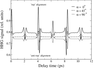
Figure 3: Calculated $19$th harmonic dynamic signal for N₂ for various pump-probe polarization angles, i.e. $\alpha=0^{o}$, $\alpha=45^{o}$, and $\alpha=90^{o}$; pump intensity $I=0.8\times 10^{14}$W/cm², probe intensity, $I=1.7\times 10^{14}$ W/cm², duration $40\,\mathrm{fs}$, and wavelength $800\,\mathrm{nm}$; Boltzmann temperature 200 K.

In Fig. 3 we show the results of computations using Eq. (8) for the dynamic signals from N₂ as a function of the delay time $t_{d}$, at three different relative polarization angles, $\alpha=$0${}^{o},\,45^{o}$, and $90^{o}$. The results show the full revival with a period $T_{rev}\equiv\frac{1}{2Bc}=8.4\,\mathrm{ps}$, and the fractional $\frac{1}{2}$ and $\frac{1}{4}$ revivals, for all three $\alpha$ values. The $\left\langle\left\langle\cos^{2}\theta\right\rangle\right\rangle\left(t_{d}\right)$ term is known to govern the $\frac{1}{2}$ and $\frac{1}{4}$ revivals and the associated Raman allowed spectral lines (e.g.exp_the ; fai_rou-01 ). Remarkably, the signals for $\alpha=$0^o and $\alpha=90^{o}$ are found to be in opposite phase, while that for $\alpha=0^{o}$ and $\alpha=45^{o}$ are in the same phase. Exactly the same phase relation between the $\alpha$-dependence of the $t_{d}$-signal from $N_{2}$ has been observed in recent experiments (e.g. miy-01 ; kan-01 ; miy-02 ).

To analyze their origin, we consider the leading term of Eq. (8) for N₂, more explicitly. (Below, we omit the argument $\left(t_{d}\right)$ for the sake of brevity.) Noting that $\left\langle\cos^{2}\theta^{\prime}\right\rangle=\frac{1}{2}\sin^{2}\alpha+(\cos^{2}\alpha-\frac{1}{2}\sin^{2}\alpha)\left\langle\cos^{2}\theta\right\rangle$ we get:

$$S\left(t_{d};\alpha\right) \approx \left(p_{1}+p_{2}\frac{1}{2}\sin^{2}\alpha\right)+p_{2}\left(\cos^{2}\alpha-\frac{1}{2}\sin^{2}\alpha\right)$$ (10)

$$\times\left\langle\left\langle\cos^{2}\theta\right\rangle\right\rangle+\cdots$$

Therefore, for the parallel polarizations we have, $S\left(t_{d};0^{o}\right)\approx p_{1}+p_{2}\left\langle\left\langle\cos^{2}\theta\right\rangle\right\rangle$ and for the perpendicular polarization, $S\left(t_{d};90^{o}\right)\approx\left(p_{1}+\frac{1}{2}p_{2}\right)-\frac{1}{2}p_{2}\left\langle\left\langle\cos^{2}\theta\right\rangle\right\rangle$. Clearly due to the opposite sign of the $\left\langle\left\langle\cos^{2}\theta\right\rangle\right\rangle$ term, they vary in opposite phase to each other from their respective bases. In contrast, the signal at $\alpha=45^{o}$, $S\left(t_{d},45^{o}\right)\approx\left(p_{1}+\frac{1}{4}p_{2}\right)+\frac{1}{4}p_{2}\left\langle\left\langle\cos^{2}\theta\right\rangle\right\rangle$, has the same sign of the $\left\langle\left\langle\cos^{2}\theta\right\rangle\right\rangle$ term as for $\alpha=$0, which makes them to vary in phase. These behaviors are what can be seen in the full calculations in Fig. 3, and they also agree with the recent experimental observations (e.g. ita-02 ; miy-01 ; kan-01 ; miy-02 ). The simple formula (10) predicts further that the extrema of the signal should occur for $\sin\alpha\cos\alpha=0$, with a maximum at $\alpha=$0^o and a minimum at $\alpha=90^{o}$. This is also what has been seen experimentally ita-02 ; miy-02 . Finally, (10) predicts a “magic angle” $\alpha_{c}=\arcsin\sqrt{\frac{2}{3}}\approx 54.7^{o}$, given by the condition $(\cos^{2}\alpha_{c}-\frac{1}{2}\sin^{2}\alpha_{c})=0$ at which the HHG signals become essentially independent of the delay $t_{d}$ between the pulses. Exactly such a “magic” crossing angle for N₂ signals has been observed experimentally miy-02 . We may point out that this geometry can be used in femtosecond pulse-probe experiments to generate an essentially steady HHG signal from freely rotating N₂.

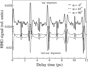
Figure 4: Calculated $19th$ HHG spectrum of O₂ for various pump-probe polarizations angle, i.e. $\alpha=0^{o}$, $\alpha=45^{o}$, and $\alpha=90^{o}$; pump intensity $I=0.5\times 10^{14}$W/cm², probe intensity, $I=1.2\times 10^{14}$ W/cm², duration $40\,\mathrm{fs}$, and wavelength $800\,\mathrm{nm}$; Boltzmann temperature 200 K.

In Fig. 4 we present the results of full calculations for O₂, using Eq. (9), for the three geometries, $\alpha=0^{o},\,45^{o}$, and $90^{o}$. The signals are seen to be characterized by a full revival at $T_{rev}=\frac{1}{2Bc}=11.6\,\mathrm{ps}$ and also by the fractional $\frac{1}{2}$ and $\frac{1}{4}$ revivals, like in N₂, as well as an additional $\frac{1}{8}$-revival, for all the three geometries; the same characteristics have been observed experimentally (e.g. kan-01 ; miy-02 ). The existence of the $\frac{1}{8}$-revival is due mainly to the presence of higher powers and moments than $\left\langle\left\langle\cos^{2}\theta\right\rangle\right\rangle$, that couple the Raman-forbidden ($\Delta J=\pm 4$) and the “anomalous” transitions ($|\Delta J|>4$) between the rotational states fai_rou-01 . We may express the contribution from the first term of Eq. (9) more explicitly as:

$$S\left(t_{d};\alpha\right) \approx \frac{q_{1}}{64}\left\langle\left\{\left(3-30\cos^{2}\alpha+35\cos^{4}\alpha\right)\right.\vphantom{\left\{\left(30\cos^{2}\alpha\right)\right.^{2}}\right.$$ (11)

$$\times\left\langle\sin^{2}\theta\cos^{2}\theta\right\rangle$$

$$-\left(1-6\cos^{2}\alpha+5\cos^{4}\alpha\right)\left\langle\cos^{2}\theta\right\rangle$$

$$+\left.\left.\left(4\sin^{2}\alpha-3\sin^{4}\alpha\right)\right\}^{2}\right\rangle+\cdots.$$

For $\alpha=0^{o}$, this gives, $S\left(t_{d};\alpha\right)\approx q_{1}\left\langle\left\langle\sin^{2}\theta\cos^{2}\theta\right\rangle^{2}\right\rangle$ and, for $\alpha=90^{o}$, $S\left(t_{d};\alpha\right)\approx q_{1}(\frac{3}{8})^{2}\left\langle\left\{\left\langle\sin^{2}\theta\cos^{2}\theta\right\rangle-\frac{1}{3}\left\langle\cos^{2}\theta\right\rangle+\frac{1}{3}\right\}^{2}\right\rangle$. A comparison of the above expressions suggests that for $\alpha=0^{o}$ and 90^o, the signals at the full, $\frac{1}{2}$ and $\frac{1}{4}$ revivals would be in opposite phase, and that at the $\frac{1}{8}$ revival would be in phase. A direct comparison of the calculations using the above abbreviated formulas with the full calculation in Fig. 4 and the experimental observations in O₂ (e.g. kan-01 ; miy-02 ), fully confirm the above expectations.

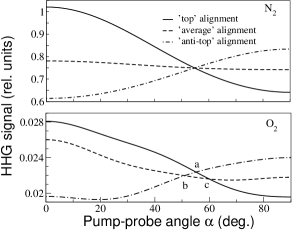
Figure 5: Variation of dynamic HHG signal as a function of pump-probe angle $\alpha$, near the first half-revival, for $N_{2}$ and $O_{2}$. The pulse parameters are the same as in Fig. (3) for $N_{2}$ and Fig. (4) for $O_{2}$.

In Fig. 5 we show the calculated results of the dynamical signals for N₂ (upper panel) and O₂ (lower panel), as a continuous function of $\alpha$, between 0^o to 90^o, at three different delay-times $t_{d}$ near the $\frac{1}{2}$ revival period. In the upper panel for N₂, a remarkable coincidence of the three signals is seen to occur at the “magic angle” $\alpha_{c}=\arcsin\sqrt{\frac{2}{3}}\approx 54.7^{o}$ as predicted above. Moreover, the signal at the “top”-alignment time $t_{d}=4.05\,\mathrm{ps}$ (solid curve) is seen to lie above the signal at the “anti-top” alignment time $t_{d}=4.3\,\mathrm{ps}$ (dash-dot curve), for all $\alpha<\alpha_{c}$, and they invert their relative strengths for all $\alpha>\alpha_{c}$. This is again in agreement with the recent observations (e.g. ita-02 ; miy-01 ). The corresponding signals for O₂ (lower panel) does not show a single crossing point, rather they cross at three different points a, b, and c in the neighborhood of the magic angle $\alpha_{c}\approx 54.7^{o}$. Such a crossover-neighborhood around the magic angle $\approx 54.7^{o}$ for O₂ is recently confirmed experimentally miy-02 . The absence of a single crossing point for O₂ is due mainly to the non-negligible contribution of the moment $\left\langle\left\langle\cos^{4}\theta\right\rangle\right\rangle$ to the O₂ signal (cf. Eq. (11)).

Before concluding, we may make a few qualitative remarks on the $\alpha$ dependence of the dynamic signals for the more complex triatomic molecule CO₂ miy-02 , and the organic molecule acetylene ($\pi$ symmetry), that are mesured recently kaj-02 ; tor-01 . The structure of the operator (7) shows, even without a detailed calculation, that the CO₂ and acetylene (HC$\equiv$CH), due to their linear structure, would show a similar crossover at or near $\alpha_{c}\approx 54.7^{o}$. A direct perusal of the experimental data miy-02 ; kaj-02 confirms this general expectation from the present theory – both CO₂ and acetylene exhibit the crossover effect, and indeed near the “magic angle” $\alpha_{c}=\arcsin\sqrt{\frac{2}{3}}\approx 54.7^{o}$.

To summarize: The simultaneous dependence of the dynamic HHG signals from coherently rotating linear molecules, on the relative polarization angle, $\alpha$, and the time delay, $t_{d}$, between a pump and a probe pulse, is investigated theoretically. A general formula for the dynamic signals for linear molecules is derived (Eqs. (6) and (7)). It is used to analyze the recently observed characteristics of the HHG signals from N₂ and O₂. Among other things, a “magic angle” $\alpha_{c}=\arcsin\sqrt{\frac{2}{3}}\approx 54.7^{o}$ for the crossing of the dynamic signals for N₂, and a crossover-neighborhood around the “magic angle”, for O₂, are predicted by the theory and confirmed by the available experimental data. The presence of analogous crossovers for the more complex linear molecules, CO₂, HC$\equiv$CH (acetylene), are also suggested by the present theory, and are corroborated by the recent observations.

References

(1) F. Rosca-Pruna and M.J.J. Vrakking, Phys. Rev.
Lett. 87, 153902 (2001); R. Velotta et al., Phys. Rev. Lett.
87, 183901 (2001); N. Hay et al., Phys. Rev. A 65,
053805 (2002); N. Hay et al., J. Mod. Opt. 50, 561 (2003);
P.W. Dooley et al., Phys. Rev. A 68, 023406 (2003); M. Lein
et al., Phys. Rev. A 67, 023819) (2003); J. Itatani et al.,
Nature 432, 867 (2004); R. de Nalda et al., Phys. Rev. A
69, 031804 (2004); M. Kaku et al., Japan J. Appl. Phys. 43,
L591 (2004). Zeidler et al. in Ultrafast Optics, IV, ed. F. Krauz
et al.,(Springer, New York, 2004); M. Lein et al., J. Mod. Opt. 52,
465 (2005); C. Vozzi et al., Phys. Rev. Lett, 95, 153902
(2005); X.X. Zhou et al., Phys. Rev. A 72, 033412 (2005);
C.B. Madsen and L.B. Madsen, Phys. Rev. A 74,023403(2006).
C. Vozzi et al., J.Phys. B. 39, S457 (2006).
(2) J. Itatani et al., Phys. Rev. Lett. 94,
123902 (2005).
(3) K. Miyazaki et al., Phys. Rev. Lett. 95,
243903 (2005).
(4) T. Kanai et al., Nature 435, 470 (2005).
(5) K. Miyazaki et al., IEEE-CLEO-PR-2007 Conf. Rep.
(submitted, 2007).
(6) N. Kajumba et al., Central Laser Facility
Ann. Rep., 2005/2006, p. 80, Rutherford Appleton Lab. U.K. (2006).
(7) R. Torres et al., Phys. Rev. Lett., 98,
203007 (2007).
(8) F.H.M. Faisal, A. Abdurrouf, G. Miyaji, and
K. Miyazaki, Phys. Rev. Lett., 98, 143001 (2007).
(9) A. Abdurrouf and F.H.M. Faisal, Phys. Rev. A
(to be submitted, 2007).
(10) H. Stapelfeldt and T. Seideman, Rev. Mod. Phys.
75, 543 (2003).
(11) A. Becker and F.H.M. Faisal, J. Phys. B 38,
R1 (2005).
(12) G. Herzberg, Molecular Spectra and Molecular
Structure, II (Van Nostard Reinhold, New York, (1950).