Multiphoton antiresonance in large-spin systems
Abstract
We study nonlinear response of a spin with easy-axis anisotropy. The response displays sharp dips or peaks when the modulation frequency is adiabatically swept through multiphoton resonance. The effect is a consequence of a special symmetry of the spin dynamics in a magnetic field for the anisotropy energy . The occurrence of the dips or peaks is determined by the spin state. Their shape strongly depends on the modulation amplitude. Higher-order anisotropy breaks the symmetry, leading to sharp steps in the response as function of frequency. The results bear on the dynamics of molecular magnets in a static magnetic field.
pacs:
75.50.Xx, 76.20.+q, 03.65.Sq, 75.45.+jI Introduction
Large-spin systems have been attracting much attention recently. Examples are and Mn impurities in semiconductors and Mn- and Fe-based molecular magnets with electron spin and higher. Nuclear spins have been also studied, and radiation-induced quantum coherence between the spin levels was observed Yusa et al. (2005). An important feature of large-spin systems is that their energy levels may be almost equidistant. A familiar example is spins in a strong magnetic field in the case of a relatively small magnetic anisotropy, where the interlevel distance is determined primarily by the Larmor frequency. Another example is low-lying levels of large- molecular magnets for small tunneling. As a consequence of the structure of the energy spectrum, external modulation can be close to resonance with many transitions at a time. This should lead to coherent nonlinear resonant effects that have no analog in two-level systems.
The effects of a strong resonant field on systems with nearly equidistant energy levels have been studied for weakly nonlinear oscillators. These studies concern both coherent effects, which occur without dissipation Larsen and Bloembergen (1976); Sazonov and Finkelstein (1976); Dmitriev and Dyakonov (1986), and incoherent effects, in particular those related to the oscillator bistability and transitions between coexisting stable states of forced vibrations. In the absence of dissipation, a nonlinear oscillator may display multiphoton antiresonance in which the susceptibility displays a dip or a peak as a function of modulation frequency Dykman and Fistul (2005).
In the present paper we study resonantly modulated spin systems with . Of primary interest are systems with uniaxial magnetic anisotropy, with the leading term in the anisotropy energy of the form of . We show that the coherent response of such spin systems displays peaks or dips when the modulation frequency adiabatically passes through multiphoton resonances. The effect is nonperturbative in the field amplitude. It is related to the special conformal property of the spin dynamics in the semiclassical limit. It should be noted that the occurrence of antiresonance for a spin does not follow from the results for the oscillator. A spin can be mapped onto a system of two oscillators rather than one; the transition matrix elements for a spin and an oscillator are different as are also the energy spectra.
We show that the coherent response of a spin is sensitive to terms of higher order in in the anisotropy energy. In addition, there is a close relation between the problem of resonant high-frequency response of a spin and the problem of static spin polarization transverse to the easy axis. Spin dynamics in a static magnetic field has been extensively studied both theoretically and experimentally Chudnovsky and Gunther (1988); Garanin (1991); Garg (1993); Friedman et al. (1996, 1997); Garanin and Chudnovsky (1997); Wernsdorfer and Sessoli (1999); Garg (1999); Villain and Fort (2000); Wernsdorfer et al. (2006). One of the puzzling observations on magnetization switching in molecular magnets, which remained unexplained except for the low-order perturbation theory, is that the longitudinal magnetic field at which the switching occurs is independent of the transverse magnetic field Friedman et al. (1997). The analysis presented below provides an explanation which is nonperturbative in the transverse field and also predicts the occurrence of peaks or dips in the static polarization transverse to the easy axis as the longitudinal magnetic field is swept through resonance.
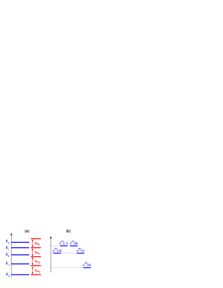
The onset of strong nonlinearity of the response due to near equidistance of the energy levels can be inferred from Fig. 1(a). It presents a sketch of the Zeeman levels of a spin () in a strong magnetic field along the easy magnetization axis . The spin Hamiltonian is
| (1) |
where is the Larmor frequency. For comparatively weak anisotropy, , the interlevel distances are close to each other and change linearly with .
A transverse periodic field leads to transitions between neighboring levels. An interesting situation occurs if the field frequency is close to and there is multiphoton resonance in the th state: coincides with the energy difference , . The amplitude of the resonant -photon transition in this case is comparatively large, because the transition goes via sequential one-photon virtual transitions which are all almost resonant. Therefore one should expect a comparatively strong multiphoton Rabi splitting already for a moderately strong field.
A far less obvious effect occurs in the coherent response of the system, that is in the magnetization at the modulation frequency or, equivalently, the susceptibility. As we show, the expectation value of the susceptibility displays sharp spikes at multiphoton resonance. The shape of the spikes very strongly depends on the field amplitude.
The paper is organized as follows. In Sec. II we study the quasienergy spectrum and the response of a spin with quadratic in anisotropy energy. We show that, at multiphoton resonance, not only multiple quasienergy levels are crossing pairwise, but the susceptibilities in the resonating states are also crossing. In Sec. III we show that multiphoton transitions, along with level repulsion, lead to the onset of spikes in the susceptibility and find the shape and amplitude of the spikes as functions of frequency and amplitude of the resonant field. In Sec. IV we present a WKB analysis of spin dynamics, which explains the simultaneous crossing of quasienergy levels and the susceptibilities beyond perturbation theory in the field amplitude. In Sec. V the role of terms of higher order in in the anisotropy energy is considered. Section VI contains concluding remarks.
II Low-field susceptibility crossing
II.1 The quasienergy spectrum
We first consider a spin with Hamiltonian (1), which is additionally modulated by an almost resonant ac field. The modulation can be described by adding to the term , where characterizes the amplitude of the ac field. As mentioned above, we assume that the field frequency is close to and that .
It is convenient to describe the modulated system in the quasienergy, or Floquet representation. The Floquet eigenstates have the property , where is the modulation period and is quasienergy. For resonant modulation, quasienergy states can be found by changing to the rotating frame using the canonical transformation . In the rotating wave approximation the transformed Hamiltonian is
| (2) | |||
Here we disregarded fast-oscillating terms .
The Hamiltonian has a familiar form of the Hamiltonian of a spin in a scaled static magnetic field with components and along the and axes, respectively. Much theoretical work has been done on spin dynamics described by this Hamiltonian in the context of molecular magnets.
The eigenvalues of give quasienergies of the modulated spin. In the weak modulating field limit, , the quasienergies are shown in Fig.1(b). In this limit spin states are the Zeeman states, i.e., the eigenstates of , with . The interesting feature of the spectrum, which is characteristic of the magnetic anisotropy of the form , is that several states become simultaneously degenerate pairwise for Friedman et al. (1997); Garanin and Chudnovsky (1997). From Eq. (2), the quasienergies and are degenerate if the modulation frequency is
| (3) |
The condition (3) is simultaneously met for all pairs of states with given . It coincides with the condition of -photon resonance . In what follows can be positive and negative. There are frequency values that satisfy the condition (3) for a given .
The field leads to transitions between the states and to quasienergy splitting. The level splitting for the Hamiltonian (2) was calculated earlier Garanin and Chudnovsky (1997). For multiphoton resonance, it is equal to twice the multiphoton Rabi frequency ,
| (4) |
The -photon Rabi frequency (II.1) is , as expected. We note that the amplitude is scaled by the anisotropy parameter , which characterizes the nonequidistance of the energy levels and is much smaller than the Larmor frequency. Therefore becomes comparatively large already for moderately weak fields .
We denote the true quasienergy states as , with integer or half-integer such that . The quasienergies do not cross. One can enumerate the states by thinking of them as the adiabatic states for slowly increasing , starting from large negative . For the states are very close to the Zeeman states , with being the eigenvalue of . This then specifies the values of for all .
If the field is weak, the states are close to the corresponding Zeeman states, , for all except for narrow vicinities of the resonant values given by Eq. (3). The relation between the numbers and for is
| (5) |
where runs from to ; the term is eliminated, which is indicated by the prime over the sum; is the step function. In obtaining Eq. (5) we took into account that, for weak fields, only neighboring quasienergy levels and come close to each other. Eq. 5) defines the state enumerating function .
The enumeration scheme and the avoided crossing of the quasienergy levels are illustrated in Fig. 2. For the chosen the anticrossing occurs for 7 frequency values, as follows from Eq. (3). The magnitude of the splitting strongly depends on : the largest splitting occurs for one-photon transitions. It is also obvious from Fig. 2 that several levels experience anticrossing for the same modulation frequency.
II.2 Susceptibility and quasienergy crossing
Of central interest to us it the nonlinear susceptibility of the spin. We define the dimensionless susceptibility in the quasienergy state as the ratio of the expectation value of the appropriately scaled magnetization at the modulation frequency to the modulation amplitude,
| (6) |
In the weak field limit, .
| (7) |
where and are related by Eq. (5); in fact, Eq. (7) gives the susceptibility in the perturbed to first order in Zeeman state .
A remarkable feature of Eq. (7) is the susceptibility crossing at multiphoton resonance. The susceptibilities in Zeeman states and are equal where the unperturbed quasienergies of these states are equal, , i.e., where the frequency detuning is . In terms of the adiabatic states , for such we have from Eqs. (5), (7) for .
A direct calculation shows that simultaneous crossing of the susceptibilities and quasienergies occurs also in the fourth order of the perturbation theory provided . Numerical diagonalization of the Hamiltonian (2) indicates that it persists in higher orders, too, until level repulsion due to multiphoton Rabi oscillations comes into play.
The susceptibility is immediately related to the field dependence of the quasienergy . Since , from the explicit form of the Hamiltonian (2) we have
| (8) |
Simultaneous crossing of the susceptibilities and quasienergies means that, for an -photon resonance, the Stark shift of resonating states is the same up to order in ; only in the th order the levels and become split [by ]. Respectively, the susceptibilities and coincide up to terms . The physical mechanism of this special behavior is related to the conformal property of the spin dynamics, as explained in Sec. IV.
Equation (7) does not apply in the case of one-photon resonance, : it gives for . This is similar to the case of one-photon resonance in a two-level system, where the behavior of the susceptibility is well understood beyond perturbation theory. Interestingly, the lowest-order perturbation theory does not apply also at exact two-photon resonance, , as discussed below, even though Eq. (7) does not diverge.
III Antiresonance of the multiphoton response
The field-induced anticrossing of quasienergy levels at multiphoton resonance is accompanied by lifting the degeneracy of the susceptibilities. It leads to the onset of a resonant peak and an antiresonant dip in the susceptibilities as functions of frequency . The behavior of the quasienergy levels and the susceptibilities is seen from Fig. 3. For small field amplitude the multiphoton Rabi frequency is small, the quasienergies of interest and (with ) come very close to each other at resonant , as do also the susceptibilities and .
With increasing the level splitting rapidly increases in a standard way. The behavior of the susceptibilities is more complicated. They cross, but sufficiently close to resonance they repel each other, forming narrow dips (antiresonance) or peaks (resonance). The widths and amplitudes of the dips/peaks display a sharp dependence on the amplitude and frequency of the field.
For weak field it is straightforward to find the splitting of the susceptibilities
close to -photon resonance between states and . In this region the frequency detuning from the resonance
| (9) |
is small, . To the lowest order in but for an arbitrary ratio the quasienergy states and are linear combinations of the states and . Then from Eq. (2) it follows that the splitting of the quasienergies is
| (10) |
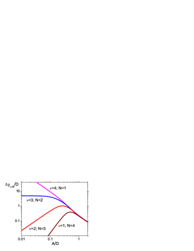
The splitting as a function of frequency is maximal at -photon resonance, . The half-width of the peak of at half height is determined by the Rabi splitting and is equal to . The peak is strongly non-Lorentzian, it is sharper than the Lorentzian curve with the same half-width. This sharpness is indeed seen in Fig. 3. Our numerical results show that Eq. (11) well describes the splitting in the whole frequency range .
For small , the susceptibility splitting is stronger than the level repulsion. It follows from Eqs. (10), (11) that at exact -photon resonance whereas . This scaling is seen in Fig. 4. For , on the other hand, the eigenstates become close to the eigenstates of a spin with Hamiltonian . As a result, the susceptibility splitting decreases with increasing , ; the proportionality coefficient here is independent of . Therefore, for displays a maximum as a function of , as seen from Fig. 4.
III.1 Two-photon resonance
As mentioned above, the lowest order perturbation theory (7) does not describe resonant susceptibility for two-photon resonance. Indeed, it follows from Eq. (11) that at exact resonance, , the susceptibility splitting for weak fields is
| (12) | |||||
This splitting is independent of . The expression for the susceptibility (7) is also independent of , yet it does not lead to susceptibility splitting and therefore is incorrect at two-photon resonance.
The inapplicability of the simple perturbation theory (7) is a consequence of quantum interference of transitions, the effect known in the linear response of multilevel systems Dykman and Krivoglaz (1984). To the leading order in , the susceptibility is determined by the squared amplitudes of virtual transitions to neighboring states. For a two-photon resonance, , the distances between the levels involved in the transitions and are equal, . Therefore the transitions resonate and interfere with each other.
To calculate the susceptibility it is necessary to start with a superposition of states and , add the appropriately weighted amplitudes of transitions and , and then square the result. This gives the correct answer. The independence of the susceptibility splitting from for two-photon resonance in the range of small as given by Eq. (12) is seen in Fig. 4.
IV Susceptibility crossing for a semiclassical spin
The analysis of the simultaneous level and susceptibility crossing is particularly interesting and revealing for large spins and for multiphoton transitions with large . For the spin dynamics can be described in the WKB approximation. We will start with the classical limit. In this limit it is convenient to use a unit vector , with , where and are the polar and azimuthal angles of the vector . To the lowest order in equations of motion for the spin components can be written as
| (13) | |||
Here, overdot implies differentiation with respect to dimensionless time , that is, . Equations (13) preserve the length of the vector and also the reduced Hamiltonian ,
| (14) |
For convenience, we added to the term .
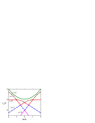
The effective energy is shown in Fig. 5. Also shown in this figure are the positions of the stationary states and examples of the phase trajectories described by Eqs. (13).
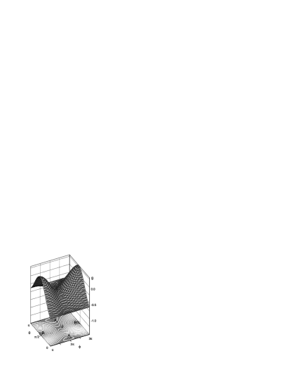
An insight into the spin dynamics can be gained by noticing that has the form of the scaled free energy of an easy axis ferromagnet Landau and Lifshitz (2004), with playing the role of the magnetization , and with and being the reduced components of the magnetic field along the easy axis and the transverse axis , respectively. In the region
| (15) |
the function has two minima, and , a maximum , and a saddle point . We will assume that the minimum is deeper than , that is
| (16) |
As seen from Eqs. (13) and (14) and Fig. 5, for the minima and the saddle point are located at and the maximum is at ; the case corresponds to a replacement . On the boundary of the hysteresis region (15) the shallower minimum merges with the saddle point .
In the case of an easy-axis ferromagnet with free energy , the minima of correspond to coexisting states of magnetization within the hysteresis region (15). For multiphoton absorption is the scaled quasienergy, not free energy, and stability is determined dynamically by balance between relaxation and high-frequency excitation. One can show that, for relevant energy relaxation mechanisms, the system can have coexisting stable stationary states inside and outside the region (15). The states correspond to one or both minima and/or the maximum of ; for small damping the actual stable states are slightly shifted away from the extrema of on the ()-plane. We will not discuss relaxation effects in this paper.
IV.1 Conformal property of classical trajectories
Dynamical trajectories of a classical spin on the plane are the lines const. They are either closed orbits around one of the minima or the maximum of , or open orbits along the axis, see Fig. 5. On the Bloch sphere , closed orbits correspond to precession of the unit vector around the points , or , in which does not make a complete turn around the polar axis. Open orbits correspond to spinning of around the polar axis accompanied by oscillations of the polar angle . Even though the spin has 3 components, the spin dynamics is the dynamics with one degree of freedom, the orbits on the Bloch sphere do not cross.
An important feature of the dynamics of a classical spin in the hysteresis region is that, for each in the interval , the spin has two coexisting orbits, see Fig. 5. One of them corresponds to spin precession around . It can be a closed loop or an open trajectory around the point on the -plane. The other is an open trajectory on the opposite side of the -surface with respect to the saddle point. We will classify them as orbits of type I and II, respectively.
We show in Appendix that classical equations of motion can be solved in an explicit form, and the time dependence is described by the Jacobi elliptic functions. The solution has special symmetry. It is related to the conformal property of the mapping of onto . The major results of the analysis are the following features of the trajectories of types I and II: for equal , (i) their dimensionless oscillation frequencies are equal to each other, and (ii) the period averaged values of the component are equal, too,
| (17) |
Here, the subscripts I and II indicate the trajectory type. The angular brackets imply period averaging on a trajectory with a given .
The quantity gives the classical response of the spin to the field . Equation (17) shows that this response is equal for the trajectories with equal values of the effective Hamiltonian function . This result holds for any field amplitude , it is by no means limited to small where the perturbation theory in applies.
IV.2 The WKB picture in the neglect of tunneling
In the WKB approximation, the values of quasienergy in the neglect of tunneling can be found by quantizing classical orbits const, see Ref. Garg and Stone, 2004 and papers cited therein. Such quantization should be done both for orbits of type I and type II, and we classify the resulting states as the states of type I and II, respectively. The distance between the states of the same type in energy units is Landau and Lifshitz (1981). Transitions between states of types I and II with the same are due to tunneling.
If we disregard tunneling, the quasienergy levels of states I and II will cross, for certain values of . Remarkably, if two levels cross for a given , then all levels in the range cross pairwise. This is due to the fact that the frequencies and thus the interlevel distances for the two sets of states are the same, see Eq. (17). Such simultaneous degeneracy of multiple pairs of levels agrees with the result of the low-order quantum perturbation theory in and with numerical calculations.
In the WKB approximation, the expectation value of an operator in a quantum state is equal to the period-averaged value of the corresponding classical quantity along the appropriate classical orbit Landau and Lifshitz (1981). Therefore if semiclassical states of type I and II have the same , the expectation values of the operator in these states are the same according to Eq. (17). Thus, the WKB theory predicts that, in the neglect of tunneling, there occurs simultaneous crossing of quasienergy levels and susceptibilities for all pairs of states with quasienergies between and . This is in agreement with the result of the perturbation theory in and with numerical calculations. However, we emphasize that the WKB theory is not limited to small , and the WKB analysis reveals the symmetry leading to the simultaneous crossing of quasienergy levels and the susceptibilities.
Tunneling between semiclassical states with equal leads to level repulsion and susceptibility antiresonance. The level splitting can be calculated by appropriately generalizing the standard WKB technique, for example as it was done in the analysis of tunneling between quasienergy states of a modulated oscillator Dmitriev and Dyakonov (1986). Then the resonant susceptibility splitting can be found from Eq. (8). The corresponding calculation is beyond the scope of this paper.
V Degeneracy lifting by higher order terms in
The simultaneous crossing of quasienergy levels and susceptibilities in the neglect of tunneling is a feature of the spin dynamics described by Hamiltonian (2). Higher-order terms in lift both this degeneracy and the property that many quasienergy levels are pairwise degenerate for the same values of the frequency detuning . The effect is seen already if we incorporate the term in the anisotropy energy, i.e. for a spin with Hamiltonian
| (18) |
The Hamiltonian is written in the rotating wave approximation, is given by Eq. (2), and is the parameter of quartic anisotropy. The terms in the spin anisotropy energy do not show up in even if they are present in the spin Hamiltonian but the corresponding anisotropy parameters are small compared to . In the rotating frame these terms renormalize the coefficient at and lead to fast oscillating terms that we disregard.
Multiple pairwise degeneracy occurs where the condition on Zeeman quasienergies is simultaneously met for several pairs . For this happens only for , that is when the modulation frequency is equal to the Larmor frequency . In this case the resonating Zeeman states are and with the same . The susceptibilities of these states are equal by symmetry with respect to reflection in the plane .
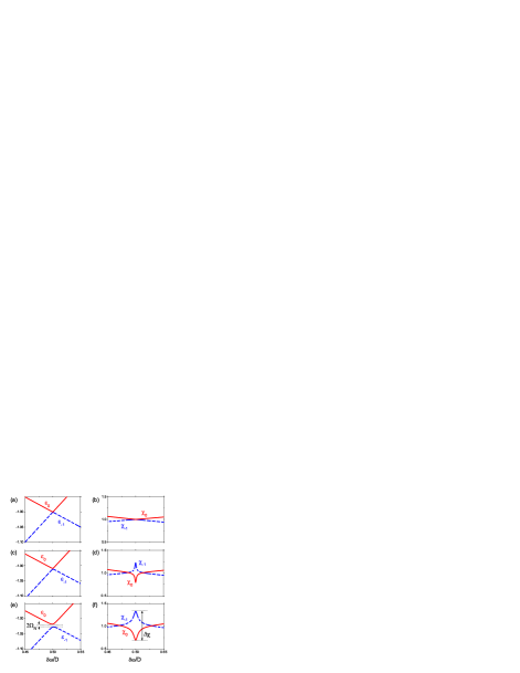
-photon resonance for nonzero and occurs generally only for one pair of states and . This is seen from panel (a) in Fig. 6. With increasing the difference in the resonant values of frequency increases, as seen from panel (c) in the same figure.
The susceptibilities in resonating states are different in the weak-field limit. When the frequency adiabatically goes through resonance, there occurs an interchange of states, for weak field : if the state was close to on one side of resonance, it becomes close to on the other side. Respectively, the susceptibility sharply switches from its value in the state to its value in the state .
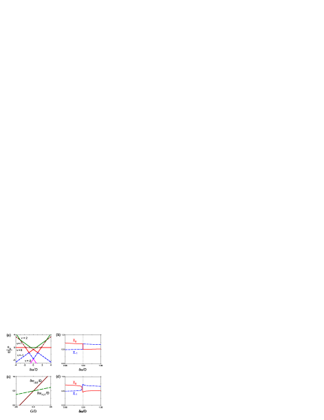
Susceptibility switching is seen in panels (b) and (d) in Fig. 6. For a weak field the frequency range where the switching occurs is narrow and the switching is sharp (vertical, in the limit ). As the modulation amplitude increases the range of frequency detuning over which the switching occurs broadens. In addition, for small the susceptibility displays spikes. They have the same nature as for . However, they are much less pronounced, as seen from the comparison of panel (d) in Fig. 6 and panel (f) in Fig. 3 which refer to the same value of .
VI Conclusions
In this paper we have considered a large spin with an easy axis anisotropy. The spin is in a strong magnetic field along the easy axis and is additionally modulated by a transverse field with frequency close to the Larmor frequency . We have studied the coherent resonant response of the spin. It is determined by the expectation value of the spin component transverse to the easy axis. We are interested in multiphoton resonance where coincides or is very close to the difference of the Zeeman energies in the absence of modulation.
The major results refer to the case where the anisotropy energy is of the form . In this case not only the quasienergies of the resonating Zeeman states and cross at multiphoton resonance, but the susceptibilities in these states also cross, in the weak-modulation limit. Such crossing occurs simultaneously for several pairs of Zeeman states. As the modulation amplitude increases, the levels are Stark-shifted and the susceptibilities are also changed. However, as long as the Rabi splitting due to resonant multiphoton transitions (tunneling) can be disregarded, for resonant frequency the quasienergy levels remain pairwise degenerate and the susceptibilities remain crossing. We show that this effect is nonperturbative in , it is due to the special conformal property of the classical spin dynamics.
Resonant multiphoton transitions lift the degeneracy of quasienergy levels, leading to a standard level anticrossing. In contrast, the susceptibilities as functions of frequency cross each other. However, near resonance they display spikes. The spikes of the involved susceptibilities point in the opposite direction, leading to decrease (antiresonance) or increase (resonance) of the response. They have a profoundly non-Lorentzian shape (11), with width and height that strongly depend on . The spikes can be observed by adiabatically sweeping the modulation frequency through a multiphoton resonance. If the spin is initially in the ground state, a sequence of such sweeps allows one to study the susceptibility in any excited state provided the relaxation time is long enough.
The behavior of the susceptibilities changes if terms of higher order in in the anisotropy energy are substantial. In this case crossing of quasienergy levels is not accompanied by crossing of the susceptibilities in the limit . Resonant multiphoton transitions lead to step-like switching between the branches of the susceptibilities of the resonating Zeeman states. Still, the susceptibilities display spikes as functions of frequency for a sufficiently strong modulating field.
The results of the paper can be applied also to molecular magnets in a static magnetic field. The spin Hamiltonian in the rotating wave approximation (2) is similar to the Hamiltonian of a spin in a comparatively weak static field, with the Larmor frequency of the same order as the anisotropy parameter . The susceptibility then characterizes the response to the field component transverse to the easy axis. Quasienergies are now spin energies in the absence of the transverse field, and instead of multiphoton resonance we have resonant tunneling. Our results show that a transverse field does not change the value of the longitudinal field for which the energy levels cross, in the neglect of tunneling. This explains the experiment Friedman et al. (1997) where such behavior was observed.
In conclusion, we have studied multiphoton resonance in large-spin systems. We have shown that the coherent nonlinear response of the spin displays spikes when the modulation frequency goes through resonance. The spikes have non-Lorentzian shape which strongly depends on the modulation amplitude. The results bear on the dynamics of molecular magnets in a static magnetic field and provide an explanation of the experiment.
We acknowledge insightful discussions with B.L. Altshuler and A. Kamenev. This work was supported by the NSF through grants No. ITR-0085922 and PHY-0555346.
Appendix A Symmetry of classical spin dynamics: a feature of the conformal mapping
Classical equations of motion for the spin components (13) can be solved in the explicit form, taking into account that and that const on a classical trajectory. For time evolution of the -component of the spin we obtain
| (19) |
where are the roots of the equation
| (20) |
and is the Jacobi elliptic function. The argument and the parameter are
| (21) |
Equation (19) describes an orbit which, for a given , oscillates between and ; the corresponding oscillations of can be easily found from Eqs. (13), (14).
Oscillations of between and for the same are also described by Eq. (19) provided one replaces , where is the elliptic integral and . Clearly, both types of oscillations have the same period over equal to . They correspond, respectively, to the trajectories of types II and I in Fig. 5 that lie on different sides of -surface. As a consequence, the vibration frequencies for the corresponding trajectories and are the same. This proves the first relation in Eq. (17).
The Jacobi elliptic functions are double periodic, and therefore is also double periodic,
| (22) |
with integer . Ultimately, this is related to the fact that equations of motion (13) after simple transformations can be put into a form of a Schwartz-Christoffel integral that performs conformal mapping of the half-plane Im onto a rectangle on the -plane.

We will show now that the mapping has a special property that leads to equal period-averaged values of on trajectories of different types but with the same . Because is double periodic, cf. Eq. (22), so is also the function . Keeping in mind that the transformation moves us from a trajectory with a given of type I to a trajectory of type II, we can write the difference of the period-averaged values of on the two trajectories as
| (23) |
where the contour is a parallelogram on the -plane with vortices at . It is shown in Fig. 7.
An important property of the mapping (19) is that has one simple pole inside the contour , as marked in Fig. 7. Respectively, has a second-order pole. The explicit expression (19) allows one to find the corresponding residue. A somewhat cumbersome calculation shows that it is equal to zero. This shows that the period-averaged values of on the trajectories with the same coincide, thus proving the second relation in Eq. (17).
References
- Yusa et al. (2005) G. Yusa, K. Muraki, K. Takashina, K. Hashimoto, and Y. Hirayama, Nature 434, 1001 (2005).
- Larsen and Bloembergen (1976) D. M. Larsen and N. Bloembergen, Opt. Commun. 17, 254 (1976).
- Sazonov and Finkelstein (1976) V. N. Sazonov and V. I. Finkelstein, Doklady Akad. Nauk SSSR 231, 78 (1976).
- Dmitriev and Dyakonov (1986) A. P. Dmitriev and M. I. Dyakonov, Zh. Eksper. Teor. Fiz. 90, 1430 (1986).
- Dykman and Fistul (2005) M. I. Dykman and M. V. Fistul, Phys. Rev. B 71, 140508 (2005).
- Chudnovsky and Gunther (1988) E. M. Chudnovsky and L. Gunther, Phys. Rev. Lett. 60, 661 (1988).
- Garanin (1991) D. A. Garanin, J. Phys. A 24, L61 (1991).
- Garg (1993) A. Garg, Europhys. Lett. 22, 205 (1993).
- Friedman et al. (1996) J. R. Friedman, M. P. Sarachik, J. Tejada, and R. Ziolo, Phys. Rev. Lett. 76, 3830 (1996).
- Friedman et al. (1997) J. R. Friedman, M. P. Sarachik, J. M. Hernandez, X. X. Zhang, J. Tejada, E. Molins, and R. Ziolo, J. Appl. Phys. 81, 3978 (1997).
- Garanin and Chudnovsky (1997) D. A. Garanin and E. M. Chudnovsky, Phys. Rev. B 56, 11102 (1997).
- Wernsdorfer and Sessoli (1999) W. Wernsdorfer and R. Sessoli, Science 284, 133 (1999).
- Garg (1999) A. Garg, Phys. Rev. Lett. 83, 4385 (1999).
- Villain and Fort (2000) J. Villain and A. Fort, Eur. Phys. J. B 17, 69 (2000).
- Wernsdorfer et al. (2006) W. Wernsdorfer, M. Murugesu, and G. Christou, Phys. Rev. Lett. 96, 057208 (2006).
- Dykman and Krivoglaz (1984) M. I. Dykman and M. A. Krivoglaz, Soviet Physics Reviews (Harwood Academic, New York, 1984), vol. 5, pp. 265–441.
- Landau and Lifshitz (2004) L. D. Landau and E. M. Lifshitz, Electrodynamics of Continuous Media (Elsevier Butterworth-Heinemann, Oxford, 2004), 2nd ed.
- Garg and Stone (2004) A. Garg and M. Stone, Phys. Rev. Lett. 92, 010401 (2004).
- Landau and Lifshitz (1981) L. D. Landau and E. M. Lifshitz, Quantum mechanics. Non-relativistic theory (Butterworth-Heinemann, Oxford, 1981), 3rd ed.