Logarithmic corrections in the aging of the fully-frustrated Ising model

Abstract

We study the dynamics of the critical two-dimensional fully-frustrated Ising model by means of Monte Carlo simulations. The dynamical exponent is estimated at equilibrium and is shown to be compatible with the value $z_{c}=2$. In a second step, the system is prepared in the paramagnetic phase and then quenched at its critical temperature $T_{c}=0$. Numerical evidences for the existence of logarithmic corrections in the aging regime are presented. These corrections may be related to the topological defects observed in other fully-frustrated models. The autocorrelation exponent is estimated to be $\lambda=d$ as for the Ising chain quenched at $T_{c}=0$.

Introduction

Out-of-equilibrium statistical physics is a very active field of research. Among the most studied topics, the slow evolution of glasses remains a challenging problem. During a quench in the glass phase, the system is trapped in an infinite succession of metastable states and never reaches equilibrium. Time-translation invariance is broken and the fluctuation-dissipation theorem does not hold anymore [1, 2, 3]. Frustration and randomness are two key ingredients in the behavior of glasses. Interestingly, neither frustration nor randomness are necessary conditions for aging. Indeed it is known for a decade that homogeneous ferromagnets can also display aging. When they are prepared in their paramagnetic phase and then quenched below their critical temperature $T_{c}$ for example, ferromagnets age due to metastable states consisting in ferromagnetic domains in competition. The domain walls between them cannot be eliminated in a finite time [4]. The divergence of the relaxation time provokes the suppression of the exponential relaxation and two-time observables, for instance the autocorrelation function $C(t,s)$, decays as a power-law of the scaling variable $t/s$. A more detailed presentation will be given in section 3.

In this work, we are interested in the intermediate situation of frustrated systems but without disorder. The model considered is the critical two-dimensional fully-frustrated Ising model (FFIM). The equilibrium properties of the FFIM will be presented in section 1. The FFIM belongs to the same universality class as the anti-ferromagnetic Ising model on a triangular lattice (AFIT). As a consequence, one may assume that these two models display the same behavior out-of-equilibrium. This is indeed claimed in a note in Ref. [5]. However, controversial results are found in the literature about the AFIT. On the one hand, numerical evidences suggesting the existence of topological defects in anti-ferromagnetic Ising and Potts models have been given [6, 7]. Out-of-equilibrium, these topological defects behave as impurities and pin the domain walls. The motion of the latter is thus slowed down by a logarithmic factor which is then observable in dynamical quantities [4]. Such a mechanism is also encountered in pure systems where topological defects are present too. The paradigmatic model in this case is the two-dimensional XY model for which it has been shown that vortices manifest themselves by logarithmic corrections in the long-time behavior of the dynamical observables [4, 8]. Such logarithmic corrections have been observed [7] in the AFIT. Like in the XY model, the dynamical exponent is predicted to be $z_{c}=2$ in the AFIT since it exists an exact mapping onto a Gaussian Solid-on-Solid model [9]. On the other hand, a recent Monte Carlo simulation of the anti-ferromagnetic Ising model failed to observe such logarithmic corrections [5]. In contradistinction to the previous scenario, the dynamical exponent was estimated to be $z_{c}\simeq 2.33$. The spin-spin autocorrelation was observed to decay as a power-law with an exponent $\lambda_{c}/z_{c}\simeq 0.86$.

Our goal is to investigate the existence of logarithmic corrections in the FFIM. To that purpose, we will estimate the dynamical exponent $z_{c}$ at equilibrium in section 2. Remind that the two scenarii give quite different values. In section 3, we will study the aging properties and search for the signature of topological defects when the system is quenched from the paramagnetic phase. The ratio $\lambda/z$ will be estimated and compared to the different scenarii.

1 The Fully-Frustrated Ising Model (FFIM)

We consider the classical two-dimensional fully-frustrated Ising model (FFIM) defined by the Hamiltonian

$${\cal H}=-\sum_{x,y}\left[\sigma_{x,y}\sigma_{x+1,y}+(-1)^{f(x,y)}\sigma_{x,y}\sigma_{x,y+1}\right],\quad\sigma_{x,y}\in\{-1,1\}.$$ (1)

The function $f(x,y)$ is chosen such that each plaquette has an odd number of anti-ferromagnetic couplings. As a consequence there exists no spin configuration for which all bonds can be satisfied. The most studied coupling configurations correspond to $f(x,y)=x+y$ (Zig-Zag) and $f(x,y)=x$ (Piled-up Domino). They are depicted on Figure 1. At equilibrium, these two coupling configurations are equivalent since a transformation leaving the partition function unchanged maps one onto the other [10]. In this study, we will consider the Zig-Zag coupling configuration.

Figure 1: Coupling configurations discussed in the text: Zig-Zag (left) and Piled-up Domino (right) configurations. Thin lines correspond to ferromagnetic couplings and thick ones to anti-ferromagnetic couplings.

Spin configurations in the ground state can be obtained by minimization of the energy of each plaquette independently. Since by construction of the model it is not possible to satisfy all the bonds in a plaquette, the possible spin configurations in the ground state are those with only one unsatisfied bond. They are shown on Figure 2. The ground-state is then built by juxtaposition of these plaquettes. Even when three out of the four spins of the plaquette are fixed by neighboring plaquettes, there may exist several possibilities to choose the fourth spin (the two last plaquettes of Figure 2 give an example of such a situation). As a consequence, the ground state is highly degenerate and the entropy per site is finite at $T=0$ [11]. One can describe the spin configurations at $T=0$ as made of ferromagnetic domains separated by domain walls. The possible plaquettes in the ground state forbid that more than one domain wall goes through a plaquette which means that domain walls cannot intersect each other. Moreover, when going through a plaquette, the domain wall must cross the anti-ferromagnetic bond and one of the three ferromagnetic bonds. Figure 3 shows examples of spin configurations in the ground state. In the case of the Zig-Zag coupling configuration, domain walls cannot form overhangs or loops. They must start and end at two different boundaries of the system. For the Piled-up Domino coupling configuration, domain walls can form overhangs and loops. They can thus enclose finite clusters that can be as small as one single spin.

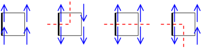
Figure 2: Possible spin configurations on a plaquette in the ground state. The dashed lines correspond to the domain walls between the different ferromagnetic phases.

The equilibrium properties of the FFIM have been determined by analytical diagonalization of the transfer matrix [12]. The ferromagnetic order is destroyed at any temperature because the domain walls discussed above have no energy. Nevertheless, the system is critical at $T_{c}=0$ with spin-spin correlation functions decaying algebraically with an exponent $\eta=1/2$ [13]. As already mentioned in the introduction, the FFIM belongs to the same universality class as the homogeneous anti-ferromagnetic Ising model on a triangular lattice [14] (AFIT).

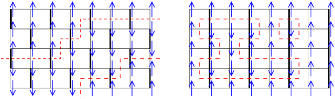
Figure 3: Examples of spin configurations in the ground state of the FFIM for the Zig-Zag (left) and the Piled-up Domino coupling configuration (right).

2 Dynamical exponent of the FFIM

We now consider the dynamical properties of the FFIM at equilibrium at its critical temperature $T_{c}=0$. The system is initially thermalized and then evolves with the Glauber dynamics [15]. For an inverse temperature $\beta=1/k_{B}T$, the probability for a spin to be flipped is ${e^{-\beta\Delta E}\over 1+e^{-\beta\Delta E}}$ where $\Delta E$ is the variation of energy when the spin is flipped. In our case, the temperature is $T=0$ which means that a spin flip is always accepted if the energy is lowered, accepted with a probability $1/2$ if the energy does not change, and always rejected otherwise. Moreover, we start from an equilibrium state at $T=0$, i.e. with the minimal value of the energy. As a consequence, the algorithm becomes particularly simple: a spin is randomly chosen and is flipped if the total energy does not change .

In contradistinction to homogeneous ferromagnets, the Glauber dynamics of the FFIM is not frozen at $T=0$. In the case of the Zig-Zag coupling configuration, some single-spin flips, as for instance the formation of a dot on a flat domain wall, does not change the total energy and are thus allowed. In the case of the Pile-up Domino coupling configuration, one can also flip any spin which lies on an anti-ferromagnetic bond in the bulk of a ferromagnetic domain. This process creates a new single-spin domain as the one depicted on Figure 3. These single-spin domains can be flipped without any energy change. As a consequence, they behave as isolated Ising spins. This situation was already encountered in the case of the AFIT where these spins were called loose spins [13].

The dynamical exponent $z_{c}$ of the FFIM at $T=0$ is not known. Since the FFIM belongs to the same universality class at equilibrium as the AFIT, one may assume that they share the same dynamical exponents $z_{c}$. As already mentioned in the introduction, different values can be found in the literature. According to Moore et al. [7] who claim the existence of topological defects, the dynamical exponent should be $z_{c}=2$. On the other hand, the numerical estimate $z_{c}\simeq 2.33$ has been determined in more recent Monte Carlo simulations [5].

To measure the critical exponent in the FFIM, we computed the spin-spin autocorrelation function at equilibrium at $T_{c}=0$. The lattice size is $192\times 192$ and we used periodic boundary conditions in both directions. The system is first thermalized using the Kandel-Ben Av-Domany cluster algorithm [16]. We then use the Glauber dynamics and measure $\sigma_{i}(s)$ and $\sigma_{i}(t)$. The simulation is repeated 1000 times. The mean spin-spin autocorrelation is finally estimated as

$$C_{\rm eq.}(t,s)={1\over N}\sum_{i}\langle\sigma_{i}(t)\sigma_{i}(s)\rangle$$ (2)

where $\langle\ldots\rangle$ denotes the average over the 1000 histories of the system. As shown on Figure 4, the correlation function decays as a power-law for sufficiently large separation time ($t-s>10$). One indeed expects that the divergence of the relaxation time at the critical point leads to an algebraic decay of the autocorrelation function $C(t,s)$. Moreover, time-translation invariance at equilibrium imposes a dependence on $t-s$. Finally, the order parameter having an anomalous dimension $\beta/\nu$, one expects

$$C_{\rm eq.}(t,s)\mathrel{\mathop{\kern 0.0pt\sim}\limits_{t-s\gg 1}}(t-s)^{-2\beta/\nu z_{c}}$$ (3)

The interpolation of the data (Figure 4) with this expression leads to the estimate $2\beta/\nu z_{c}=0.2495(11)$. Since $\eta=2\beta/\nu=1/2$ ($d=2$), our estimate for the dynamical exponent is $z_{c}\simeq 2.004(9)$. This value is compatible with $z_{c}=2$, i.e. the one expected in the scenario involving topological defects [7] and contradicts the observation of a sub-diffusive growth with $z\simeq 2.33$ observed by Kim et al. [5] with random initial configurations in the AFIT. Note that we also measured the dynamical exponent $z_{c}$ during a quench by considering the decay of autocorrelation functions in the quasi-equilibrium regime. We obtained again a value compatible with $z_{c}=2$.

Figure 4: Equilibrium spin-spin autocorrelation function $C(t,s)$ of the FFIM at $T_{c}=0$ with the Zig-Zag coupling configuration versus $t-s$. The six curves corresponding to $s=10,20,40,160,640$ and $s=1280$ cannot be distinguished as expected at equilibrium. A very nice power-law is observed and allows for a precise determination of $2\beta/\nu z_{c}$.

3 Aging of the FFIM

We are now interested in the out-of-equilibrium dynamics of the FFIM. The system is initially prepared at $T\rightarrow+\infty$, i.e. spins are random. It it then quenched at the critical temperature $T_{c}=0$. We use the Glauber dynamics at $T_{c}=0$: a spin flip is always accepted when it leads to a decrease of the total energy ($\Delta E<0$) and only with a probability $1/2$ if $\Delta E=0$. A typical spin configuration is presented on Figure 5. As expected, ferromagnetic domains grow during the quench and the domain walls tend to the stable configurations discussed in section 1. On the snapshot (Figure 5), most of the domains are already in the ground state. A few others do not span the entire system and are thus unstable. One expects that they will disappear by shrinking or moving to one of the boundaries. In the following, we will show that the aging of the FFIM can be analyzed using the same assumptions as for homogeneous ferromagnets.

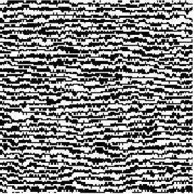
Figure 5: Typical spin configuration of the FFIM with the Zig-Zag coupling configuration when initially prepared at $T\rightarrow+\infty$ and then quenched at $T_{c}=0$.

In the case of homogeneous ferromagnets quenched below their critical temperature, domains grow with a characteristic length $L(t)$ behaving in time as $L(t)\sim t^{1/z}$ where $z=2$ is the dynamical exponent [17]. The two-time autocorrelation function of the local order parameter can be decomposed as

$$C(t,s)=C_{\rm st.}(t-s)+C_{\rm ag.}(t/s)$$ (4)

where $C_{\rm st.}(t-s)$ is due to reversible processes occurring inside the domains while $C_{\rm ag.}$ comes from the irreversible motion and annihilation of domain walls. This decomposition is clearly seen for example in the case of the spherical model [18]. Usually, the first term falls down rapidly and can be neglected. The self-similarity of the domain growth implies that two-time observables, say $C(t,s)$, depend only on $L(t)/L(s)$ and thus on $t/s$ when $1\ll s\sim t$, i.e. in the aging regime [4]. The autocorrelation function $C(t,s)$ behaves as [19, 20]:

$$C_{\rm ag.}(t,s)\sim M_{\rm eq}^{2}f_{C}\left({t\over s}\right)$$ (5)

with the scaling variable $t/s$. In the limit $t\gg s$, the scaling function $f_{C}(x)$ decays algebraically as $x^{-\lambda/z}$. This defines a new exponent, the autocorrelation exponent $\lambda$ [21]. At the critical point, similar conclusions can be drawn from the assumption that the correlation length grows during a quench as $\xi\sim t^{1/z_{c}}$. The autocorrelation function $C(t,s)$ displays a scaling behavior analogous to (5):

$$C_{\rm ag.}(t,s)\sim s^{-a_{c}}g_{C}\left({t\over s}\right)$$ (6)

where $g_{C}(x)$ is expected to decay asymptotically as $x^{-\lambda_{c}/z_{c}}$. Dynamical and autocorrelation exponents $z_{c}$ and $\lambda_{c}$ take values different from below $T_{c}$. Because $C(s,s)=\langle M^{2}(s)\rangle\sim\xi^{-2\beta/\nu}\sim s^{-2\beta/\nu z_{c}}$, the exponent $a_{c}$ is equal to ${2\beta/\nu z_{c}}$. The expression (6) works for a broad range of models for example the spherical model [18] or the Ising chain [22] that can be both treated analytically, the 2D Ising model by Monte Carlo simulations [18] or the $O(n)$ model analyzed by Renormalization Group technics [23]. In the case of the XY model, the motion of the domains is slowed down by the vortices that behave as impurities pinning the domain walls. The correlation length grows as $(t/\ln t)^{1/z_{c}}$ so that the autocorrelation function is modified by the replacement of the scaling variable $t/s$ by $t\ln s/s\ln t$ [24, 4]:

$$C_{\rm ag.}(t,s)\sim s^{-a_{c}}\tilde{g}_{C}\left({t\ln s\over s\ln t}\right)$$ (7)

We will analyze the aging of the FFIM in two steps. First, we will determine whether topological defects exist in the FFIM and affect the dynamics as claimed by some authors in the case of the AFIT. To that purpose, we will determine which one of the two scenarii (6) or (7) is the more compatible with our data, i.e. which scaling variable, $t/s$ or $t\ln s/s\ln t$, leads to a collapse of the scaling function $s^{a_{c}}C(t,s)$ for different waiting times $s$. Then, we will estimate the autocorrelation exponent $\lambda$ using the appropriate scaling variable. For these simulations, the lattice size is again $L=192$ with periodic boundary conditions but the data have been averaged over 50,000 different histories of the system.

3.1 Determination of the scaling variable

Our numerical estimation of the scaling function $s^{a_{c}}C(t,s)$ is plotted with respect to $t/s$ on Figure 6 and to $t\ln s/s\ln t$ on Figure 7. We used the exponent $a_{c}=0.2495(11)$ obtained in section 2. No collapse of the scaling function $s^{a_{c}}C(t,s)$ is observed with the scaling variable $t/s$ (Figure 6). The last two curves ($s=640$ and $1280$) are however closer to each other. Our waiting times $s$ are too small to check if this is the sign of an accumulation of the curves for much larger waiting times. In contradistinction, a very good collapse for large waiting times $s\geq 160$ can be seen in the inset of Figure 7 when the data are plotted versus $t\ln s/s\ln t$. The difference between the different curves is of the order of $2.10^{-3}$ where the correlation itself is of order of $0.2$. The difference between the different curves is of the order of magnitude of the statistical fluctuations of the data. For these reasons, it is unlikely that this collapse for the three waiting times $s=160$, $s=640$ and $1280$ be accidental and disappear for larger waiting times. We have also tried more complex scaling variables as $x=t(\ln s)^{\mu}/s(\ln t)^{\mu}$ or $x=t\ln{s\over t_{0}}/s\ln{t\over t_{0}}$ but they do not lead to a better collapse.

Note that the observation of these logarithmic corrections has been made possible by the use of the two times $t$ and $s$. It is well known that it is very difficult to distinguish these logarithmic corrections if ones studies only the asymptotic dependence of $C(t,s)$ on $t$, i.e. $C(t,s)\sim(t/\ln t)^{-\lambda/z}$. Moreover, if such corrections are observed, they may also result from corrections to scaling, i.e. $C(t,s)\sim t^{-\lambda/z}(1+at^{-\omega}+\ldots)$ with $\omega$ small. The relations (6) or (7) imposes a much stronger constraint than the asymptotic law $C(t,s)\sim(t/\ln t)^{-\lambda/z}$. We are looking for logarithmic factors in the scaling variable. The analysis is thus not sensitive to scaling corrections to the dominant algebraic decay. These considerations may explain why these logarithmic corrections, although observed by [7] for the AFIT have not be seen in more recent Monte Carlo simulations [5].

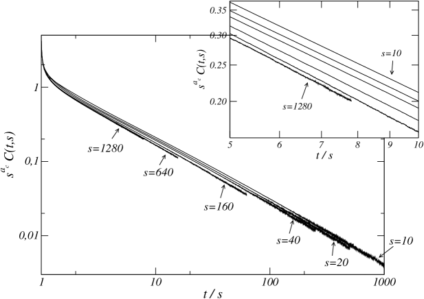
Figure 6: Scaling function $s^{a_{c}}C(t,s)$ of the spin-spin autocorrelation function versus $t/s$. The trend does not show any real trend to scaling.

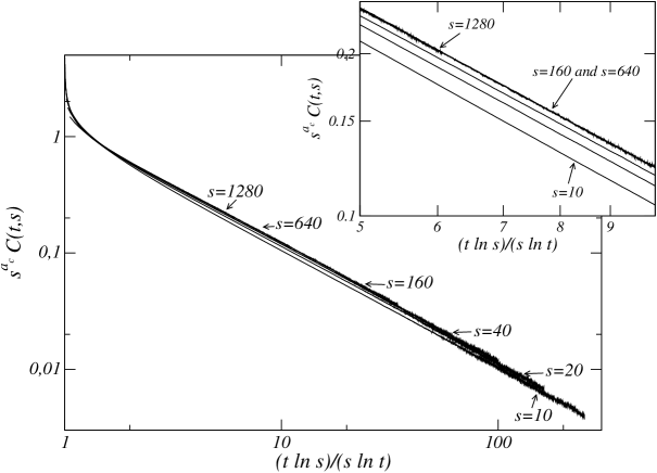
Figure 7: Scaling function $s^{a_{c}}C(t,s)$ of the spin-spin autocorrelation function versus $t\ln s/s\ln t$. A perfect collapse of the curve for the three largest waiting times can be observed in the inset.

3.2 Determination of the exponent $a_{c}$

The previous analysis relies strongly on the scaling form (5). Our conclusion may be criticized by arguing that corrections to the prefactor $s^{-a_{c}}$ should have been taken into account. To show that these corrections are negligible for the range of times $s$ and $t$ where we observe the collapse of the scaling function, we studied the two-time correlation $C(t,s)$ on the family of curves $t\ln s/t\ln s=\kappa$ where $\kappa$ is a constant. Along these curves, the scaling function $g_{C}(\kappa)$ is constant and the scaling form (5) reduces to $s^{-a_{C}}$. We then defined an effective exponent as

$$a_{\rm eff}(s_{1},s_{2})=-{\ln C(t_{2},s_{2})-\ln C(t_{1},s_{1})\over\ln s_{2}-\ln s_{1}}$$ (8)

where $t_{1}\ln s_{1}/t_{1}\ln s_{1}=t_{2}\ln s_{2}/t_{2}\ln s_{2}=\kappa$. In practice, to allow for non-integer values of $t_{1}$ and $t_{2}$ the logarithm of the autocorrelation function $C(t,s)$ was interpolated linearly between the two nearest simulation points, i.e. $\ln C(t,s)=(t-{\rm Int}\ \!t)\ln C({\rm Int}\ \!t,s)+(1-t+{\rm Int}\ \!t)\ln C({\rm Int}\ \!t+1,s)$ where ${\rm Int}\ \!t$ is the largest integer smaller or equal to $t$.

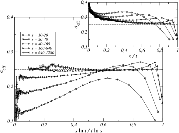
Figure 8: Effective exponent $a_{\rm eff}$ estimated by a fit of the correlation function as $C(t,s)\sim s^{-a_{c}}$. The time $t$ is chosen such that the scaling variable $t\ln s/s\ln t$ (or $t/s$ in the inset), and thus the scaling function $\tilde{g}_{C}$ in Eq. 7 ($g_{C}$ in Eq. 6), is kept constant. The legend indicates the two waiting times $(s_{1},s_{2})$ used for the calculation of the effective exponent.

The effective exponent is expected to tend to the exact value $a_{c}=0.25$ in the limit of large waiting times $s$. At finite values of $s$, corrections to the behavior $s^{-a_{c}}$ should lead to effective exponents that differ from $a_{c}=0.25$. Our data are plotted on Figure 8. One can see that the effective exponent displays as expected a plateau around the exact value $a_{c}=0.25$ when sufficiently large waiting times $s\geq 160$ are used. The same analysis have been performed along the curve $t/s=\kappa={\rm Cst}$. It leads to an effective exponent significantly larger than the exact value $a_{c}=0.25$. Moreover the absence of any plateau of the effective exponent excludes the possibility of a value of $a_{c}$ different from $0.25$. This analysis confirms that the scaling form that is the most compatible with our data is (7) and not (6).

3.3 Determination of the autocorrelation exponent $\lambda_{c}$

We are now interested in the autocorrelation exponent $\lambda_{c}$ defined by the assumption that the scaling function $\tilde{g}_{C}$ decays asymptotically as $\tilde{g}_{C}(x)\sim x^{-\lambda_{c}/z_{c}}$ where $x=t\ln s/s\ln t$ is the scaling variable. To take into account the possibility of corrections to this behavior, we studied the effective exponent $(\lambda_{c}/z_{c})_{\rm eff.}(x_{\rm min},x_{\rm max})$ defined as the decay exponent of the autocorrelation function $C(t,s)$ with $x=t\ln s/s\ln t$ in the window $x\in[x_{\rm min};x_{\rm max}]$. The upper bound $x_{\rm max}$ is the largest scaling variable allowed by our data, i.e. $x_{\rm max}=x(s,t=10000)$. The low bound of the interpolation range is varied between $x(s,s)=1$ and $x_{\rm max}$. The data are plotted with respect to $1/x_{\rm min}$ on Figure 9. For small values of $x_{\rm min}$, almost all numerical data, including small values of $x$, are included in the power-law interpolation. As a consequence, the corrections may play an important rôle and lead to an effective exponent possibly quite different from the asymptotic value $\lambda_{c}/z_{c}$. When $x_{\rm min}$ is increased, the effective exponent is expected to tend to $\lambda_{c}/z_{c}$. When $x_{\rm min}$ approaches $x_{\rm max}$, the number of points that contribute to the fit decreases and the effective exponent becomes noisier. The exponent $\lambda_{c}/z_{c}$ has to be estimated in an intermediate regime.

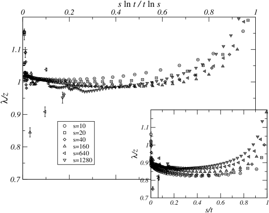
Figure 9: Effective exponent $\lambda_{c}/z_{c}$ obtained by a power-law fit $C(t,s)\sim x^{-\lambda_{c}/z_{c}}$ where $x$ is the scaling variable, i.e. $x=t\ln s/s\ln t$ (main figure) when taking into account topological defects and $x=t/s$ (insert) otherwise. The fit is performed in the range $x\in[x_{\rm min};x_{\rm max}]$ where $x_{\rm max}$ is the maximum value of the scaling variable allowed by our data. $x_{\rm min}$ is varied and the effective exponent $\lambda_{c}/z_{c}$ is plotted with respect to $1/x_{\rm min}$. Since we are interested in the asymptotic regime where corrections to scaling can be neglected, the interesting region corresponds to $x_{\rm min}$ large.

The data are plotted on Figure 9. For large values of $x_{\rm min}$, the effective exponent stays inside a range corresponding to $\lambda_{c}/z_{c}\simeq 1.02(2)$. This means that the autocorrelation exponent is $\lambda_{c}\simeq 2.04(5)$. and therefore appears to be saturated, i.e. $\lambda_{c}=d$. The ratio $\lambda_{c}/z_{c}$ remains compatible with our estimate $1.02(2)$ when considering more complex scaling variables involving logarithmic corrections as $x=t(\ln s)^{\mu}/s(\ln t)^{\mu}$ or $x=t\ln{s\over t_{0}}/s\ln{t\over t_{0}}$. The same procedure with the scaling variable $x=t/s$ leads to an incompatible estimate $(\lambda_{c}/z_{c})_{\rm eff}\simeq 0.91(2)$. This difference may be due to the fact that the asymptotic regime is seen only for larger times if one does not take into account logarithmic corrections. Note that the decay exponent $0.86$ was obtained for the AFIT when no logarithmic correction is considered [5]. One can thus assume that taking into account these corrections, an exponent closer to $1$ would have been obtained.

4 Conclusions

We have given numerical evidences in favor of the existence of topological defects in the paramagnetic phase of the FFIM. The dynamical exponent at the critical temperature $T_{c}=0$ is estimated to be $z=2.004(9)$, in excellent agreement with the value $z=2$ expected for the AFIT in the scenario involving topological defects [7] and fully incompatible with the Monte Carlo study where the signature of these topological defects was not seen. We have then studied the decay of the spin-spin autocorrelation function $C(t,s)$. Assuming that $C(t,s)$ scales as the homogeneous XY ferromagnet, a good collapse of the scaling function is observed for large waiting times. Moreover, the exponent $a_{c}$ is correctly obtained. This would not be the case if logarithmic corrections were not taken into account. Interestingly, the autocorrelation exponent is compatible with the simple value $\lambda_{c}=d$. Note that it is also the case for the Ising chain whose critical temperature is $T_{c}=0$ like the FFIM.

An important question remains unsolved: in the AFIT, the topological defects are known to be vortices. The couplings are not homogeneous in the FFIM so it is not obvious to us how these topological defects look like for this model. Unfortunately, they cannot be observed on snapshots of the spin configurations. Note that it is also the case for the AFIT. Moore et al. managed to pin vortices and make it observable by averaging over a large number of spin configurations. Without an idea of the shape of these topological defects in the FFIM, we have been unable to apply this procedure to the FFIM. Further investigation in this direction is necessary.

References

- [*] To whom all correspondence should be addressed. Electronic address: chatelai@lpm.u-nancy.fr
- [1] J.-P. Bouchaud, L.F. Cugliandolo, J. Kurchan, and M. Mezard, Out of equilibrium dynamics in spin-glasses and other glassy systems, in Spin-glasses and random fields, A.P. Young Ed. (World Scientific, 1997)
- [2] L.F. Cugliandolo, Dynamics in Glassy systems, Lecture Notes in Les Houches (2002) e-print cond-mat/0210312
- [3] A. Crisanti and F. Ritort, J. Phys A.: Math. Gen. 36, R181 (2003)
- [4] A.J. Bray, Adv. Phys. 43, 357 (1994)
- [5] E. Kim, B. Kim, and S.J. Lee, Phys. Rev. E 68 066127 (2003) ; E. Kim, S.J. Lee, and B. Kim, Phys. Rev. E 75 021106 (2007)
- [6] J. Kolafa, J. Phys. A 17 L777 (1984)
- [7] C. Moore, M.G. Nordahl, N. Minar, and C.R. Shalizi, Phys. Rev. E 60, 5344 (1999)
- [8] L. Berthier, P.C.W. Holdsworth, and M. Sellitto, J. Phys. A: Math. Gen. 34, 1805 (2000)
- [9] B. Nienhuis, H. J. Hilhorst, and H. W. J. Blöte, J. Phys. A 17, 3559 (1984)
- [10] D.C. Mattis, Phys. Lett. A 56, 421 (1976)
- [11] M.E. Fisher, Phys. Rev. 124, 1664 (1961)
- [12] J. Villain, J. Phys. C 10, 1717 (1977)
- [13] G. Forgacs, Phys. Rev. B 22, 4473 (1980)
- [14] G.H. Wannier, Phys. Rev. 79, 357 (1950)
- [15] R.J. Glauber, J. Math. Phys 4, 294 (1963)
- [16] D. Kandel, R. Ben-Av, and E. Domany, Phys. Rev. Lett. 65, 941 (1990) ; D. Kandel, R. Ben-Av, and E. Domany, Phys. Rev. B 45, 4700 (1992)
- [17] P.C. Hohenberg and B.I. Halperin, Rev. Mod. Phys. 49, 435 (1977)
- [18] C. Godrèche and J.-M. Luck, J. Phys. A 33, 9141 (2000)
- [19] H.K. Janssen, B. Schaub and B. Schmittmann, Z. Phys. B 73, 539 (1989)
- [20] C. Godrèche and J.-M. Luck, J. Phys. Cond. Matter 14, 1589 (2002)
- [21] D.S. Fisher and D. Huse, Phys. Rev. B 38, 373 (1988)
- [22] C. Godrèche and J.-M. Luck, J. Phys. A 33, 1151 (2000)
- [23] P. Calabrese and A. Gambassi, J. Phys. A 38, R133 (2005)
- [24] A.J. Bray and A.D. Rutenberg, Phys. Rev. E 49, R27 (1994)