Nonlinear coherent transport of waves in disordered media

Abstract

We present a diagrammatic theory for coherent backscattering from disordered dilute media in the nonlinear regime. The approach is non-perturbative in the strength of the nonlinearity. We show that the coherent backscattering enhancement factor is strongly affected by the nonlinearity, and corroborate these results by numerical simulations. Our theory can be applied to several physical scenarios like scattering of light in nonlinear Kerr media, or propagation of matter waves in disordered potentials.

It is already known that the interplay between disorder and - even very weak - nonlinearity can lead to dramatic changes to the system’s properties: for example, instabilities occur spivak ; skipetrov ; peter_tobias , or localization may be destroyed shepel . In the experiments studying the localization properties of matter waves in speckle potentials bec , the nonlinear regime, arising from the atomic interactions, is almost unavoidable. Furthermore, nonlinear behavior is easily observed in coherent backscattering experiments using cold atoms as scatterers thierry . As a third example, also the random laser exhibits nonlinearities which potentially influence the structure of localized laser modes cao . In all these cases, even if the systems are governed by simple nonlinear wave equations, a precise description of the impact of this nonlinearity on the interference effects altering the properties of diffuse wave propagation is still lacking. Since exact numerical calculations for realistic situations are at the border of or beyond actual computer capacities, one needs an efficient theory providing directly disorder averaged quantities. For this purpose, the present letter shows that the standard diagrammatic approach ishimaru ; vanderMark ; robert can be extended to the nonlinear regime. Using ladder and crossed-like diagrams, we will derive a nonlinear radiative transfer equation for the averaged wave intensity, and then calculate the interference corrections on top of the nonlinear solution.

The general frame where our approach can be applied is as follows: we assume a nonlinear wave equation with unique and stationary monochromatic solution. In particular, we assume that all even orders $\chi^{(n)}$, $n=2,4,\dots$, of the nonlinear susceptibility vanish, such that the generation of higher harmonics can be neglected. Furthermore, the refractive index modifications are small enough such that we can neglect effects like self-focusing, pattern formation and solitons boyd on the length scale set by the disorder (a mean free path). Instead, the nonlinear effects relevant for our disordered case can be summarized as follows: firstly, the wave intensity $I({\bf r})$ becomes a fluctuating quantity, which is especially important in the nonlinear regime. Secondly, the usual picture of weak localization resulting from interference only between pairs of amplitudes propagating along reversed paths breaks down in the nonlinear regime. As a consequence of the nonlinear mixing between different partial waves, weak localization must rather be interpreted as a multi-wave interference phenomenon wellens05 ; wellens06b . In particular, we will show in the following that the height of the coherent backscattering peak is strongly affected by nonlinearities, even if they do respect the reciprocity symmetry. In contrast to our previous work wellens05 ; wellens06b , the present approach is non-perturbative in the strength of the nonlinearity.

At first, we consider an assembly of $N$ point-like scatterers located at randomly chosen positions $\mathbf{r}_{i}$, $i=1,\dots,N$ inside a sample volume $V$ illuminated by a plane wave $\mathbf{k}_{L}$, with $|{\bf k}_{L}|=k$. We assume the field radiated by each scatterer to be a nonlinear function $f(E_{i})$ of the local field $E_{i}$. Since all even orders of the nonlinear susceptibilities vanish, we can write $f(E)=g(I)E$, where $I=EE^{*}$ is the local intensity, and $g(I)$ is proportional to the polarizability of the scatterers. This results in a set of nonlinear equations for the field at each scatterer:

$$E_{i}=e^{i\mathbf{k}_{L}\cdot\mathbf{r}_{i}}+\sum_{j\neq i}\frac{e^{ik|{\bf r}_{i}-{\bf r}_{j}|}}{4\pi|{\bf r}_{i}-{\bf r}_{j}|}g(E_{j}E_{j}^{*})E_{j}$$ (1)

As explained above, we aim at providing a theory providing the relevant quantities (local intensities, coherent backscattering cone…) averaged over the random positions of the scatterers. In a first step, we will derive an equation for the mean intensity $\langle I({\bf r})\rangle$. In the dilute regime, where the typical distances $|{\bf r}_{i}-{\bf r}_{j}|$ are much larger than the wavelength, we may neglect - in first approximation - correlations between the fields emitted by different scatterers. Under this condition, the scattered field $E_{d}({\bf r})$ is a superposition of spherical waves with random relative phases, depicting thus a speckle pattern. This leads to the well known Gaussian statistics for the complex field $E_{d}({\bf r})$ goodman , which is thus completely determined by a single parameter, the mean diffuse intensity $I_{d}({\bf r})=\langle|E_{d}({\bf r})|^{2}\rangle$. In addition to the scattered field, there is also a non-fluctuating coherent component originating directly from the incident field. In total, we have $E({\bf r})=E_{c}({\bf r})+E_{d}({\bf r})$, and the average intensity splits into a coherent and diffuse part: $\langle I({\bf r})\rangle=I_{c}({\bf r})+I_{d}({\bf r})$, with $I_{c}=|E_{c}|^{2}$. The mean density of radiation intensity emitted from point $\mathbf{r}$ is then given by:

$$K(\mathbf{r})=\mathcal{N}\left<ff^{*}\right>=\mathcal{N}\left<|g\left(I(\mathbf{r})\right)|^{2}I(\mathbf{r})\right>$$ (2)

where $\mathcal{N}=N/V$ denotes the density of scatterers, and the average $\left<\dots\right>$ is taken over the Gaussian statistics of the scattered field.

Between two scattering events, the wave propagates in an effective medium made by the scatterers. The corresponding refractive index $n$ and mean free path $\ell$ are not the same for the coherent and the diffuse fields, because of their different statistical properties combined with the nonlinear behavior of the scatterers. In the dilute regime, the diffuse amplitude can be considered as a weak probe, such that the complex refraction index reads:

$$n=1+\frac{\mathcal{N}}{2k^{2}}\left<\frac{df}{dE}\right>,\ \frac{1}{\ell}=2k{\rm Im}\{n\}$$ (3)

whereas, for the coherent mode, the derivative $d/dE$ is replaced by $1/E_{c}$, i.e. $n_{c}=1+\mathcal{N}\left<f\right>/(2k^{2}E_{c})$, and $1/\ell_{c}=2k{\rm Im}\{n_{c}\}$. Since the results of the averages depend on $I_{c}({\bf r})$ and $I_{d}({\bf r})$, the nonlinear refractive indices also attain a spatial dependence $n({\bf r})$ and $n_{c}({\bf r})$. They describe average propagation of one strong and many uncorrelated weak fields. (If there is more than one strong field, additional phenomena like four-wave mixing occur boyd .)

Recollecting all preceding ingredients, the transport equations for the average intensity read as follows:

$$I_{c}({\bf r}) = e^{-\overline{z/\ell_{c}}}$$ (4)

$$I_{d}({\bf r}) = \int_{V}d{\bf r^{\prime}}\frac{e^{-\overline{|{\bf r}-{\bf r^{\prime}}|/\ell}}}{(4\pi|{\bf r}-{\bf r^{\prime}}|)^{2}}K({\bf r^{\prime}})$$ (5)

Here, $z$ denotes the distance from the surface of $V$ to $\bf r$, in the direction of the incident beam. Furthermore, propagation from ${\bf r^{\prime}}$ to $\bf r$ implies a spatial average of $1/\ell({\bf r})$, which we note as follows: $\overline{|{\bf r}-{\bf r^{\prime}}|/\ell}:=|{\bf r}-{\bf r^{\prime}}|\int_{0}^{1}ds/\ell({\bf r}-s{\bf r}+s{\bf r^{\prime}})$, and similarly for the coherent mode ($\overline{z/\ell_{c}}$). Since $K$, $\ell$ and $\ell_{c}$ depend on $I_{c}({\bf r})$ and $I_{d}({\bf r})$, the above Eqs. (4,5) form two coupled integral equations, whose solution we find numerically. Finally, the intensity scattered into backwards direction (expressed as dimensionless quantity, the so-called ‘bistatic coefficient’ishimaru ) results as:

$$\Gamma_{L}=\int\frac{d{\bf r}}{4\pi A}e^{-\overline{z/\ell}}K({\bf r})$$ (6)

where $A$ denotes the transverse (with respect to the incident beam) area of the scattering volume $V$.

The validity of the preceding approach has been tested using the following nonlinear function:

$$g(I)=\frac{2\pi i}{k(1+\alpha I)}$$ (7)

which depicts the (elastic) nonlinear behavior of a two-level atom exposed to an intense laser beam. The nonlinear scatterers described by Eq. (7) are randomly distributed inside a sphere, with homogeneous density. We must emphasize that, for this particular model of nonlinearity, the stationary solution is always found to be unique and stable, as a consequence of the saturation $g(I)\to 0$ for large $\alpha$. From the numerical solution of Eq. (1), we calculate the radiated field and intensity outside the cloud in different directions $\theta$. This procedure is then repeated with many different configurations giving us the disorder averaged field and intensity. The results presented in this letter are obtained with 3000 configurations of $1500$ scatterers with density such that $k\ell=67$ and optical thickness $b=2$ (in the linear limit $\alpha=0$).

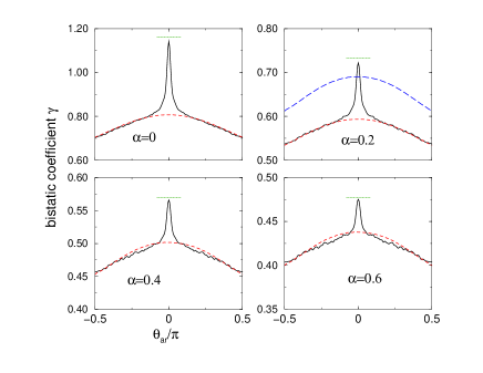
Figure 1: (Color online) Comparison between exact numerical calculations and the theoretical approach (see text for details). The solid line depict the exact numerical results, whereas the dashed line corresponds to $\Gamma_{L}$ including geometrical effects. The dotted line corresponds to the sum $\Gamma_{L}+\Gamma_{C}$ exactly in the backward direction. The additional curve (long dashed line) plotted for $\alpha=0.2$ depicts the results obtained when the fluctuating character of the diffuse field is not taken into account.

The results for the average intensity as a function of the backscattering angle $\theta$ are depicted in Fig. 1 for different values of the nonlinear parameter $\alpha=0$, $0.2$, $0.4$ and $0.6$. For each plot, the solid line depicts the exact numerical results, whereas the dashed line corresponds to $\Gamma_{L}$, Eq. (6), supplemented by a geometrical factor depending on $\theta$. Away from the backward direction, the agreement between the exact numerical calculations and our theoretical prediction for the background is clearly excellent. This is emphasized by the additional curve (long dashed line) plotted for $\alpha=0.2$ depicting the results obtained when neglecting the fluctuations of $I(\mathbf{r})$, for example replacing $\left<|g(I)|^{2}I\right>$ by $|g(\left<I\right>)|^{2}\left<I\right>$ in Eq. (2).

In the backward direction, constructive interference between reversed scattering paths results in the well-known coherent backscattering peak. As obvious from Fig. 1, the height of this peak is strongly affected by the nonlinearity. Nevertheless, we are perfectly able to incorporate these interferences effects in our approach, see the horizontal dotted lines in Fig. 1, which depict the predicted total bistatic coefficient, $\Gamma_{L}+\Gamma_{C}$, see Eq. (13) below, in the exact backward direction fullcone . These results are obtained by a diagrammatic analysis, which we summarize in the following.

As in the linear theory, we calculate the coherent backscattering effect by so-called ‘crossed’ or ‘cooperon’ diagrams vanderMark , describing pairs of reversed scattering paths. Hence, the individual scatterers are subject to two different incident probe fields $E$ and $E^{*}$, which represent the two amplitudes propagating along the reversed paths. The response of a scatterer to these two weak probe fields is given by the derivative $d^{2}/(dEdE^{*})$. Depending on whether the incident fields act on the dipole $f$ or its complex conjugate $f^{*}$, we obtain the four terms represented in Fig. 2(a-d).

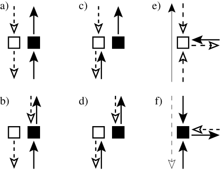
Figure 2: Building blocks for the diagrammatic calculation of nonlinear coherent backscattering. Filled squares (with outgoing solid arrows) denote the scattered field $f$, and open squares (with outgoing dashed arrows) the complex conjugate $f^{*}$. Incoming solid (dashed) arrows represent derivatives $d/dE$ ($d/dE^{*}$). Diagrams (a-d) contribute to the cooperon cross sections $\kappa$ and $\tilde{\kappa}$, see Eq. (8), whereas diagrams (e,f) represent nonlinear propagation $\tau^{*}$ and $\tau$, see Eq. (9).

If we denote the sum of diagram (a) + (c) by $\kappa$, and (b) + (d) by $\tilde{\kappa}$, the explicit expressions read:

$$\kappa=\mathcal{N}\left<\frac{d}{dE}\left(f\frac{df^{*}}{dE^{*}}\right)\right>,\ \tilde{\kappa}=\mathcal{N}\left<\frac{d}{dE}\left(f^{*}\frac{df}{dE^{*}}\right)\right>$$ (8)

If one of the incident fields originates from the coherent mode, $d/dE$ is again replaced by $1/E_{c}$, i.e. $\kappa_{c}=\mathcal{N}\left<fdf^{*}/dE^{*}\right>/E_{c}$ and $\tilde{\kappa}_{c}=\mathcal{N}\left<f^{*}df/dE^{*}\right>/E_{c}$.

Concerning propagation between two scattering events, the refractive index, Eq. (3), remains unchanged for the reversed paths. In addition to that, however, we find two other contributions shown in Fig. 2(e,f), which exist only as crossed diagrams. Here, diagram (e) represents the expression:

$$\tau=-\frac{i\mathcal{N}}{2k}\left<\frac{d^{3}f^{*}}{(dE^{*})^{2}dE}\right>$$ (9)

and diagram (f) its complex conjugate ($\tau^{*}$). For the coherent mode, the above expression is again modified as follows: $\tau_{c}=-i{\mathcal{N}}\left<d^{2}f^{*}/(dE^{*})^{2}\right>/(2kE_{c})$. The propagation of the thin line in Fig. 2(e,f) is unaffected by the nonlinear event.

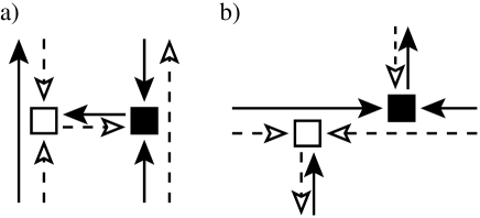
Figure 3: Examples of forbidden (a) and allowed (b) combinations of the building blocks shown in Fig. 2. The forbidden combinations correspond to those forming a closed loop in the sense that two squares are connected by two arrows pointing in different directions.

The crossed transport equation is established by connecting the building blocks shown in Fig. 2 with each other. As we have found, however, some combinations of diagrams represent unphysical processes which do not occur in the formal expansion of the solution of the nonlinear wave equation as a multiple scattering series. An example is shown in Fig. 3(a). The problem with this diagram is that the fields radiated by $f^{*}$ and $f$ mutually depend on one another. Therefore, one cannot tell which one of the two events $f$ or $f^{*}$ happens before the other one. This contradicts the multiple scattering series, where the individual scattering events occur one after the other. In order to avoid closed loops like the one shown in Fig. 3(a), we must ignore all combinations where one of the diagrams Fig. 2(c,d) or (e) occurs after Fig. 2(b,d) or (f) when following the solid arrow along the crossed path.

We account for these forbidden diagrams by splitting the transport equation into two parts, which we call $C_{1}$ and $C_{2}$. The first part, $C_{1}$, contains only diagrams Fig. 2(a,c) and (e). As soon as one of the events Fig. 2(b,d,f) occurs, the crossed intensity changes from type $C_{1}$ to type $C_{2}$. The subsequent propagation of $C_{2}$ is then given by diagrams Fig. 2(a,b,f). Following these rules, we describe the propagation of $C_{1,2}$ by transport equations similar to Eqs. (4,5):

$$C_{c}({\bf r}) = e^{ik\overline{z(n_{c}-n^{*})}}$$ (10)

$$C_{1}({\bf r}) = \int_{V}d{\bf r^{\prime}}P({\bf r},{\bf r^{\prime}})\Bigl{(}\sigma C_{1}+\sigma_{c}C_{c}\Bigr{)}({\bf r^{\prime}})$$ (11)

$$C_{2}({\bf r}) = \int_{V}d{\bf r^{\prime}}P({\bf r},{\bf r^{\prime}})\Bigl{(}\sigma^{*}C_{2}+\tilde{\sigma}C_{1}+\tilde{\sigma}_{c}C_{c}\Bigr{)}({\bf r^{\prime}})\ \ \$$ (12)

where the propagation kernel $P({\bf r},{\bf r^{\prime}})=\exp(-\overline{|{\bf r}-{\bf r^{\prime}}|/\ell})/(4\pi|{\bf r}-{\bf r^{\prime}}|)^{2}$ is the same as in Eq. (5), and the cross sections $\sigma$ result as follows: $\sigma=\kappa+\ell K\tau$, $\tilde{\sigma}=\tilde{\kappa}+\ell K\tau^{*}$ and, similarly, $\sigma_{c}=\kappa_{c}+\ell K\tau_{c}$ and $\tilde{\sigma}_{c}=\tilde{\kappa}_{c}+\ell K\tau_{c}^{*}$. Finally, the crossed bistatic coefficient reads:

$$\Gamma_{C}=\int_{V}\frac{d{\bf r}}{4\pi A}e^{ik\overline{z(n-n_{c}^{*})}}\Bigl{(}(\sigma_{c}^{*}+\tilde{\sigma}_{c}^{*})C_{1}+\sigma_{c}^{*}C_{2}\Bigr{)}({\bf r})$$ (13)

For comparison with the background $\Gamma_{L}$, we define diffuson cross sections by writing $K=\sigma^{(d)}I_{d}+\sigma^{(d)}_{c}I_{c}$, such that Eq. (5) attains a form comparable to Eq. (11). Exploiting the Gaussian properties of the diffuse field, we find: $\sigma^{(d)}={\mathcal{N}}\left<d(ff^{*})/dI\right>$ and $\sigma^{(d)}_{c}={\mathcal{N}}\left<d(ff^{*})/dE\right>/E_{c}^{*}$. Thus, the decrease of the backscattering peak observed in Fig. 1 is traced back to the fact that the cooperon cross sections $\sigma$ and $\tilde{\sigma}$ decrease faster than the diffuson cross section $\sigma^{(d)}$. Let us note that there also exist other models than Eq. (7), where our theory predicts an increasing coherent backscattering cone. However, these models might suffer from speckle instabilities - a point which requires further investigations.

To obtain the relatively simple form of Eqs. (10-13), we assume that the scattered intensity $K({\bf r})$ is approximately constant on length scales comparable to the mean free path $\ell$, and we neglect some diagrams where the coherent mode $C_{c}$ is affected by a nonlinear event $\tau_{c}$. These approximations are expected to be well fulfilled in the case of large optical thickness $b$. In the numerical comparison depicted in Fig. 1, where $b$ is not very large, we have used the exact version of Eqs. (10-13), which will be published elsewhere.

As explained in the introduction, our theoretical scheme also applies to other types of nonlinear systems, like, for example, the case of linear scatterers embedded in a homogeneous nonlinear medium:

$$\Delta E({\bf r})+k^{2}\Bigl{(}\epsilon({\bf r})+\alpha|E({\bf r})|^{2}\Bigr{)}E({\bf r})=0$$ (14)

with $\delta$-correlated disorder $\epsilon({\bf r})$ corresponding to a (linear) mean free path $\ell_{0}$. Here, the dilute medium approximation is valid if $k\ell_{0}\gg 1$ and $(\alpha I)^{2}k\ell_{0}\ll 1$. The latter condition is automatically fulfilled if we assume that we are in the stable regime, where Eq. (14) has a unique solution. According to skipetrov , this is the case (for $\alpha\in{\mathbbm{R}}$) if $(\alpha I)^{2}b^{2}(k\ell_{0}+b)<1$, with $b$ the optical thickness.

In this case, the diagrammatic method applies in the same way as described above. In particular, we obtain the following expressions for the cross sections:

$$\sigma({\bf r})=\sigma_{c}({\bf r})=\frac{4\pi}{\ell_{0}}\left[1+ik\ell_{0}\alpha\left(I_{c}({\bf r})+I_{d}({\bf r})\right)\right],$$ (15)

$\tilde{\sigma}=\tilde{\sigma}_{c}=-4\pi ik\alpha(I_{c}+I_{d})$, $\sigma^{(d)}=\sigma^{(d)}_{c}=4\pi/\ell_{0}$, and for the mean free paths $n=\langle\epsilon\rangle+\alpha(I_{c}+I_{d})+i/(2k\ell_{0})$ and $n_{c}=\langle\epsilon\rangle+\alpha(I_{c}/2+I_{d})+i/(2k\ell_{0})$. In the energy conserving case $\alpha\in{\mathbbm{R}}$, it can be shown that $C_{2}$ does not contribute to the real part of the backscattering coefficient $\Gamma_{C}$. Then, it follows from Eqs. (11) and (15), that the nonlinearity introduces a phase difference $\Delta\phi=Mk\ell_{0}\alpha I$ between reversed paths undergoing $M$ linear scattering events. Since $\langle M\rangle\propto b$, we predict a significant reduction of the coherent backscattering peak if $bk\ell_{0}\alpha I\simeq 1$ (which is still inside the stable regime if $k\ell_{0}$ is large).

In summary, we have extended the usual diagrammatic approach to take into account nonlinear effects for the coherent transport in disordered systems beyond the perturbative regime. The excellent agreement with direct numerical simulations emphasizes the validity of our approach. It readily applies for many different nonlinear wave equations. Eq. (14), for example, is mathematically equivalent to the Gross-Pitaeskii equation describing nonlinear propagation of matter waves in random potentials. In the latter case, this method will allow us to describe the localization properties of the mean field. Extending the present approach within the Bogolioubov framework, it will be possible to understand how these localization properties are affected by the non-condensed fraction of the atoms.

We thank D. Delande and C. Miniatura for fruitful discussions. T.W. acknowledges support from the DFG.

References

- (1) B. Spivak and A. Zyuzin, Phys. Rev. Lett. 84, 1970 (2000)
- (2) S.E. Skipetrov and R. Maynard, Phys. Rev. Lett. 85, 736 (2000)
- (3) T. Paul et al., Phys. Rev. A 72, 063621 (2005)
- (4) D. L. Shepelyansky, Phys. Rev. Lett 70, 1787 (1993)
- (5) D. Clément et al., Phys. Rev. Lett 95 170409 (2005); C. Fort et al., Phys. Rev. Lett. 95 170410 (2005); T. Schulte et al., Phys. Rev. Lett. 95 170411 (2005); L. Sanchez-Palencia et al., Phys. Rev. Lett. 98, 210401 (2007)
- (6) T. Chanelière et al., Phys. Rev. E 70 036602 (2004)
- (7) H. Cao, Waves Ranom Media 13 R1 (2003)
- (8) A. Ishimaru,Wave Propagation and Scattering in Random Media (Academic, New York, 1978), Vols. I and II
- (9) M. B. van der Mark, M. P. van Albada, and A. Lagendijk, Phys. Rev. B 37, 3575 (1988)
- (10) R. C. Kuhn et al., Phys. Rev. Lett. 95, 250403 (2005)
- (11) R. W. Boyd, Nonlinear Optics (Academic, San Diego, 1992).
- (12) T. Wellens, B. Grémaud, D. Delande, and C. Miniatura, Phys. Rev. E 71 055603(R) (2005); Phys. Rev. A 73 013802 (2006)
- (13) T. Wellens and B. Grémaud, J. Phys. B: At. Mol. Opt. Phys. 39, 4719 (2006)
- (14) J. W. Goodman, J. Opt. Soc. Am. 66, 1145 (1976)
- (15) Our theory predicts the full shape of the cone, but if the invariance by rotation is lost for the crossed intensities , leading to much larger linear systems.