Shear viscosity and Bose statistics:
Capillary flow above $\lambda$ point

Abstract

The gradual fall of the shear viscosity at $T_{\lambda}<T<2.8K$, observed in a liquid helium 4 flowing through a capillary, is examined. The disappearance of the shear viscosity in a capillary flow is a manifestation of superfluidity in dissipative phenomena, the onset mechanism of which is a subtle problem compared to that of superfluidity in non-dissipative phenomena. Applying the linear-response theory to the reciprocal of the shear viscosity coefficient $1/\eta$, we relate these two types of superfluidity using the Kramers-Kronig relation. As a result, we obtain a formula describing the influence of Bose statistics on the kinematic shear viscosity in terms of the susceptibility, without getting involved in the details of the dissipation mechanism of a liquid. Compared to an ordinary liquid, a liquid helium 4 above $T_{\lambda}$ has a $10^{-3}$ times smaller shear viscosity coefficient. Hence, although in the normal phase, it is already an anomalous liquid under the strong influence of Bose statistics. The coherent many-body wave function grows to an intermediate size between a macroscopic and a microscopic one, not as a thermal fluctuation but as a thermal equilibrium state. Beginning with bosons without the condensate, we make a perturbation calculation of its susceptibility with respect to the repulsive interaction. Using the above formula on the kinematic shear viscosity, we examine how, with decreasing temperature, the growth of the coherent wave function gradually suppresses the shear viscosity, and finally leads to a frictionless flow at the $\lambda$-point.

I Introduction

Superfluidity of a liquid helium 4 was first discovered in a flow through a narrow channel and a capillary kap . In an ordinary liquid, the shear viscosity causes the shear stress $F_{xy}$ between two adjacent layers moving at different velocities

$$F_{xy}=\eta\frac{\partial v_{x}}{\partial y},$$ (1)

where $\eta$ is the shear viscosity coefficient. In a narrow pipe with an inside radius $a$ and a length $L$, the field of velocity driven by the pressure difference $\Delta P$ has a form such as

$$v_{z}(r)=\frac{a^{2}-r^{2}}{4\eta}\frac{\Delta P}{L},$$ (2)

where $r$ is a radius in the cylindrical coordinates (Poiseuille flow). In the superfluid phase of a liquid helium 4, even when the pressure difference vanishes ($\Delta P=0$), one observes a non-vanishing flow ($v_{z}(r)\neq 0$), hence $\eta=0$ in Eq.(2).

The shear viscosity of a liquid helium 4 has been subjected to considerable experimental and theoretical studies. At $0<T<T_{\lambda}$, an oscillating or rotating probe immersed in a liquid helium 4 experiences the shear stress in a complicated manner (viscosity paradox). At temperatures well below $T_{\lambda}$, various excitations of a liquid are strictly suppressed except for phonons and rotons. Hence, it is natural to assume that phonons and rotons are responsible for the shear viscosity. By regarding these elementary excitations as a weakly interacting dilute Bose gas, the formula in the kinetic theory of gases well describes the shear viscosity of a liquid at $T\ll T_{\lambda}$, which is a success of the quasi-particle picture in the many-body theory kha .

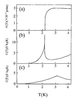
Figure 1: (a) The temperature dependence of the shear viscosity $\eta(T)$ of a liquid helium 4 measured in a flow through a capillary (after the data in Ref.3 and 5). (b) The temperature dependence of the specific heat $C(T)$ of a liquid helium 4 (after Atkins, Liquid helium4, (Cambridge,1959)). (c) $C(T)$ of an ideal Bose gas with the same density as a liquid helium 4.

For the shear viscosity at $T>T_{\lambda}$, however, the dilute-gas picture must not be applied, because the macroscopic condensate has not yet developed. Instead, one must tackle the problem of how Bose statistics affects excitations and dissipations of a liquid. Figure 1(a) shows $\eta$ of a liquid helium 4 measured in a flow through a capillary at the vicinity of $T_{\lambda}$ men tje zin . One notes that $\eta$ does not abruptly drops to zero at $T_{\lambda}$, but it gradually decreases with decreasing temperature from $T_{\lambda}+0.7K$, in which the macroscopic condensate has not yet developed, and finally drops at the $\lambda$-point.

For the shear viscosity of a liquid, Maxwell obtained a simple formula $\eta=G\tau$ (Maxwell’s relation), where $G$ is the modulus of rigidity and $\tau$ is a relaxation time, using a physical argument max (see Appendix.A). In the short time scale, a liquid shows similar behaviors to that of a solid at the molecular level. In a liquid, $G$ is determined mainly by the motion of vacancy as well as in a solid. Since no apparent structural transformation is observed in a liquid helium 4 at the vicinity of $T_{\lambda}$, $G$ may be a constant at the first approximation. The gradual decrease of $\eta=G\tau$ above $T_{\lambda}$ suggests that the influence of Bose statistics gives rise to a considerable decrease of $\tau$. To understand superfluidity occurring in such a dissipative flow, we must deal with the microscopic mechanism of the dissipations determining $\tau$. At first sight, it seems to be a hopeless attempt, because the dissipation itself is a complicated phenomenon allowing no simple description han . In a superfluid helium 4, many features associated to Bose statistics are masked by the strongly interacting character of the liquid. But, from a different viewpoint, new physics must lie in the phenomena in which Bose statistics is deeply entwined with the structure and dynamics of a liquid. Hence, we must find a starting point for disentangling these complicated problems. For the shear viscosity, we find such a starting point, in which one can consider one problem separately from the other ones.

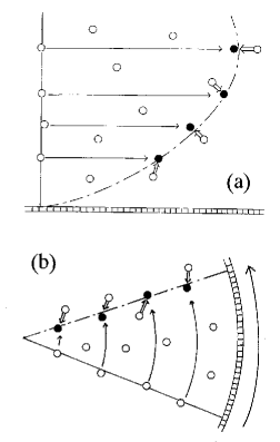
Figure 2: Two types of flows. (a) a flow through a capillary. (b) a rotational flow in a container. White circles represent an initial distribution of particles. The long arrows move white circles on a solid line to black circles. In both (a) and (b), permutation symmetry holds over the whole liquid at $T<T_{\lambda}$. The particles represented by black circles are reproduced by slight displacements by short arrows from the initial particles close to that particle.

The viscosity has a formally similar expression to other processes of diffusion, such as diffusion of matters and thermal conduction. The latter are the diffusion of a scalar quantity such as density $\rho$ and temperature $T$, and are always dissipative processes, whereas the viscosity is the diffusion of a vector quantity, momentum $p$. Since the vector field $m\mbox{\boldmath$v$}(\mbox{\boldmath$r$})$ has various spatial patterns, the viscosity has a qualitatively different feature that is not seen in diffusion of matters and thermal conduction. Figure 2 schematically illustrates two types of flows:(a) a flow in a capillary, and (b) a rotational flow in a container. In fluid dynamics, the viscous dissipation in an incompressible fluid is estimated by the dissipation function

$$\Phi(\mbox{\boldmath$r$})=2\eta\left(e_{ij}-\frac{1}{3}e_{kk}\delta_{ij}\right)^{2},$$ (3)

($e_{ij}=(\partial v_{i}/\partial x_{j}+\partial v_{j}/\partial x_{i})/2$ is the shear velocity). Particles in a capillary flow like Fig.2(a) experiences thermal dissipation not only at the boundary, but also in a flow. (For Poiseuille flow Eq.(2), the dissipation function Eq.(3) is not zero at any $r$ except for $r=0$.) On the other hand, in a rotating cylindrical container like Fig.2(b), a liquid makes the rigid-body rotation owing to its viscosity, the velocity of which is proportional to the radius and the rotational velocity $\Omega$ such as $\mbox{\boldmath$v$}_{d}(\mbox{\boldmath$r$})\equiv\mbox{\boldmath$\Omega$}\times\mbox{\boldmath$r$}$ . Except at the boundary to the wall, there is no frictional force within a liquid, and the flow is therefore a non-dissipative one. (For $v_{\phi}(r)=\Omega r$, Eq.(3) is zero at any $r$.) When we discuss the onset mechanism of superfluidity in such a non-dissipative flow, we can take an advantage of this feature to avoid dealing with the dissipation mechanism.

In this paper, we will consider the frictionless capillary flow of a liquid helium 4 by relating it with the nonclassical rotational flow using the Kramers-Kronig relation. (The former is superfluidity as a non-equilibrium process, whereas the latter is superfluidity as a thermal equilibrium one.) This method originated in studies of electron superconductivity. Just after the advent of BCS model, an attempt was made to relate the electrical conductivity (more precisely, the micro-wave absorption spectrum) with the penetration depth in the Meissner effect fer ttin . The former is a quantity in the dissipative phenomenon, and the latter is that in the non-dissipative one. Furthermore, the Meissner effect has a common mechanism with the nonclassical rotational flow of a Bose liquid noz . Hence, in the relationship between the electrical conduction and the Meissner effect in superconductivity, one finds a parallelism to that between the capillary flow and the rotational flow in a liquid helium 4. By using this analogy, one can consider the influence of Bose statistics on the shear viscosity of a liquid without getting involved in details of the dissipation mechanism of a liquid. Furthermore, one can explore the relationship between two typical manifestations of superfluidity .

Before carrying out this program, one must have a physical image on the gradual fall of $\eta$ at $T_{\lambda}<T<2.8K$ observed in a liquid helium 4 (Fig.1(a)). It has been assumed to be a manifestation of the thermal fluctuation of Boson systems, and discussed in connection with the $\lambda$-shape of the specific heat $C(T)$ (Fig.1(b)). The principal peak in $C(T)$ reflects thermal fluctuation in the critical region ahl . A peculiar feature of the $\lambda$-shape of $C(T)$ is that in addition to the sharp peak, the specific heat displays a symptom of its rise to the sharp peak already at $T_{\lambda}<T<T_{\lambda}+0.7K$, which suggests the cause of the gradual fall of the shear viscosity in the same temperature region. A remarkable fact is that an ideal Bose gas with the same density as the liquid helium 4 shows a similar gradual rise of $C(T)$ around $T_{c}$ as in Fig.1(c). Normally, the enhanced thermal fluctuation at the vicinity of $T_{c}$ comes from strong competitions between the interaction energy and the entropy effect, and occurs only within the very narrow temperature region around $T_{c}$. Hence, it is questionable to apply the concept of thermal fluctuation to this gradual rise of the specific heat at $T_{\lambda}<T<2.8K$, because of the following reasons: (1) it occurs in a far wider temperature region than the critical one, and (2) $C(T)$ of an ideal Bose gas suggests that it really occurs even if there is no particle interactions. Since the gradual fall of $\eta(T)$ above $T_{\lambda}$ may come from the same mechanism as the gradual rise of $C(T)$ above $T_{\lambda}$, the thermal fluctuation is a questionable interpretation for both phenomena. (This interpretation of the $\lambda$-shape of $C(T)$ leads us to reconsider the nature of the $\lambda$ transition and the meaning of the infinite volume limit. See Sec.5A.)

Compared to an ordinary liquid, a liquid helium 4 above $T_{\lambda}$ has a $10^{-3}$ times smaller shear viscosity coefficient. Although in the normal phase, it is already an anomalous liquid under the strong influence of Bose statistics. Hence, it seems natural to assume that large but not yet macroscopic coherent wave functions gradually grows as a thermal equilibrium state as $T\rightarrow T_{\lambda}$ in the normal phase, and suppresses the shear viscosity lod mat . (At an early stage in the study of superfluidity, R.Bowers and K.Mendelssohn discussed a similar view on the nature of the decrease of $\eta$ above $T_{\lambda}$ men .) The existence of such wave functions must affect the non-dissipative flow as well, such as the rotational flow above $T_{\lambda}$. Recently, from this viewpoint, the rotational property of a liquid helium 4 above $T_{\lambda}$ is theoretically examined koh , and a slight decrease of the moment of inertia above $T_{\lambda}$ is predicted. (The similar phenomenon occurs in the Meissner effect of the charged Bose gas as well kohmei .)

Experimentally, although a lot of measurements have been done on superfluidity of a liquid helium 4, there is so little direct experimental information about flow patterns. Among various visualization techniques used in ordinary liquids, particle image velocimetry (PIV), which records the motion of micrometre-scale solid particles suspended in the fluid as tracer particles, recently becomes available in a superfluid helium 4 don van . Using this technique, we will be able to closely compare the theory and the experiment on the onset mechanism of superfluidity.

In this paper, after formulating the shear viscosity of a liquid, we generalize the result of Ref.14 to the capillary flow. Since we focus on the continuous change of the system around $T_{\lambda}$, we cannot assume from the beginning the sudden emergence of the macroscopic condensate at $T_{\lambda}$. Rather, beginning with the system without the condensate, we consider the Bose system above and below $T_{\lambda}$ on a common ground, and study the intricacy underlying the onset of superfluidity.

This paper is organized as follows. Section 2.A considers the shear viscosity of a liquid by relating the dissipative flow to the non-dissipative ones using Kramers-kronig relation, and obtains a formula describing the influence of Bose statistics on the dissipative flow. Section.2.B discusses the physical reason that Bose statistics suppresses the shear viscosity. Beginning with the Bose system without the condensate, Sec.3 formulates a perturbation expansion of the susceptibility with respect to the repulsive interaction. By taking peculiar diagrams obeying Bose statistics in the above formula, Sec.3 examines how the growth of the coherent wave function gradually suppresses the shear viscosity at $T>T_{\lambda}$. Section 4 makes a comparison to experiments, and Sec.5 discusses the nature of the $\lambda$ transition, compare the dissipative and the non-dissipative flows, and makes a brief comment on the shear viscosity of Fermi liquids.

II Shear viscosity of a Bose liquid

II.1 Formalism of the shear viscosity of a liquid

For a liquid helium 4, the repulsive particle picture is not so unrealistic as it would be for any other liquid. Hence, as its simplest model, we use

$$H=\sum_{p}\epsilon(p)\Phi_{p}^{\dagger}\Phi_{p}+U\sum_{p,p^{\prime}}\sum_{q}\Phi_{p-q}^{\dagger}\Phi_{p^{\prime}+q}^{\dagger}\Phi_{p^{\prime}}\Phi_{p},\qquad(U>0),$$ (4)

where $\Phi_{p}$ denotes an annihilation operator of a spinless boson.

In the linear response theory, the shear viscosity coefficient is given by the following two-time correlation function of the stress tensor $J_{xy}(t)$

$$\eta=\frac{1}{Vk_{B}T}\int_{0}^{\infty}dt<J_{xy}(t)J_{xy}(0)>.$$ (5)

In a liquid, the particle interaction $U$ enhances not only a few-particle or collective excitations but also their relaxations, hence reducing the relaxation time $\tau$, and the shear viscosity coefficient $\eta=G\tau$. In principle, the shear viscosity coefficient of a liquid must be obtained by calculating an infinite series of the perturbation expansion of Eq.(5) kad . The interaction $U$ affects the imaginary part of the self energy of particles, thus changing the stress tensor $J_{xy}$. To obtain the resulting change of $<J_{xy}(t)J_{xy}(0)>$, one must know the dissipation mechanism of a liquid. In contrast with the case of a gas, the mechanism responsible for the shear viscosity in a liquid is similar to the vacancy motion in a solid, and is therefore a highly inhomogeneous process in the microscopic scale. Hence, it is difficult to derive the shear viscosity of a liquid without using any phenomenological model jeo .

Instead of $\eta$, however, if we apply the linear-response theory to its reciprocal $1/\eta$, and make the perturbation expansion with respect to $U$, the increase of $U$ naturally leads to the decrease of $\eta$ , thus naturally describing the effect of $U$ on $\eta$. Along this line of thought, we regard Eq.(2) of the Poiseuille flow, in which $\eta$ appears in the denominator, as a macroscopic linear-response formula. Without loss of generality, we may focus on a flow velocity at a single point. Using the flow velocity on the axis of rotational symmetry (z-axis), we define a current $\mbox{\boldmath$j$}=\rho\mbox{\boldmath$v$}(r=0)$ on the z-axis, and obtains

$$\mbox{\boldmath$j$}=-\sigma a^{2}\frac{\Delta\mbox{\boldmath$P$}}{L},\qquad\sigma=\frac{\rho}{4\eta},$$ (6)

where $\sigma$ is the conductivity of a liquid in a capillary flow ($\mbox{\boldmath$P$}=P\mbox{\boldmath$e$}_{z}$). Equation.(6) is a longitudinal linear response of a liquid to $\Delta\mbox{\boldmath$P$}/L$, which includes the dissipation by the shear viscosity cur . The perturbation expansion of $\sigma$ with respect to $U$ properly incorporates to $\eta$ the strong-coupling nature of a liquid.

Let us generalize Eq.(6) to the case of the oscillatory pressure gradient as follows

$$\mbox{\boldmath$j$}(\omega)=-\sigma(\omega)a^{2}\frac{\Delta\mbox{\boldmath$P$}(\omega)}{L}.$$ (7)

The Navier-Stokes equation gives an expression of the conductivity spectrum $\sigma(\omega)$ (see Appendix.B). By definition, $\sigma(\omega)$ in Eq.(7) must contain the mass $m$ of particles. Specifically, $\sigma(\omega)$ satisfies the following sum rule sum

$$\frac{1}{\pi}\int_{0}^{\infty}\sigma(\omega)d\omega=nm,$$ (8)

where $n$ is the number density of particles.

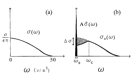
Figure 3: The change of the conductivity spectrum $\sigma(\omega)$ from (a) at $T>T_{\lambda}$ to (b) at $T<T_{\lambda}$. At $T>T_{\lambda}$, $\sigma(\omega)$ is given by Eq.(B5). At $T<T_{\lambda}$, $\omega_{s}$ is a half width of the sharp peak around $\omega=0$ with an area $A$, and $\omega_{c}$ is a frequency at the broad peak in $\sigma_{n}(\omega)$.

At $T<T_{\lambda}$, a frictionless flow appears in Eq.(7). Characteristic to the frictionless flow is the fact that in addition to the normal fluid part $\sigma_{n}(\omega)$, the conductivity spectrum $\sigma(\omega)$ has a sharp peak around $\omega=0$ (with a very small but finite half width $\omega_{s}$), while satisfying Eq.(8). Hence, one obtains

$$\mbox{\boldmath$j$}(\omega)=-\left[\sigma_{n}(\omega)+A\delta(\omega)\right]a^{2}\frac{\Delta\mbox{\boldmath$P$}(\omega)}{L},$$ (9)

where $\delta(\omega)$ is a simplified expression of the sharp peak around $\omega=0$, and $A$ is an area of this peak fer . Figure 3 schematically illustrates such a change of $\sigma(\omega)$ when the system passes $T_{\lambda}$. When $\sigma(\omega)$ has a form of $\sigma_{n}(\omega)+A\delta(\omega)$, one obtains the shear viscosity coefficient $\eta$ in Eq.(6) as

$$\eta(T)=\frac{1}{4}\frac{\rho}{\sigma_{n}(0)+\displaystyle{\left(\frac{A}{\omega_{s}}\right)}}.$$ (10)

In view of Eq.(10), the sharpness of the peak around $\omega=0$ ($\omega_{s}\simeq 0$) leads to the disappearance of the shear viscosity ($\eta(T)\simeq 0$) at $T<T_{\lambda}$.

Let us generalize Eq.(7) so that it includes not only the current responding in phase with $\Delta\mbox{\boldmath$P$}(\omega)$ but also a current responding out of phase. $\sigma(\omega)$ in Eq.(7) is generalized to a complex number $\sigma_{1}+i\sigma_{2}$ as follows

$$\mbox{\boldmath$j$}(\omega)=-\left[\sigma_{1}(\omega)+i\sigma_{2}(\omega)\right]a^{2}\frac{\Delta\mbox{\boldmath$P$}(\omega)}{L},$$ (11)

where $\sigma(\omega)$ in Eq.(7) is replaced by $\sigma_{1}(\omega)$. Causality states in Eq.(11) that only after the pressure gradient is applied, one observes a current, and obtains the following Kramers-Kronig relation

$$\sigma_{1}(\omega^{\prime})=\frac{2}{\pi}\int_{0}^{\infty}d\omega\frac{\omega\sigma_{2}(\omega)}{\omega^{2}-\omega^{\prime 2}},$$ (12)

$$\sigma_{2}(\omega^{\prime})=-\frac{2\omega^{\prime}}{\pi}\int_{0}^{\infty}d\omega\frac{\sigma_{1}(\omega)}{\omega^{2}-\omega^{\prime 2}}.$$ (13)

We will embed Eq.(11) in a more general picture, and derive properties of a capillary flow by regarding it as a special case. Instead of $\Delta\mbox{\boldmath$P$}(\omega)$, we use a quantity directly specifying the state of the system, that is, the velocity field $\mbox{\boldmath$v$}(t)$. Applying the pressure gradient to a liquid is equivalent to assuming the velocity field $\mbox{\boldmath$v$}(t)$ satisfying the equation of motion

$$\frac{d\mbox{\boldmath$v$}(t)}{dt}=-\frac{\Delta\mbox{\boldmath$P$}(t)}{L},$$ (14)

as an external field vec .

Let us consider a rotational flow like Fig.2(b). We assume $\mbox{\boldmath$v$}_{d}(\mbox{\boldmath$r$},t)=\mbox{\boldmath$\Omega$}\times\mbox{\boldmath$r$}e^{i\omega t}$ of the rigid-body rotation. In the rotational flow, $\mbox{\boldmath$j$}(\mbox{\boldmath$r$},\omega)$ and $\mbox{\boldmath$v$}_{d}(\mbox{\boldmath$r$},\omega)$ form the perturbation energy like $\int dx\mbox{\boldmath$v$}_{d}\cdot\mbox{\boldmath$j$}$. Since the rotational flow is a non-dissipative system, $\mbox{\boldmath$j$}(\mbox{\boldmath$r$},\omega)$ is a dynamical response of a liquid to the mechanical external field $\mbox{\boldmath$v$}_{d}(\mbox{\boldmath$r$},\omega)$, such as $\mbox{\boldmath$j$}(\mbox{\boldmath$r$},\omega)=\chi(\mbox{\boldmath$r$},\omega)\mbox{\boldmath$v$}_{d}(\mbox{\boldmath$r$},\omega)$, where $\chi(\mbox{\boldmath$r$},\omega)$ is the susceptibility of the system noz . Replacing $\Delta\mbox{\boldmath$P$}(\omega)/L$ with $-i\omega\mbox{\boldmath$v$}(\omega)$ in Eq.(11), we interchange the real and imaginary part of the coefficient in Eq.(11), and make it a local equation as follows

$$\mbox{\boldmath$j$}(q,\omega)=\left[-\omega\sigma_{2}(q,\omega)+i\omega\sigma_{1}(q,\omega)\right]a^{2}\mbox{\boldmath$v$}(q,\omega).$$ (15)

Equation (15) is a general formula including not only $i\omega\sigma_{1}(q,\omega)$ for the dissipative flow (Fig.2(a)), but also $-\omega\sigma_{2}(q,\omega)$ for the non-dissipative one (Fig.2(b)). If one determines $\sigma_{2}(q,\omega)$ in the non-dissipative flow, one obtains $\sigma_{1}(q,\omega)$ using Eq.(12) at a given $q$.

In the rotational flow, because of $div\mbox{\boldmath$v$}_{d}(\mbox{\boldmath$r$},t)=0$, $\mbox{\boldmath$v$}_{d}(\mbox{\boldmath$r$},t)$ acts as a transverse-vector probe to the excitation of bosons. This fact allows us a formal analogy with the vector potential $\mbox{\boldmath$A$}(\mbox{\boldmath$r$})$ in the Coulomb gauge ($div\mbox{\boldmath$A$}(\mbox{\boldmath$r$})=0$) acting on the charged Bose system. Hence, the neutral Bose system has a similar form of current to that of the charged Bose system noz such as

$$J_{\mu}(q,\tau)=\sum_{p,n}\left(p+\frac{q}{2}\right)_{\mu}\Phi_{p}^{\dagger}\Phi_{p+q}e^{-i\omega_{n}\tau},$$ (16)

($\hbar=1$ and $\tau=it$). Within the linear response, one obtains the generalized susceptibility

$$\chi_{\mu\nu}(q,\omega_{n})=\frac{1}{V}\int_{0}^{\beta}d\tau\exp(i\omega_{n}\tau)<G|T_{\tau}J_{\mu}(q,\tau)J_{\nu}(q,0)|G>,$$ (17)

where $|G>$ is the ground sate flu . Generally, the susceptibility is decomposed into the longitudinal and transverse part ($\mu=x,y,z$)

$$\chi_{\mu\nu}(q,\omega)=\frac{q_{\mu}q_{\nu}}{q^{2}}\chi^{L}(q,\omega)+\left(\delta_{\mu\nu}-\frac{q_{\mu}q_{\nu}}{q^{2}}\right)\chi^{T}(q,\omega).$$ (18)

For the later use, we define a term proportional to $q_{\mu}q_{\nu}$ in $\chi_{\mu\nu}$ by $\hat{\chi}_{\mu\nu}$

$$\chi_{\mu\nu}(q,\omega) = \delta_{\mu\nu}\chi^{T}(q,\omega)+q_{\mu}q_{\nu}\left(\frac{\chi^{L}(q,\omega)-\chi^{T}(q,\omega)}{q^{2}}\right)$$ (19)

$$\equiv \delta_{\mu\nu}\chi^{T}(q,\omega)+\hat{\chi}_{\mu\nu}(q,\omega),$$

where $\hat{\chi}_{\mu\nu}$ represents the balance between the longitudinal and transverse susceptibility wha . In the rotational flow, the influence of the wall motion propagates along the radial direction, which is perpendicular to the particle motion driven by rotation as illustrated in Fig.2(b). Hence, the rotational motion is a transverse response described by the transverse susceptibility $\chi^{T}(q,\omega)$. In the right-hand side of Eq.(15), the real part $-a^{2}\omega\sigma_{2}(q,\omega)$ of the coefficient describes the rotational motion as a non-dissipative response such as

$$-a^{2}\omega\sigma_{2}(q,\omega)=\chi^{T}(q,\omega),$$ (20)

and the imaginary part $a^{2}\omega\sigma_{1}(q,\omega)$ describes the dissipation.

Let us focus on the capillary flow. Using Eq.(20) in the right-hand side of Eq.(12) at a given $q$, one obtains

$$a^{2}\sigma_{1}(q,\omega^{\prime})=-\frac{2}{\pi}\int_{0}^{\infty}d\omega\frac{\chi^{T}(q,\omega)}{\omega^{2}-\omega^{\prime 2}}.$$ (21)

The slow excitations ($\omega\simeq 0$) in $\chi^{T}(q,\omega)$ of Eq.(21) are important for determining $\sigma_{1}(q,\omega)$. On this point, Eq.(21) has different interpretations in the normal and the superfluid phase. In the normal fluid phase, $\chi^{L}(q,\omega)=\chi^{T}(q,\omega)$ is satisfied at small $q$ and $\omega$, and one can replace $\chi^{T}(q,\omega)$ in Eq.(21) by $\chi^{L}(q,\omega)$ at a small $q$ and $\omega$ def . Hence, the conductivity $\sigma_{1n}(q,\omega)$ of a capillary flow in the normal fluid phase is given by

$$a^{2}\sigma_{1n}(q,\omega^{\prime})=-\frac{2}{\pi}\int_{0}^{\infty}d\omega\frac{\chi^{L}(q,\omega)}{\omega^{2}-\omega^{\prime 2}}.$$ (22)

In the superfluid phase, under the strong influence of Bose statistics, the condition of $\chi^{L}(q,\omega)=\chi^{T}(q,\omega)$ at $q\rightarrow 0$ is violated in the low-energy region extending from $\omega$ =0 (see Sec.2.B). (Furthermore, the rigidity of superfluidity requires that the nonzero $\chi^{L}(q,\omega)-\chi^{T}(q,\omega)$ depends on $q$ and $\omega$ very weakly at small $q$ and $\omega$.) Consequently, one cannot replace $\chi^{T}(q,\omega)$ by $\chi^{L}(q,\omega)$ in Eq.(21). For $\sigma_{1}(q,\omega)$, in addition to $\sigma_{1n}(q,\omega)$, one must separately consider the contribution of $\chi^{T}(q,\omega)-\chi^{L}(q,\omega)$. For $\sigma_{1}(0,\omega)$ of the capillary flow, one obtains

$$\sigma_{1}(\omega^{\prime})=\sigma_{1n}(\omega^{\prime})+\frac{2}{\pi a^{2}}\int_{0}^{\infty}d\omega\frac{\lim_{q\to 0}[\chi^{L}(q,\omega)-\chi^{T}(q,\omega)]}{\omega^{2}-\omega^{\prime 2}},$$ (23)

where we replace $\chi^{L}(q,\omega)-\chi^{T}(q,\omega)$ by its limit at $q\rightarrow 0$. Since this limit depends on $\omega$ very weakly at small $\omega$, we take out it from the integral with the aid of

$$\int_{0}^{\infty}\frac{d\omega}{\omega^{2}-\omega^{\prime 2}}=\delta(\omega^{\prime}),$$ (24)

and obtains

$$\sigma_{1}(\omega)=\sigma_{1n}(\omega)+\frac{2}{\pi a^{2}}\lim_{q\to 0}[\chi^{L}(q,0)-\chi^{T}(q,0)]\delta(\omega).$$ (25)

Comparing Eq.(25) with Eq.(9), one obtains an expected form of $\sigma(\omega)$ for the superfluid flow with $A=2\lim_{q\to 0}[\chi^{L}(q,0)-\chi^{T}(q,0)]/(\pi a^{2})$. If superfluidity was perfectly rigid to any perturbations, $\lim_{q\to 0}[\chi^{L}(q,\omega)-\chi^{T}(q,\omega)]$ would have no frequency dependence. In reality, this limit weakly depends on $\omega$ in Eq.(23). Hence, although the peak is well approximated by $\delta(\omega)$ in Eq.(25), it has a small but finite half width $\omega_{s}$ as in Fig.3(b), which represents a degree of the rigidity of superfluidity.

The change of $\sigma(\omega)$ from Fig.3(a) to 3(b) occurs under the sum rule Eq.(8). The area $A$ of the sharp peak is equal to that of the shaded region in Fig.3(b). We approximate this shaded region by a triangle. (A broad peak of $\sigma_{n}(\omega)$ is located at $\omega_{c}$). At $\omega=0$, the conductivity is enhanced by the sharp peak as $A/\omega_{s}$, but the original $\sigma(0)$ changes to $\sigma(0)-\Delta\sigma$ by the sum rule. We take into account the sum rule as $-\Delta\sigma\omega_{c}/2+A=0$, hence $\Delta\sigma=2A/\omega_{c}$. After all, the conductivity at $\omega=0$ becomes $[\sigma(0)-2A/\omega_{c}]+A/\omega_{s}$ at $T<T_{\lambda}$. Using this form and the expression of $A$ in Eq.(25), one obtains $\eta=\rho/(4\sigma(0))$ as

$$\eta(T)=\left(\frac{\rho}{4}\right)\frac{1}{\sigma_{1n}(0)+\displaystyle{\frac{2}{\pi a^{2}}\left(\frac{1}{\omega_{s}}-\frac{2}{\omega_{c}}\right)\lim_{q\to 0}[\chi^{L}(q,0)-\chi^{T}(q,0)]}}.$$ (26)

Here, we define the mechanical superfluid density $\hat{\rho_{s}}(T)$ ($\equiv\lim_{q\to 0}[\chi^{L}(q,0)-\chi^{T}(q,0)]=\lim_{q\to 0}[q^{2}/(q_{\mu}q_{\nu})]\hat{\chi}_{\mu\nu}$), which does not always agree with the conventional thermodynamical superfluid density $\rho_{s}(T)$. (By “thermodynamical”, we imply the quantity that remains finite in the $V\rightarrow\infty$ limit.) Using $\omega_{s}\ll\omega_{c}$ in Eq.(26), we obtain the following formula of the kinematic shear viscosity $\nu(T)=\eta(T)/\rho(T)$

$$\nu(T)=\frac{\nu_{n}}{1+\displaystyle{\frac{8}{\pi a^{2}\omega_{s}}\frac{\hat{\rho_{s}}(T)}{\rho}}\nu_{n}},$$ (27)

where $\nu_{n}$ is the kinematic shear viscosity in the normal fluid phase, and it satisfies $\sigma_{1n}(0)=1/(4\nu_{n})$ in Eq.(26).

One notes the following features in the formula (27).

(1) $\nu(T)$ of a superfluid is expressed as an infinite power series of $\nu_{n}$, and the influence of Bose statistics appears in its coefficients. This result does not depend on the specific model of a liquid, but on the general argument (see Sec.5.B). (The microscopic derivation of $\nu_{n}$ is a subject of the liquid theory.)

(2) Because of $\omega_{s}\simeq 0$, which characterizes the sharp peak in Fig.3(b), a small change of $\hat{\rho_{s}}(T)$ in the denominator of the right-hand side is strongly enhanced to an observable change of $\nu(T)$.

(3) The existence of $1/a^{2}$ in front of $\hat{\rho_{s}}(T)/\rho$ indicates that a frictionless superfluid flow appears only in a narrow capillary with a small radius $a$: A narrower capillary shows a cleaner evidence of a frictionless flow.

We can simply examine the condition of $\hat{\rho_{s}}(T)\neq 0$ by ignoring the repulsive interaction. Using Eq.(16) in Eq.(17), one obtains the following term proportional to $q_{\mu}q_{\nu}$ in $\chi_{\mu\nu}$

$$\hat{\chi}_{\mu\nu}(q,\omega)=-\frac{q_{\mu}q_{\nu}}{4}\frac{1}{V}\sum_{p}\frac{f(\epsilon(p))-f(\epsilon(p+q))}{\omega+\epsilon(p)-\epsilon(p+q)},$$ (28)

where $f(\epsilon(p))$ is the Bose distribution. When bosons would form the condensate, $f(\epsilon(p))$ in Eq.(28) is a macroscopic number for $p=0$ and nearly zero for $p\neq 0$. Thus, in the sum over $p$ in the right-hand side of Eq.(28), only two terms corresponding to $p=0$ and $p=-q$ remain, with a result that

$$\hat{\chi}_{\mu\nu}(q,0)=mn_{c}(T)\frac{q_{\mu}q_{\nu}}{q^{2}},$$ (29)

where $mn_{c}(T)$ is the thermodynamical superfluid density $\rho_{s}(T)$, and $n_{c}(T)$ is the number density of particles participating in the condensate. In view of Eq.(29), we find that the mechanical superfluid density $\hat{\rho_{s}}(T)$ in this case is equal to the thermodynamical superfluid density $\rho_{s}(T)$.

When bosons form no condensate, the sum over $p$ in Eq.(28) is carried out by replacing it with an integral, and one notes that $q^{-2}$ dependence disappears in the result. Because of $\hat{\rho_{s}}(T)=0$, one obtains $\nu(T)=\nu_{n}$ in Eq.(27). This means that, without the interaction between particles, BEC is the necessary condition for the superfluid flow. Equation.(27) shows that unless the particle interaction is taken into account, a superfluid flow abruptly appears at $T_{\lambda}$. To explain the gradual decrease of the shear viscosity just above $T_{\lambda}$ as in Fig.1(a), we must obtain $\chi^{T}(q,\omega)-\chi^{L}(q,\omega)$ under the repulsive interaction $U$.

II.2 Bose statistics and repulsive interaction

There is a physical reason to expect that the shear viscosity of a Bose liquid falls off at low temperature. Quantum mechanics states that in the decay from an excited state with an energy level $E$ to a ground state with $E_{0}$, the higher excitation energy $E$ gives rise to the shorter relaxation time $\tau$. The time-dependent perturbation theory gives us

$$\frac{\hbar}{\tau}\simeq|E-E_{0}|.$$ (30)

In Eq.(21), $\sigma_{1}(q,\omega)=\rho/(4G\tau)$ in the left-hand side includes the relaxation time $\tau$, whereas $\chi^{T}(q,\omega)$ in the right-hand side includes the excitation spectrum, hence the difference of energy $|E-E_{0}|$. In this sense, Eq.(21) is a many-body theoretical expression of Eq.(30). Microscopically, the structural characteristic of liquids is the irregular arrangements of their molecules. These arrangements are similar, and therefore their energies differ only slightly from one arrangement to another. The transformation from one arrangement to another with a small $|E-E_{0}|$ continuously occurs with a large $\tau$. Since the fall of the shear viscosity at the vicinity of $T_{\lambda}$ is attributed to the decrease of $\tau$, Eq.(30) says that the excitation energy $E$ must rise owing to Bose statistics. The relationship between the excitation energy and Bose statistics dates back to Feynman’s argument on the scarcity of the low-energy excitation in a liquid helium 4 fey1 , in which he explained how Bose statistics affects the many-body wave function in configuration space. To the shear viscosity, we will apply his explanation.

Consider the velocity field in Fig.2(a) (depicted by long thin arrows) that moves white circles on a solid straight line to black circles on a one-point-dotted-line curve. (A viscid liquid would show such a spatial gradient of the velocity field. The influence of adjacent layers in a flow propagates along the direction perpendicular to the particle motion. Hence, the excitation caused by the shear viscosity is a transverse excitation.) Let us assume that a liquid in Fig.2(a) is in the BEC phase, and the many-body wave function has permutation symmetry everywhere in a capillary. At first sight, these displacements by long arrows seem to be a large-scale configuration change, but this result is reproduced by a set of slight displacements by short thick arrows. In contrast with the longitudinal displacements, the transverse displacement does not change the particle density in the large scale, and therefore it is always possible to find, in the initial configuration, a particle being close to the particle after displacement log . In Bose statistics, owing to permutation symmetry, one cannot distinguish between two types of particles after displacement, one moved from the neighboring position by the short arrow, and the other moved from distant initial positions by the long arrow. Even if the displacement made by the long arrows is a large displacement in classical statistics, it is only a slight displacement by the short arrows in Bose statistics .

To grasp the whole situation, it is useful to imagine this situation in the 3N-dimensional configuration space. The excited state made by short arrows lies in a small distance from the ground state in configuration space. Since the excited state is orthogonal to the ground state in the configuration integral, the many-body wave function corresponding to the excited state must spatially oscillate. Accordingly, it oscillates within a small distance in configuration space. Since the kinetic energy of the system is determined by the 3N-dimensional gradient of the many-body wave function, this steep rise and fall of the amplitude implies that the excitation energy is not small.

In coordinate space, although the existence of irregular arrangements of molecules, whose energies only slightly differ from that of the ground state, is a structural characteristic of a liquid, the above result means that its number remarkably decreases due to Bose statistics, leaving only excited states with not low energies. The relaxation from such an excited state is a rapid stabilization process with a small $\tau$. This mechanism explains why Bose statistics reduces the shear viscosity coefficient $\eta=G\tau$ ord . Formally, while the longitudinal excitations are ensured by the particle conservation to satisfy $\chi^{L}(q,0)=\rho$ in Eq.(25) both above and below $T_{\lambda}$, the low-energy transverse excitations become scarce below $T_{\lambda}$, and it reduces $\chi^{T}(q,0)$ at $q\rightarrow 0$. Hence, $\sigma_{1}(\omega)$ has a $\delta$-function form in Eq.(25) and $\hat{\rho_{s}}(T)$ becomes nonzero, thus leading to $\nu(T)\rightarrow 0$ in Eq.(27).

In Sec.2A, we considered the rotational flow as a complementary phenomenon of the capillary flow. As discussed in the argument above Eq.(20), the particle motion by rotation is a transverse excitation. In Fig.2(b), the similar argument holds on the role of Bose statistics: Two types of particles, one from distant place by the long curved arrow, and the other from neighboring place by the short arrow are indistinguishable, hence leading to the scarcity of the low-energy transverse excitation as discussed in Ref.14. Under the slow rotation, the region near the center of rotation decouples from the motion of a container hes pac . A common mechanism lies in the two typical manifestations of superfluidity, the frictionless flow in a capillary and the decrease of the moment of inertia in the rotational flow in a container.

When the system is at high temperature ($\mu\ll 0$), the coherent wave function has a microscopic size. If a long arrow in Fig.2 takes a particle to a position beyond the coherent wave function including that particle, one cannot regard the particle after displacement as an equivalent of the initial one. The mechanism below $T_{\lambda}$ in Fig.2 does not work for the large displacement extending over two different wave functions. Hence, we obtain $\chi^{T}(q,0)=\chi^{L}(q,0)$ at $q\rightarrow 0$ in Eq.(25), and $\nu(T)=\nu_{n}$ in Eq.(27).

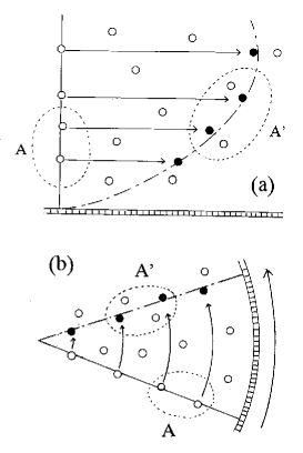
Figure 4: Two types of flows just above $T_{\lambda}$. Areas enclosed by a dotted line represent large but not yet macroscopic size of coherent wave functions, a size of which is exaggerated for clarity.

From our viewpoint, a remarkable state of the boson system lies at the vicinity of $T_{\lambda}$ in the normal phase ($\mu-\Sigma\leq 0$). In Fig.4, the coherent many-body wave function grows to a large but not yet a macroscopic size. (Approximately, the chemical potential $\mu$, hence $\mu-\Sigma$ as well, is inversely proportional to the size of the coherent many-body wave function mat , which corresponds to the size of regions enclosed by a dotted line in Fig.4.) The permutation symmetry holds only within each of these regions. When particles are moved from a region A to another region A’ in Fig.4(a), the mechanism below $T_{\lambda}$ does not work. But the repulsive interaction $U$, not only determining $\nu_{n}$ in Eq.(27), but also affects the role of Bose statistics as follows. In general, when a particle moves in the interacting system, it induces the motions of other particles. In particular, the long-distance displacement of a particle in coordinate space causes the excitation of many particles, and therefore it needs a high excitation energy. Hence, the short-distance displacement is a major ingredient of the low-energy excitation. This means that excited particles are not likely to go beyond a single coherent wave function, but likely to remain in it. Hence, under the repulsive interaction, the suppression mechanism of the low-energy excitation owing to Bose statistics works just above $T_{\lambda}$ as well. (A similar argument holds in the rotational flow in Fig.4(b) koh .)

This interplay between Bose statistics and the repulsive interaction will appear as follows. If we increase the strength of $U$, the excited bosons get to remain in the same coherent wave function, and therefore the low-energy transverse excitation will raises its energy. The relaxation time to the ground state becomes short, thus making the shear viscosity fall off. In Eq.(26), the condition of $\chi^{L}(q,0)=\chi^{T}(q,0)$ at $q\rightarrow 0$ will be violated at a certain critical value of $U$. In real materials, we realize this situation in an alternative manner. If we decrease the temperature at a given $U$, the coherent wave function obeying Bose statistics grows. The above condition will be violated at a certain temperature , which will give the onset temperature of the decease of $\eta$ in Fig.1(a).

III Susceptibility and shear viscosity above $T_{\lambda}$

Let us formulate the influence of Bose statistics on the shear viscosity. Equation (26) says that $\chi^{L}(q,\omega)-\chi^{T}(q,\omega)$ is a crucial quantity for this purpose. The problem is how to formulate in this quantity the interplay between Bose statistics and the repulsive interaction. Under the repulsive interaction $\hat{H_{I}}(\tau)$, one considers the integrand of Eq.(17) as

$$<G|T_{\tau}J_{\mu}(x,\tau)J_{\nu}(0,0)|G>=\frac{\displaystyle{<0|T_{\tau}\hat{J}_{\mu}(x,\tau)\hat{J}_{\nu}(0,0)exp\left[-\int_{0}^{\beta}d\tau\hat{H}_{I}(\tau)\right]|0>}}{\displaystyle{<0|exp\left[-\int_{0}^{\beta}d\tau\hat{H}_{I}(\tau)\right]|0>}}.$$ (31)

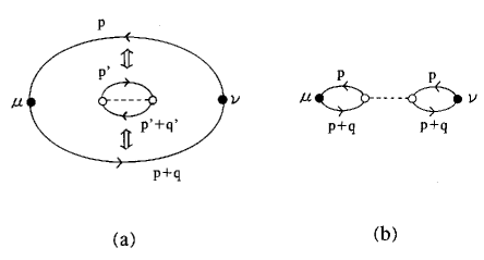
Figure 5: The process of line exchanges due to Bose statistics occurring in $J_{\mu}J_{\nu}exp[-\int d\tau H_{I}(\tau)]$ of Eq.(31). Two times of the line exchange in Fig.5(a), between a current-current response tensor $J_{\mu}J_{\nu}$ (a large bubble) and a bubble excitation by the repulsive interaction $U$ (an inner small bubble with a dotted line), yields Fig.5(b). (The black and white small circle represents a vector and scalar vertex, respectively.)

Figure 5(a) illustrates the current-current response tensor $\hat{J}_{\mu}(x,\tau)\hat{J}_{\nu}(0,0)$ (a large bubble with $\mu$ and $\nu$) in the medium: Owing to $exp(-\smallint\hat{H}_{I}(\tau)d\tau)$ in Eq.(31), scatterings of particles frequently occur in $|G>$ as illustrated by an inner small bubble with a dotted line $U$. (The black and white circle represents a coupling to $\mbox{\boldmath$v$}_{d}(\mbox{\boldmath$q$})$ and $U$, respectively.) The state $|G>$ includes many interaction bubbles like the small one with various momentums $p^{\prime}$ and $p^{\prime}+q^{\prime}$. A solid line with an arrow represents

$$G(i\omega_{n},p)=\frac{1}{i\omega_{n}-\epsilon(p)-\Sigma+\mu}.$$ (32)

($\mu$ is a chemical potential implicitly determined by $V^{-1}\Sigma[\exp(\beta[\epsilon(q)+\Sigma-\mu])-1]^{-1}=n$). Owing to the repulsive interaction, the boson has a self energy $\Sigma$ ($>0$) (we ignore its $\omega$ and $p$ dependence by assuming it small). With decreasing temperature, the negative $\mu$ at high temperature approaches a small positive value of $\Sigma$, finally reaching Bose-Einstein condensation satisfying $\mu=\Sigma$.

When the system is just above $T_{\lambda}$ in the normal phase, particles in the ground state $|G>$ experience the strong influence of Bose statistics. Hence, the perturbation of $\hat{J}_{\mu}(x,\tau)\hat{J}_{\nu}(0,0)$ in Eq.(31) must be developed in such a way that, as the order of the perturbation increases, it gradually include a new effect due to Bose statistics. Specifically, the large bubble $\hat{J}_{\mu}(x,\tau)\hat{J}_{\nu}(0,0)$ and the small bubble in Fig.5(a) form a coherent wave function as a whole. When one of the two particles in the large bubble and in the small bubble have the same momentum ($p=p^{\prime}$), and the other in both bubbles have another same momentum ($p+q=p^{\prime}+q^{\prime}$) in Fig.5(a), a graph made by exchanging these particle lines must be included in the expansion. The exchange of two lines having $p$ and $p^{\prime}$($=p$), and the exchange of the other two lines having $p+q$ and $p+q^{\prime}$($=p+q$) yield Fig.5(b). The result is that two bubbles with the same momentums are linked by the repulsive interaction, yielding the following contribution to $\chi_{\mu\nu}(q,\omega)$

$$U\frac{1}{V}\sum_{p}(p+\frac{q}{2})_{\mu}(p+\frac{q}{2})_{\nu}\left[-\frac{f(\epsilon(p)+\Sigma)-f(\epsilon(p+q)+\Sigma)}{\omega+\epsilon(p)-\epsilon(p+q)}\right]^{2}.$$ (33)

(a) With decreasing temperature, the coherent wave function grows to a large size, and the exchange of particle lines owing to Bose statistics like Fig.5 occurs many times. Hence, one cannot ignore the higher-order terms in Eq.(31), which become more significant with the growth of the coherent wave function. Continuing these exchanges, one obtains the $l$-th order term which has two vector vertex (black circles) at both ends, to which $(p+\frac{q}{2})_{\mu}(p+\frac{q}{2})_{\nu}$ is attached, and $2l$ scalar vertex (white circles) between the two ends.

(b) Among physical processes in Eq.(33), it becomes evident with decreasing temperature that a process including zero momentum particles plays a dominant role. Specifically, a process with $p=0$ corresponds to an excitation from the rest particle, and a process with $p=-q$ corresponds to a decay into the rest one. These processes are important in the higher-order terms as well.

With these considerations (a) and (b), we obtain the following form of $\hat{\chi}_{\mu\nu}(q,0)=[\chi^{L}(q,0)-\chi^{T}(q,0)]q_{\mu}q_{\nu}/q^{2}$ at the vicinity of $T_{\lambda}$

$$\hat{\chi}_{\mu\nu}(q,0)=\frac{q_{\mu}q_{\nu}}{2}\frac{1}{V}\sum_{l=0}^{\infty}U^{l}F_{\beta}(q)^{l+1},$$ (34)

where

$$F_{\beta}(q)=\frac{(\exp(\beta[\Sigma-\mu]-1))^{-1}-(\exp(\beta[\epsilon(q)+\Sigma-\mu])-1)^{-1}}{\epsilon(q)}$$ (35)

is a positive monotonously decreasing function of $q^{2}$, which approaches zero as $q^{2}\rightarrow\infty$.

At a high temperature ($\beta\mu\ll 0$), $F_{\beta}(q)$ is small, and it guarantees the convergence of an infinite series in Eq.(34), with a result that

$$\hat{\chi}_{\mu\nu}(q,0)=\frac{q_{\mu}q_{\nu}}{2}\frac{1}{V}\frac{F_{\beta}(q)}{1-UF_{\beta}(q)}.$$ (36)

With decreasing temperature, however, the negative $\mu$ gradually approaches $\Sigma$, hence $\Sigma-\mu\rightarrow 0$. Since $F_{\beta}(q)$ increases as $\Sigma-\mu\rightarrow 0$, it makes the higher-order term significant in Eq.(34). Since $F_{\beta}(q)$ is a positive decreasing function of $q^{2}$, the divergence of Eq.(36) first occurs at $q^{2}=0$. An expansion of $F_{\beta}(q)$ around $q^{2}=0$, $F_{\beta}(0)-bq^{2}+\cdots$ has a form such as

$$F_{\beta}(q)=\frac{\beta}{4\sinh^{2}\displaystyle{\left(\frac{|\beta[\mu(T)-\Sigma]}{2}\right)}}\left[1-\frac{\beta}{2}\frac{1}{\tanh\displaystyle{\left(\frac{|\beta[\mu(T)-\Sigma]|}{2}\right)}}\frac{q^{2}}{2m}+\cdots\right].$$ (37)

At $q\rightarrow 0$, the denominator $1-UF_{\beta}(q)$ in the right-hand side of Eq.(36) has a form of $[1-UF_{\beta}(0)]+Ubq^{2}$. With decreasing temperature ($\Sigma-\mu\rightarrow 0$), $UF_{\beta}(0)$ increases and finally reaches 1, that is,

$$U\beta=4\sinh^{2}\left(\frac{\beta[\mu(T)-\Sigma(U)]}{2}\right).$$ (38)

At this point, the denominator in Eq.(36) gets to begin with $q^{2}$, and $\hat{\chi}_{\mu\nu}(q,0)$ therefore changes to have a form of $q_{\mu}q_{\nu}/q^{2}$ at $q\rightarrow 0$, and $q_{\mu}q_{\nu}/q^{2}$ has a non-zero coefficient $F_{\beta}(0)/(2VUb)$. In view of the definition of Eq.(19), this result implies $\lim_{q\to 0}[\chi^{L}(q,0)-\chi^{T}(q,0)]\neq 0$ in Eq.(26). From now, we call $T$ satisfying Eq.(38) the onset temperature $T_{on}$ com .

At $T=T_{on}$, substituting Eq.(37) into Eq.(36), we obtain $\hat{\chi}_{\mu\nu}$ at $q\rightarrow 0$

$$\hat{\chi}_{\mu\nu}(q,0)=\frac{2m}{U\beta_{on}}\frac{1}{V}\tanh\left(\frac{|\beta_{on}[\mu(T_{on})-\Sigma]|}{2}\right)\frac{q_{\mu}q_{\nu}}{q^{2}}.$$ (39)

By the definition of $\hat{\rho_{s}}(T)=\lim_{q\to 0}(q^{2}/q_{\mu}q_{\nu})\hat{\chi}_{\mu\nu}$, one obtains with the aid of Eq.(38)

$$\hat{\rho_{s}}(T_{on})=\frac{1}{V}\frac{m}{\sinh|\beta_{on}[\mu(T_{on})-\Sigma]|}.$$ (40)

The mechanical superfluid density $\hat{\rho_{s}}(T)$ is given by $mc(T)n_{0}(T)$, where

$$c(T)=\frac{2}{\exp(\beta|\mu(T)-\Sigma|)+1}$$ (41)

is a Fermi-distribution-like coefficient, and

$$n_{0}(T)=\frac{1}{V}\frac{1}{\exp(-\beta[\mu(T)-\Sigma])-1}$$ (42)

is the number density of $p=0$ bosons. In the $V\rightarrow\infty$ limit, this quantity is normally regarded to be zero. For the finite system just above $T_{\lambda}$, however, $n_{0}(T)$ has a large but not yet macroscopic value. In real finite system, its magnitude must be estimated by experiments (see Sec.4).

The violation of $\chi^{T}(q,0)=\chi^{L}(q,0)$ at $q\rightarrow 0$ gives rise to various anomalous mechanical responses of a superfluid. At the vicinity of $T_{\lambda}$, Eq.(38) is approximated as $U\beta=\beta^{2}[\mu(T)-\Sigma(U)]^{2}$ for a small $\mu-\Sigma$. This condition has two solutions $\mu(T)=\Sigma(U)\pm\sqrt{Uk_{B}T}$. It is generally assumed that the repulsive Bose system undergoes BEC as well as a free Bose gas. Hence, with decreasing temperature, $\mu(T)$ of repulsive Bose system should reach $\Sigma(U)$ at a finite temperature, during which course the system necessarily passes a state satisfying $\mu(T)=\Sigma(U)-\sqrt{Uk_{B}T}$. Consequently, the anomalous mechanical response of a superfluid appears prior to $T_{\lambda}$. Using Eq.(40) in the formula of the kinematic shear viscosity (Eq.(27)), we obtain $\nu(T)$ at the vicinity of $T_{\lambda}$, which always falls off prior to BEC , that is, $T_{on}>T_{\lambda}$. Among various mechanical responses of a liquid helium 4 above $T_{\lambda}$, the shear viscosity coefficient most evidently shows a change toward superfluidity far above the critical region. This feature comes from the structure of Eq.(27), in which the small $\omega_{s}$ amplifies a small $\hat{\rho_{s}}(T)/\rho$ to an observable change of $\nu(T)$.

The phenomenon at $T_{on}$ has the following difference from thermal fluctuations. Since the thermal fluctuation is essentially a local phenomenon, its influence already appears in the low-order terms of the perturbation expansion in which only a few particles participate. In Eq.(34), however, only after the perturbation expansion is summed up to the infinite order, the non-zero $\hat{\rho_{s}}(T)$ defined as $\lim_{q\to 0}[q^{2}/(q_{\mu}q_{\nu})]\hat{\chi}_{\mu\nu}$ appears lod pha .

With decreasing temperature from $T_{on}$, in addition to the particle with $p=0$, other particles having small but finite momentums get to contribute to the $1/q^{2}$ divergence of $\hat{\chi}_{\mu\nu}(q,0)$ as well. (In addition to Eq.(35), a new $F_{\beta}(q)$ including $p\neq 0$ also satisfies $1-UF_{\beta}(0)=0$ in Eq.(36).) Hence, the mechanical superfluid density increases. On this change, we have the following physical explanation. For the repulsive Bose system, particles are likely to spread uniformly in coordinate space due to the repulsive force. This feature makes the particles with $p\neq 0$ behave similarly with other particles, especially with the particle having zero momentum. If they behave differently from others, a resulting locally high density of particle raises the interaction energy. This is a reason why many particles participate in the singular dynamical behavior even at a temperature in which only a few particles participate in the coherent many-body wave function . In contrast with the thermodynamical superfluid density $\rho_{s}(T)$, the mechanical superfluid density $\hat{\rho_{s}}(T)$ is a concept including such a dynamics of the system.

When the system reaches $T=T_{\lambda}$ in which $\mu=\Sigma$ is satisfied, one notes $c(T_{\lambda})=1$ and $n_{0}(T_{\lambda})=n_{c}$. This means that the zero momentum part of $\hat{\rho_{s}}(T_{\lambda})$ agrees with the conventional thermodynamical superfluid density $\rho_{s}(T_{\lambda})=mn_{c}$, and $n_{c}$ abruptly grows to a macroscopic number. While $\hat{\rho_{s}}(T)$ at $T>T_{\lambda}$ vanishes in the $V\rightarrow\infty$ limit, $\hat{\rho_{s}}(T)$ at $T<T_{\lambda}$ remains finite in this limit. Hence, in thermodynamics, only the latter remains. In the mechanical response of the finite system, however, $\hat{\rho_{s}}(T)$ manifests itself already at $T>T_{\lambda}$.

IV Comparison to experiments

At $T>2.8K$ in 1 atm, the shear viscosity of a liquid helium 4 slightly increases with decreasing temperature. As shown in Fig.1(a), after reaching a maximum value at 2.8K, it begins to reduce its value. On the contrary, the shear viscosity of a classical liquid has the general property of increasing monotonously with decreasing temperature she . At first sight, a liquid helium 4 seems to undergo a crossover from a classical to a quantum liquid at 2.8K, but it is superficial. Comparing Eq.(26) and (27), one notes that $\nu(T)$ is a more appropriate quantity than $\eta(T)$ for describing simply the change of the system around $T_{\lambda}$. As shown in Fig.6(a), the total density $\rho(T)$ of a liquid helium 4 in the normal phase monotonously increases with decreasing temperature until $T=T_{\lambda}$ den . Fig.6(b) shows the kinematic shear viscosity $\nu(T)=\eta(T)/\rho(T)$ using $\eta(T)$ (Fig.1(a)) and $\rho(T)$ (Fig.6(a)), revealing that $\nu(T)$ monotonously decreases with decreasing temperature over the whole range of $T_{\lambda}<T<4.2K$. This means that in 1 atm, it is just below the gas-liquid condensation point $T_{c}=4.2K$ that the strong influence of Bose statistics begins to suppress the shear viscosity in a liquid helium 4.

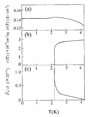
Figure 6: (a) The temperature dependence of the total density $\rho$ of a liquid helium 4 (after the data in Ref.34). (b) The temperature dependence of the kinematic shear viscosity $\nu$ of a liquid helium 4 obtained using Fig.1(a) and Fig.6(a). (c) $\hat{\rho}_{s}(T)/\rho$ obtained by Eq.(43) using $\nu(T)$ in Fig.6(b) and $\omega_{s}=5\times 10^{-3}rad/s$.

This temperature dependence and the smallness of $\nu(T)$ implies that a liquid helium 4 in the normal phase is already an anomalous liquid under the strong influence of Bose statistics. In a strict sense, it is not certain whether there is a completely classical regime in liquid helium 4 at 1 atm. But, even if we assume $T_{on}>4.2K$, it is impossible to analyze the onset mechanism of the decrease of $\nu$ in a virtual liquid at $T>4.2K$ in 1 atm. For the present, we assume $T_{on}=4.2K$, and interpret $\nu(T)$ in Fig.6(b) using Eq.(27) with $\nu_{n}=\nu(T_{on})$. One obtains $\hat{\rho}_{s}(T)/\rho$ by

$$\frac{8}{\pi a^{2}\omega_{s}}\frac{\hat{\rho}_{s}(T)}{\rho}=\nu(T)^{-1}-\nu(T_{on})^{-1}.$$ (43)

A typical value of the capillary radius used in the experiment in Ref.3, 4 and 5 is $a\simeq 5\times 10^{-3}cm$. In the rotation experiment by Hess and Fairbank hes , the moment of inertia $I_{z}$ just above $T_{\lambda}$ is slightly smaller than the normal phase value $I_{z}^{cl}$ (see Sec.5.B). Using these data, Ref.14 roughly estimates $\hat{\rho_{s}}(T_{\lambda}+0.03K)/\rho\cong 8\times 10^{-5}$, and $\hat{\rho_{s}}(T_{\lambda}+0.28K)/\rho\cong 3\times 10^{-5}$. With these values and $\nu(T)$ in Fig.6(b), we obtain a rough estimation of $\omega_{s}$ as $\omega_{s}\simeq 5\times 10^{-3}rad/s$ at these two temperatures just above $T_{\lambda}$. Figure 6(c) shows a resulting temperature dependence of $\hat{\rho}_{s}(T)/\rho$. (Since the precision of these two values of $\hat{\rho}_{s}(T)/\rho$ derived from currently available data is limited, the absolute value of $\hat{\rho}_{s}(T)/\rho$ in Fig.6(c) has a statistical uncertainty.)

The quantity which directly indicates the onset of superfluidity in dissipative system is the change of the conductivity spectrum $\sigma(\omega)$. In view of the gradual decrease of $\eta$ above $T_{\lambda}$, the sharp peak around $\omega=0$ and the corresponding change from $\sigma(\omega)$ to $\sigma_{n}(\omega)$ in Fig.3 must already appear at $T>T_{\lambda}$. (Since this change does not occur in the case of thermal fluctuations, it is useful for ruling out the possibility of fluctuations.) To confirm this prediction, the time-resolved measurement of the oscillating flow velocity $\mbox{\boldmath$v$}(\mbox{\boldmath$r$},t)$ is necessary under the slowly oscillating pressure gradient. Such an experiment must be performed in a thin capillary with an inner radius of $10^{-2}\sim 10^{-1}$ mm. Recently, the PIV technique recorded the velocity of tracer particles in a flow of liquid helium 4, and mapped out the velocity field $\mbox{\boldmath$v$}(\mbox{\boldmath$r$})$ in a pipe don van . If the PIV experiment is performed under the above conditions, the change of $\sigma(\omega)$ in Fig.3 will be observed. There is now ambiguity in interpretation of the movement of tracer particles poo . If tracer particles interact only with the normal fluid flow and trace its velocity, the change from $\sigma(\omega)$ to $\sigma_{n}(\omega)$ as in Fig.3 will be observed. The quantity $A$ in Eq.(10) is equal to the area of the shaded region $\sigma(\omega)-\sigma_{n}(\omega)$ in Fig.3(b). On the other hand, if tracer particles interact with the superfluid flow as well, the emergence of the sharp peak around $\omega=0$ as in Fig.(b) will be detected. In any case, using thus obtained $A$, one can determine $\omega_{s}$ by interpreting the experimental data of $\eta(T)$ with Eq.(10). Furthermore, using $A=2\hat{\rho}_{s}(T)/(\pi a^{2})$, one will obtain an independent estimate of $\hat{\rho}_{s}(T)/\rho$ at $T>T_{\lambda}$. Although such an experiment may be a difficult one, it is an experiment worth attempting.

V Discussion

V.1 Interpretation of the $\lambda$-shape of specific heat

Bose-Einstein condensation differs from ordinary phase transitions in that it occurs without interactions between particles. At the early stages in the history of the study of phase-transition in the early part of twentieth century, almost all phase transitions were thought to have a $\lambda$-like-shaped temperature dependence of the specific heat $C(T)$ at the vicinity of $T_{c}$. As the precision of experiments was improved, however, it became clear that $C(T)$ in most phase transitions has, not the $\lambda$-like shape, but a $\delta$-function-like one. In a liquid helium 4, however, the precise measurements revealed that $C(T)$ intrinsically has the $\lambda$-like temperature dependence. The principal peak at $T_{\lambda}$ has been a subject of intensive studies of the critical phenomena. Furthermore, the gradual rise of $C(T)$ above $T_{\lambda}$ has been interpreted as a sign of enhanced thermal fluctuations specific to the Bose systems near $T_{\lambda}$.

There is a reason that such a fluctuation-based interpretation was accepted on the gradual rise of $C(T)$. In theories of the Bose system, the $V\rightarrow\infty$ limit is normally used. In this limit, the number density of particles with zero momentum is exactly zero at $T>T_{\lambda}$, and is finite only at $T\leq T_{\lambda}$. (In the equation of states $N/V=g_{3/2}(e^{\beta\mu})+V^{-1}e^{\beta\mu}/(1-e^{\beta\mu})$ where $g_{a}(x)=\sum_{n}x^{n}/n^{a}$, the zero momentum part $V^{-1}e^{\beta\mu}/(1-e^{\beta\mu})$ has a finite value at $V\rightarrow\infty$ limit only when $e^{\beta\mu}/(1-e^{\beta\mu})$ diverges, that is, $\mu=0$.) The $V\rightarrow\infty$ limit is necessary for the definition of the phase transition that the thermal average of the order parameter is exactly zero above $T_{c}$.

The $V\rightarrow\infty$ limit is a good approximation only when one can clearly distinguish between microscopic and macroscopic phenomena. In the Bose system, however, the distinction between “microscopic” and “macroscopic” is not so obvious as in other phenomena. Since particles with zero momentum plays an important role at low temperature, the coherent many-body wave function with a macroscopic wave length plays a significant role in microscopic descriptions of the system. In this sense, “microscopic” and “macroscopic” coexist from the beginning. But, if we naively apply this $V\rightarrow\infty$ limit to the anomalous response at $T>T_{\lambda}$, the thermal average of the output quantity is set to be zero by $V\rightarrow\infty$, and we are forced to regard all of them as being caused by thermal fluctuations. We must carefully examine the validity of regarding a whole sample as occupying an infinite volume. In the thermodynamical viewpoint using $V\rightarrow\infty$, the intermediate-sized coherent wave function plays a minor role above $T_{\lambda}$, but for the Bose system above $T_{\lambda}$, it substantially affects the system. Hence, we must experimentally estimate the magnitude of effects hidden by this $V\rightarrow\infty$ limit. In this paper, we viewed the gradual decrease of $\eta$ above $T_{\lambda}$ from this point vie , and showed that the growth of the intermediate-sized coherent wave function gives rise to the decrease of $\eta$ .

V.2 Superfluidity in the dissipative and the non-dissipative systems

As an example of the non-dissipative systems, we considered a rotational flow. In the rotational flow, the quantity directly indicating the onset of superfluidity is the moment of inertia

$$I_{z}=I_{z}^{cl}\left(1-\frac{\hat{\rho_{s}}(T)}{\rho}\right),$$ (44)

where $I_{z}^{cl}$ is its classical value koh . On the onset mechanism of superfluidity, one can see the physical difference between the dissipative and the non-dissipative systems in Eq.(27) and (44).

(a) In Eq.(44), $\hat{\rho_{s}}(T)$ appears as a correction to the coefficient of the linear term of $I_{z}^{cl}$. On the other hand, in the expansion of Eq.(27) with respect to $\nu_{n}$, $\hat{\rho_{s}}(T)$ appears in the non-linear higher-order terms of $\nu_{n}$. Furthermore, with decreasing temperature, the higher-order terms become dominant in Eq.(27).

(b) In Eq.(44), the change of the transverse excitations appears in $I_{z}$ without being enhanced, and therefore the nonzero $\hat{\rho_{s}}(T)$ only slightly affects $I_{z}$ above $T_{\lambda}$. On the other hand, in Eq.(27), the change of the transverse excitations does not directly appear in $\nu$, but through the dispersion integral as in Eq.(23), which is a characteristic feature of the dissipative systems. During this process, a sign of superfluidity in the dissipative systems is enhanced to an observable scale.

(c) In Eq.(27), the peak width $\omega_{s}$ reflects a degree of the rigidity of superfluidity, which is derived from the $\omega$ dependence of $\lim_{q\to 0}[\chi^{L}(q,\omega)-\chi^{T}(q,\omega)]$, whereas $\omega_{s}$ does not appear in Eq.(44). This feature is characteristic to superfluidity in the dissipative systems, which manifests itself while showing the rigidity against the dissipation. The microscopic derivation of $\omega_{s}$ is a future problem.

In principle, it is possible to begin with Eq.(5), and obtain Eq.(27) after perturbation calculations. But it may require a knowledge of the dissipation mechanism in a liquid. In other words, the correct model of the dissipation mechanism of a liquid must reproduce Eq.(27) on the influence of superfluidity, because Eq.(27) is based on the general argument. In this sense, one can use this requirement as a criterion of the correct model of a liquid.

As another example of superfluidity in the dissipative system, one knows the anomalous thermal conductivity of a liquid helium 4 at $T<T_{\lambda}$. Heat flow $q$ is expressed as $q=-\kappa\nabla T$, where $\kappa$ is the thermal conductivity coefficient. At $T=T_{\lambda}$, $\kappa$ jumps to a $10^{7}$ times larger value than $\kappa$ just above $T_{\lambda}$. At $T_{\lambda}<T<2.8K$, however, the gradual rise of $\kappa$ corresponding to the gradual fall of $\eta$ is not observed kel . Formally, we do not know a non-dissipative phenomenon complementary to the heat conduction, like the rotational flow in the shear viscosity. Hence, we can not apply the formalism in this paper to the onset mechanism of the anomalous thermal conductivity. This difference between heat conduction and shear viscosity on a formal level may have some implication on the absence of the gradual rise of $\kappa$ at $T_{\lambda}<T<2.8K$.

V.3 Comparison to Fermi liquids

In a liquid helium 3, the fall of the shear viscosity at $T_{c}$ is known as a parallel phenomenon to that of a liquid helium 4. The formalism in Sec.2 is also applicable to the shear viscosity of a liquid helium 3. For the behavior above $T_{c}$, however, there is a striking difference between a liquid helium 3 and 4. The phenomenon occurring in fermions at the vicinity of $T_{c}$ is not a gradual growth of the coherent wave function, but a formation of the Cooper pairs from two fermions. (This difference evidently appears in the temperature dependence of the specific heat: $C(T)$ of a liquid helium 3 just above $T_{c}$ does not show the symptom of its rise to the sharp peak.) Once the Cooper pairs are formed, they are composite bosons situated at low temperature and high density, and immediately jumps to the ESP or BW state. Hence, the shear viscosity of a liquid helium 3 shows an abrupt drop at $T_{c}$ without a gradual fall above $T_{c}$.

In electron superconductivity, the fluctuation-enhanced conductivity $\sigma^{\prime}$ is observed above $T_{c}$ ttin . In bulk superconductors, however, the ratio of $\sigma^{\prime}$ to the normal conductivity $\sigma_{n}$ is about $10^{-5}$ at the critical region, and zero outside of this region. Practically, it is unlikely that thermal fluctuations create a large change of $\sigma$ at temperatures outside of the critical region.

Appendix A Maxwell’s relation

Consider the shear transformation of a solid and of a liquid. In a solid, the shear stress $F_{xy}$ is proportional to a shear angle $\phi$ as $F_{xy}=G\phi$, where $G$ is the modulus of rigidity. The value of $G$ is determined by dynamical processes in which vacancies in a solid move to neighboring positions over the energy barriers. As $\phi$ increases, $F_{xy}$ increases as follows,

$$\frac{dF_{xy}}{dt}=G\frac{d\phi}{dt}.$$ (45)

In a liquid, the flow motion rearranges the relative position of particles, reducing the shear stress $F_{xy}$ to a certain value. Presumably, the rate of such a relaxation is proportional to the magnitude of $F_{xy}$, and one obtains

$$\frac{dF_{xy}}{dt}=G\frac{d\phi}{dt}-\frac{F_{xy}}{\tau}.$$ (46)

In the stationary flow after relaxation, $F_{xy}$ remains constant, and one obtains

$$G\frac{d\phi}{dt}=\frac{F_{xy}}{\tau}.$$ (47)

Figure.7 shows two particles 1 and 2, each of which starts at $(x,y)$ and $(x,y+\Delta y)$ simultaneously and moving along the $x$-direction. Consider a velocity gradient $v_{x}(y)$ along $y$ direction. After $\Delta t$ has passed, they (1’ and 2’) are at a distance of $\Delta v_{x}\Delta t$ along the $x$-direction. As a result, the shear angle increases from zero to $\Delta\phi$, which satisfies $\Delta v_{x}\Delta t=\Delta y\Delta\phi$ as depicted in Fig.7. Hence, we obtain

$$\frac{\partial v_{x}}{\partial y}=\frac{d\phi}{dt}.$$ (48)

Using Eq.(A4) in Eq.(A3), and comparing it with Eq.(1), one obtains $\eta=G\tau$ (Maxwell’s relation).

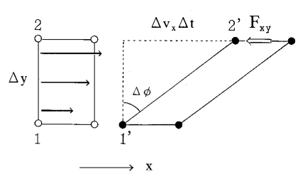
Figure 7: In a liquid flowing along the $x$-direction, owing to the velocity gradient along the $y$-direction, a small part of a liquid with a rectangular shape transforms to a shape whose cross section is a parallelogram.

Appendix B Conductivity spectrum $\sigma(\omega)$

The Navier-Stokes equation under the oscillating pressure gradient $\Delta Pe^{i\omega t}/L$ is written in the cylindrical polar coordinate as follows

$$\frac{\partial v}{\partial t}=\nu\left(\frac{\partial}{\partial r^{2}}+\frac{\partial}{r\partial r}\right)v+\frac{\Delta Pe^{i\omega t}}{\rho L}.$$ (49)

The velocity field has the following form

$$v(r,t)=\frac{\Delta Pe^{i\omega t}}{i\omega\rho L}+\Delta v(r,t),$$ (50)

with the boundary condition of $v(a,t)=0$. $\Delta v(r,t)$ satisfies

$$\frac{\partial\Delta v(r,t)}{\partial t}=\nu\left(\frac{\partial}{\partial r^{2}}+\frac{\partial}{r\partial r}\right)\Delta v(r,t),$$ (51)

and therefore $\Delta v(r,t)$ has a form of Bessel function $J_{0}(i\lambda r)$ with $\lambda=(1+i)\sqrt{\omega/(2\nu)}$. Hence,

$$v(r,t)=\frac{\Delta Pe^{i\omega t}}{i\omega\rho L}\left(1-\frac{J_{0}(i\lambda r)}{J_{0}(i\lambda a)}\right).$$ (52)

At $r=0$, the conductivity $\sigma(\omega)$ satisfying $\rho v(0,t)=\sigma(\omega)a^{2}\Delta Pe^{i\omega t}/L$ is given by

$$\sigma(\omega)=\frac{1}{i\omega a^{2}}\left(1-\frac{1}{J_{0}(ia(1+i)\displaystyle{\sqrt{\frac{\omega}{2\nu}}})}\right).$$ (53)

Re $\sigma(\omega)$ is schematically illustrated in Fig.3(a). (Re $\sigma(0)$ in Eq.(B5) agrees with Eq.(6). Im $\sigma(\omega)$ gives an expression of $\sigma_{2}(\omega)$ in Eq.(11), but it does not agree with $\sigma_{2}(0,\omega)$ in Eq.(20), because it is derived from the phenomenological equation with dissipation like the Navier-Stokes equation.)

References

- (1) P.Kapitza, Nature,141, 74(1938), J.F.Allen and A.D.Meissner, Nature,141, 75(1938)
- (2) L.D.Landau and I.M. Khalatonikov, Zh.Eksp.Teor.Fiz,19, 637, 709(1949), in Collected papers of L.D.Landau, (edited by D.ter.Haar, Pergamon, London, 1965).
- (3) R.Bowers and K.Mendelssohn, Proc.Roy.Soc.Lond.A,204, 366(1950)
- (4) H.Tjerkstra, Physica, 19, 217(1953)
- (5) K.N.Zinoveva, Zh.Eksp.Teor.Fiz,34, 609(1958) [Sov.Phys-JETP,7, 421(1958)]
- (6) J.C.Maxwell, Phil.Trans.Roy.Soc,157, 49(1867) in The scientific papers of J.C.Maxwell, (edited by W.D.Niven, Dover, New York, 2003) Vol.2, 26.
- (7) As a text, J.P.Hansen and I.R.McDonald, Theory of Simple Liquids, 3rd ed, (Academic Press, London, 2006).
- (8) R.A.Ferrell and R.E.Glover, Phy.Rev,109, 1398(1958), M.Tinkham and R.A.Ferrell, Phy.Rev,2, 331(1959)
- (9) As a text, M.Tinkham Introduction to superconductivity, 2nd ed, (McGraw-Hill, New York, 1996).
- (10) As a review, P.Nozieres, in Quantum Fluids (ed by D.E.Brewer), 1 (North Holland, Amsterdam, 1966), G.Baym, in Mathematical methods in Solid State and Superfluid Theory (ed by R.C.Clark and G.H.Derrick), 121 (Oliver and Boyd, Edingburgh, 1969)
- (11) The principal peak in corresponds to the sharp drop in at . In this region, the measurement shows (G.Ahlers, Phys.Let.A 37, 151 (1971)). The critical exponent was studied in the context of the dynamical critical phenomena in A.M.Polyakov, Zh.Eksp.Teor.Fiz.57, 2144(1969), [Sov.Phys.JETP.30, 1164(1970)].
- (12) London stressed that the essence of superfluidity is not the absence of the viscosity, but the occurrence of in F.London Superfluid, (John Wiely and Sons, New York, 1954) Vol.2, 141. Although this remark is essentially correct, it does not rule out the possibility that behind the substantial decrease of in a liquid helium 4 above , the condition of is locally realized by the intermediate-sized coherent wave function. Since is a spatial order extending to many particles, it is impossible for the short-lived random fluctuations to create it.
- (13) The following derivations of the transition intuitively illustrates this continuous change of the system. T.Matsubara, Prog.Theo.Phys.6, 714 (1951), and R.P.Feynman, Phys.Rev. 90, 1116 (1953), ibid 91, 1291 (1953).
- (14) S.Koh, Phy.Rev.B.74, 054501(2006).
- (15) S.Koh, Phy.Rev.B.68, 144502(2003).
- (16) R.J.Donnelly,A.N.Karpetis, J.J.Niemela, K.R.Sreenivasan, W.F.Vinen and C.M.White, J.Low.Temp.Phys. 126, 327(2002),
- (17) T.Zhang, D.Celik and S.W.Van Sciver, J.Low.Temp.Phys. 134, 985(2004), T.Zhang and S.W.Van Sciver, J.Low.Temp.Phys. 138, 865(2005)
- (18) L.P.Kadanoff and P.C.Martin, Ann.Phys. 24, 419(1963), P.C.Hoenberg and P.C.Martin, Ann.Phys. 34, 291(1965).
- (19) The one-loop term in the perturbation expansion of Eq.(5) reproduces the formula in the kinetic theory of gases. Beyond the one-loop level, the shear viscosity of model is calculated in the context of the relativistic heavy ion collision by S.Jeon, Phy.Rev.D,52, 3591(1995), E.Wang and U.Heinz, Phys.Lett.B, 52, 208(1999). These results describe the shear viscosity of a strongly interacting dense gas. For a liquid, however, the anisotropic particle interaction with the hard core must be introduced in calculations.
- (20) As a response to , at another point in a flow is possible, but it results in the same form of .
- (21) Equation (8) is the oscillator-strength sum rule in terms of the conductivity.
- (22) The particle density is adjusted to 1. In Ref.8, the definition of the vector potential plays the same role as Eq.(14).
- (23) In the fluctuation theory, the correlation function of deviations from a mean value gives a susceptibility around , an average of which is taken with the Gauss distribution. Owing to the flatness of the minimum of the thermodynamic potential near , the susceptibility has dependence. On the other hand, the susceptibility (Eq.(17) and (31)) is given as the correlation function of a total quantity . Its average is taken with the Bose-Einstein distribution. Hence, the result has no dependence.
- (24) Whatever complicated approximation is made for the susceptibility, the treatment in Eq.(19) enables us to easily derive the superfluid density from it.
- (25) Our ordinary use of as a longitudinal susceptibility satisfying , and the appearance of in the conductivity as a transverse response are made compatible by the fact that a replacement of by is possible in Eq.(21).
- (26) R.P.Feynman, in Progress in Low Temp Phys. 1, (ed C.J.Gorter), 17 (North-Holland, Amsterdam, 1955).
- (27) For the longitudinal displacement, the large-scale inhomogeneity occurs in the particle density, and it is therefore impossible to find, in the initial configuration, a particle close to that particle after displacement. See Fig.1 of Ref.15.
- (28) In an ordinary liquid, is determined by the individual motion of particles. Hence, it is not as small as of the collective relaxation by the coherent wave function in a superfluid.
- (29) G.B.Hess and W.M.Fairbank, Phy.Rev,19, 216(1967)
- (30) R.E.Packard and T.M.Sanders, Phy.Rev,6, 799(1972)
- (31) In addition to the bubble, it is possible that more complex diagrams, featuring intense excitations in a liquid, exchange particle lines with the tensor in Fig.5(a). While it is difficult to estimate an infinite sum of these diagrams, it adds only a small correction to the onset mechanism of the decrease of .
- (32) Thermal fluctuations occurring in the critical region of the point were examined in R.A.Farrell, N.Menyhard, H.Schmidt, F.Schwabl and P.Szepfalusy, Ann.Phys. 47, 565(1968). They considered the nonlocal superfluid density under the influence of the phase fluctuation of the order parameter. This quantity only slightly deviates from the conventional superfluid density within the range of , and is a different concept from .
- (33) of a classical liquid is inversely proportional to the rate of a process in which a vacancy in a liquid propagates from one point to another over the energy barriers. With decreasing temperature, this rate decreases, thus increasing .
- (34) E.C.Kerr, J.Chem.Phys, 26, 511(1957), and E.C.Kerr and R.D.Taylor, Ann.Phys. 26, 292(1964).
- (35) D.R.Poole, C.F.Barenghi, Y.A.Sergeev and W.F.Vinen, Phy.Rev. B71, 064514(2005).
- (36) The magnitude of the decrease of in a capillary flow around is strongly dependent on the radius of a capillary, suggesting that the distinction between “microscopic” and “macroscopic” is obscure, and exhibiting a feature of mesoscopic physics.
- (37) L.J.Challis and J.Wilks, in Proceedings of the Symposium on Solid and Liquid (Ohio State University, Ohio, 1957). J.F.Kerrisk and W.E.Keller, Phy.Rev,177, 341(1969).