Anisotropic surface reaction limited phase transformation dynamics in LiFePO₄

Abstract

A general continuum theory is developed for ion intercalation dynamics in a single crystal of a rechargeable battery cathode. It is based on an existing phase-field formulation of the bulk free energy and incorporates two crucial effects: (i) anisotropic ionic mobility in the crystal and (ii) surface reactions governing the flux of ions across the electrode/electrolyte interface, depending on the local free energy difference. Although the phase boundary can form a classical diffusive “shrinking core” when the dynamics is bulk-transport-limited, the theory also predicts a new regime of surface-reaction-limited (SRL) dynamics, where the phase boundary extends from surface to surface along planes of fast ionic diffusion, consistent with recent experiments on LiFePO₄. In the SRL regime, the theory produces a fundamentally new equation for phase transformation dynamics, which admits traveling-wave solutions. Rather than forming a shrinking core of untransformed material, the phase boundary advances by filling (or emptying) successive channels of fast diffusion in the crystal. By considering the random nucleation of SRL phase-transformation waves, the theory predicts a very different picture of charge/discharge dynamics from the classical diffusion-limited model, which could affect the interpretation of experimental data for LiFePO₄.

I Introduction

LiFePO₄ is widely considered to be a promising cathode material for Li-ion rechargeable batteries. The high practical capacity and reasonable operating voltage of the material, along with its nontoxicity and potential low cost, make it well-suited for large-scale battery applications Padhi et al. (1997); Yamada et al. (2001); Chung et al. (2002). Unlike many other cathode materials that increase their Li concentration in a continuous solid solution, Li_xFePO₄ only exists for $x\approx 0$ and $x\approx 1$ Delacourt et al. (2005) and charges or discharges Li by changing the fraction of phase with $x\approx 0$ and $x\approx 1$.

The transport and phase separation properties of LiFePO₄ have been studied extensively by atomistic simulations Morgan et al. (2004); Ouyang et al. (2004); Islam et al. (2005); Zhou et al. (2006). First-principles calculations have shown that Li diffusion in the bulk FePO₄ crystal is highly anisotropic Morgan et al. (2004); Ouyang et al. (2004). Li is essentially constrained to 1D channels in the (010) direction arranged in layers that form the crystal, as depicted in Fig. 1. The lattice mismatch at the FePO₄/LiFePO₄ phase boundary is significant (5% in the $x$ direction, shown in Fig. 1), and recent work has investigated the differences in elastic properties between the lithiated and unlithiated material Maxisch and Ceder (2006). Atomistic simulations have also suggested that electrons in the crystal may diffuse as small, localized polarons confined to planes parallel to the Li channels Xu et al. (2004); Zhou et al. (2004); Maxisch et al. (2006).

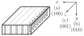
Figure 1: Schematic of plate-like single crystals of LiFePO₄. Li is confined to 1D channels in the $y$ direction, and channels are stacked in layers parallel to the $yz$ plane, indicated by the dotted lines. Typical dimensions of single crystals are $2\times 0.2\times 4$ $\mu$m in the $x$, $y$, $z$ dimensions, respectively Chen et al. (2006). For each direction, the corresponding space group Pnma axis and Miller index are shown in parentheses.

Recent experiments have confirmed the anisotropic transport and phase separation of Li in single crystal LiFePO₄ Chen et al. (2006); Laffont et al. (2006); Amin et al. (2007). Moreover, detailed microscopy in these studies has revealed that the FePO₄/LiFePO₄ phase boundary is a well-defined interface that extends through the bulk crystal to the surface. In experiments, the phase boundary has a characteristic width of several nanometers on the surface Laffont et al. (2006), although this width is probably broadened by experimental resolution, and Li insertion and extraction seem to be concentrated in this region, with negligible transfer occurring in either the FePO₄ or LiFePO₄ phases. Notably, the phase boundary moves orthogonally to the direction of the surface flux, indicating that as Li insertion (extraction) proceeds, layers of the 1D channels are progressively filled (emptied). The observance of surface cracks and their alignment with the phase boundary Chen et al. (2006) also reinforces the view that the FePO₄/LiFePO₄ lattice mismatch plays an important role in the electrochemical function of the material, as may the associated stress field Meethong et al. (2007).

In light of the understanding gained from these atomistic and experimental studies, the continuum theory of transport and phase separation in LiFePO₄ merits renewed attention. The prevailing “shrinking core” model can be traced to a qualitative picture accompanying the first experimental demonstration of the material as an intercalation electrode Padhi et al. (1997). This model assumes a growing shell of one phase surrounding a shrinking core of the other phase, with the shell and core phases determined by the direction of the net Li flux: a LiFePO₄ shell surrounds an FePO₄ core during Li insertion (battery discharging); an FePO₄ shell surrounds a LiFePO₄ core during Li extraction (battery charging). It is important to note that the boundary between the shell and core phases is entirely contained within the bulk of the material and moves parallel to the direction of the Li flux, in contrast to the observations of the experiments cited above.

The current state of mathematical modeling of ion intercalation is based on the shrinking-core concept with some further simplifying assumptions. In earlier work, a simplified version of the model was mathematically formulated by Srinivasan and Newman Srinivasan and Newman (2004) and incorporated into an existing theory for transport in composite cathodes Doyle et al. (1993). In their model, FePO₄ is treated as a continuous, isotropic material, and Li is inserted and extracted uniformly over the surface of a spherical FePO₄ particle. The phase boundary is defined as where the compositions Li_ϵFePO₄/Li_1-ϵFePO₄ coexist, with $\epsilon\ll 1$ specifying the equilibrium composition between the Li-poor and Li-rich phases, and no nucleation constraints are included. Only Li transport in the shell is considered and modeled by an isotropic, constant diffusivity diffusion equation, while the velocity of the phase boundary is prescribed by a mass balance across the boundary. Thus, for Li insertion (extraction), diffusion in the growing shell occurs between the surface Li concentration and $1-\epsilon$ ($\epsilon$). The value of $\epsilon$ is set as a parameter in the numerical solution of the model.

In this paper, we propose a more general continuum theory for ionic transport and phase separation in single-crystal rechargeable battery materials, focusing on the special case of LiFePO₄. Our theory accounts for anisotropic Li diffusion in the bulk as well as the formation and dynamics of the FePO₄/LiFePO₄ phase boundary, driven by surface reactions at the electrolyte/electrode interface. We utilize an existing phase-field model for the free energy of the system to calculate the Li chemical potential Han et al. (2004); the bulk transport equation and surface reaction rates for Li are then derived in terms of this chemical potential. The phase-field approach provides a sound thermodynamic basis for studying the system and also directly connects our theory to atomistic modeling, since first-principles simulations can accurately compute the Li chemical potential y de Dompablo et al. (2002); der Ven and Ceder (2004).

We first develop a general model that encapsulates various transport regimes in different limits of the characteristic timescales for bulk diffusion and surface reactions, as presented in Fig. 2. The characteristic timescales for bulk diffusion $t_{D}$ and surface reactions $t_{R}$ are

$$t_{D}=\frac{L^{2}}{D},\quad t_{R}=\frac{1}{k},$$ (1)

where $L$ is the lengthscale over which diffusion occurs, $D$ is the diffusivity, and $k$ is the surface reaction rate. The dimensionless ratio of these timescales is the Damkohler number

$$Da=\frac{t_{D}}{t_{R}}=\frac{kL^{2}}{D}.$$ (2)

Therefore, an isotropic bulk transport limited (BTL) process, where bulk diffusion in all directions is much slower than surface reactions, is characterized by

$$Da\gg 1.$$ (3)

In this regime, the phase boundary is entirely contained within the material and moves along the direction of the Li flux, as shown in Fig. 2a. Anisotropic BTL phase transformation in LiFePO₄ is depicted in Fig. 2b. Bulk diffusion in the $x$ and $z$ directions is negligible, and bulk diffusion in the $y$ direction is much slower than surface reactions. Consequently,

$$Da_{x},Da_{z}\gg Da_{y}\gg 1,$$ (4)

where $Da_{x}=kL^{2}/D_{x}$ with $D_{x}$ the diffusivity in the $x$ direction, and similarly for $Da_{y}$ and $Da_{z}$. In this regime, the phase boundary is still contained within the bulk, but Li is confined to 1D channels in the $y$ direction. The anisotropic BTL model is a generalization of the shrinking core model developed by Srinivasan and Newman Srinivasan and Newman (2004). However, motivated by the experiments and simulations described above, we focus on a different transport regime where surface reactions are much slower than diffusion in the $y$ direction but much faster than diffusion in the $x$ and $z$ directions. Thus, we study the limit

$$Da_{x},Da_{z}\gg 1\gg Da_{y},$$ (5)

illustrated in Fig. 2c. The phase boundary in this regime extends through the bulk of the material to the $xz$ surfaces. Moreover, the surface reaction rates of Li transfer are concentrated at the phase boundary such that each channel is almost completely lithiated (delithiated) before insertion (extraction) progresses to an adjacent channel. In such an anisotropic surface reaction limited (SRL) process, our general model reduces to a fundamentally new equation governing the transport and phase separation dynamics. Analysis and numerical solutions of this equation show that it qualitatively reproduces the features of the LiFePO₄ system observed in experiments.

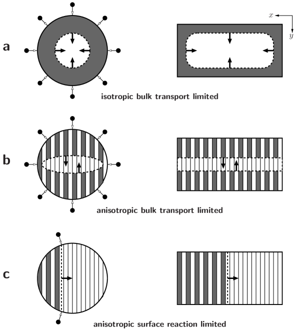
Figure 2: Transport models obtained in different limits of the characteristic timescales for bulk diffusion and surface reactions. Figures show $xy$ cross sections of spherical and plate-like single crystals during Li insertion, after phase nucleation has occurred. Lithiated portions of the crystal are shaded, and points outside particles represent flux of Li ions across the electrode/electrolyte interface (shown only for spherical particles). The FePO₄/LiFePO₄ phase boundary is denoted by the dashed line, and arrows indicate movement of the boundary as insertion proceeds. (a) Isotropic bulk transport limited. (b) Anisotropic bulk transport limited. (c) Anisotropic surface reaction limited.

In this initial effort, we neglect the possibility of charge separation and assume that electrons are freely available in the material to compensate the charge of Li⁺, although the presence of multiple diffusing and migrating species (interacting through an electrostatic potential) can be modeled as an extension of the general framework we present. We also avoid an explicit treatment of stress around the FePO₄/LiFePO₄ interface; instead, we note that a term in the phase field formulation may serve as an approximation of the energy due to the lattice mismatch.

II General Model

II.1 Phase field formulation

We follow the conventional Cahn-Hilliard formulation Cahn and Hilliard (1958) that has been previously applied as a phase field model for bulk transport in LiFePO₄ Han et al. (2004). The total free energy of the system is expressed as a functional of the local Li concentration

$$F=\int\left[\bar{f}(c)+(K/2)|\nabla c|^{2}\right]d\mathbf{r},$$ (6)

where $c$ is the dimensionless, normalized Li concentration ($0<c<1$), $\bar{f}(c)$ is the homogeneous free energy density, and $K$ is the gradient energy coefficient that represents the energy penalty for maintaining concentration gradients in the system. The lattice mismatch at the FePO₄/LiFePO₄ phase boundary coincides with the concentration gradient, so the gradient penalty in (6) can be regarded as approximating related contributions the free energy. Phase-field models have also been developed, which include the long-range elastic contributions to the free energy Khachaturyan (1983); Larche and Cahn (1985), but here we restrict ourselves to the simpler formulation above, to allow us to focus on other effects, namely anisotropic transport and surface reactions. In this spirit, we also ignore any surface contributions to the free energy, such as the tension of the electrode/electrolyte interface.

The homogeneous, bulk free energy density takes the form of a regular solution model

$$\bar{f}(c)=ac(1-c)+\rho kT\left[c\ln c+(1-c)\ln(1-c)\right],$$ (7)

where $a$ is the average energy density (in a mean field sense) of the interaction between Li ions, $\rho$ is the number of intercalation sites per unit volume, $k$ is Boltzmann’s constant, and $T$ is the temperature. The first term in (7), the enthalpic contribution to the free energy, promotes separation of the system to $c=0$ or $c=1$, while the second term, the entropic contribution, favors mixing of the system. Therefore, the strength of the phase separation is characterized by the dimensionless ratio $\rho kT/a$. The chemical potential of Li in the FePO₄ host is calculated as the variational derivative

$$\mu =\frac{\delta F}{\delta c},$$ (8)

$$=\bar{\mu}-K\nabla^{2}c,$$ (9)

where we define $\bar{\mu}$ as the homogeneous chemical potential

$$\bar{\mu} =\frac{\partial\bar{f}}{\partial c},$$ (10)

$$=a(1-2c)+\rho kT\ln\left(\frac{c}{1-c}\right).$$ (11)

While in general, the two phase compositions in equilibrium across the miscibility gap are determined by the common tangent construction, in the symmetric free energy $\bar{f}$ of (7) these compositions correspond to $\bar{\mu}=0$. These roots cannot be found analytically from (11), but asymptotic approximations in the small parameter $\rho kT/a$ can be obtained; two term expansions are

$$c_{-} \sim e^{-\frac{a}{\rho kT}}\left(1+\frac{a}{\rho kT}e^{-\frac{a}{\rho kT}}\right),$$ (12)

$$c_{+} \sim 1-c_{-},$$ (13)

where $c_{-}$ is the root near $c=0$ and $c_{+}$ is the root near $c=1$. As may be expected, $c_{\pm}$ approach the concentration extremes exponentially in $a/(\rho kT)$. While nucleation may be required to form a second phase for compositions in the miscibility gap, spontaneous phase separation occurs when the composition is within the spinodals. The spinodals correspond to the zeros of the curvature of the free energy and can be determined from (7) as

$$c_{\text{sp}}=\frac{1\pm\sqrt{1-2\rho kT/a}}{2}.$$ (14)

We observe that $a>2\rho kT$ is required for distinct, physically meaningful spinodal compositions.

II.2 Anisotropic bulk transport

As described above, Li migration in the bulk crystal is confined to 1D channels in the (010) direction, labeled as $y$ in Fig. 2. Some diffusion in other directions may occur due to defects in the crystal lattice or cracks caused by the FePO₄/LiFePO₄ lattice mismatch, as have been observed experimentally Chen et al. (2006); Laffont et al. (2006). Experiments Chen et al. (2006); Laffont et al. (2006) have found that layers of stacked 1D channels in the $z$ direction are progressively filled or emptied as the phase boundary moves across the layers in the $x$ direction, indicating that transport in the $z$ direction is faster than transport in the $x$ direction. The anisotropic Li flux can be written as

$$\mathbf{j}=-c\mathbf{B}\nabla\mu,$$ (15)

where

$$\mathbf{B}=\begin{pmatrix}b_{11}&0&0\\ 0&b_{22}&0\\ 0&0&b_{33}\end{pmatrix}$$ (16)

is the mobility tensor for an orthorhombic crystal, and the indices 1, 2, 3 correspond to the $x$, $y$, $z$ directions, respectively. The diffusivity tensor is determined from the mobility by the Einstein relation $\mathbf{D}=kT\mathbf{B}$. Based on the discussion above, we expect that $b_{11}\ll b_{33}\ll b_{22}$. We also note that $\mathbf{D}$ can, in general, be position or concentration dependent. In fact, for some other intercalation materials that do not phase separate, first principles calculations have shown that the diffusivity is a highly nonlinear function of the Li concentration, varying by several orders of magnitude over the composition range der Ven and Ceder (2000).

With the ionic fluxes thus defined, the dynamics of the concentration profile is governed by the conservation law

$$\rho\frac{\partial c}{\partial t}+\nabla\cdot\mathbf{j}=0,$$ (17)

where the factor of $\rho$ is needed for dimensional consistency.

II.3 Surface reactions

We assume that Arrhenius kinetics govern the insertion and extraction rates of Li across the electrode/electrolyte interface. The activation energies for these interfacial reactions are defined as the change in the chemical potential of Li across the interface. We further assume that the chemical potential of Li in the FePO₄ host, $\mu$ given by (9), is valid everywhere on the electrode surface where Li transfer occurs, with the appropriate modification for the Laplacian term. By also using the bulk chemical potential for ions at the crystal surface, we are neglecting the possibility of any variation in the chemical potential at the electrode/electrolyte interface, e.g. due to surface orientation or surface curvature, as noted above Wang et al. (2007).

With these assumptions, the local Li insertion rate is

$$R_{\text{ins}}=k_{\text{ins}}c_{e}e^{(\mu_{e}-\mu)/(\rho kT)},$$ (18)

where $k_{\text{ins}}$ is the insertion rate coefficient, and $c_{e}$ and $\mu_{e}$ are the concentration and chemical potential of Li in the electrolyte, respectively. Note that since $c_{e}$ is expressed as a dimensionless filling fraction, $R_{\text{ins}}$ and $k_{\text{ins}}$ have dimensions of inverse time.

In a more complete battery model, $c_{e}$ and $\mu_{e}$ would be determined by solving the appropriate transport equations for Li in the electrolyte. However, as we focus here on Li transport in the electrode, we ignore variations in the electrolyte and take $c_{e}$ and $\mu_{e}$ as constants. Our formulation therefore describes potentiostatic, or constant chemical equilibrium, conditions in the electrolyte, with the interfacial transfer of Li as the rate limiting process. Absorbing $c_{e}$ into $k_{\text{ins}}$ gives

$$R_{\text{ins}} =k_{\text{ins}}e^{\alpha(\mu_{e}-\mu)},$$ (19)

$$=\bar{R}_{\text{ins}}e^{\alpha K\nabla^{2}c},$$ (20)

where $\alpha=1/(\rho kT)$, and $\bar{R}_{\text{ins}}$ is the homogeneous insertion rate

$$\bar{R}_{\text{ins}}=k_{\text{ins}}\left(\frac{1-c}{c}\right)e^{\alpha[\mu_{e}-a(1-2c)]}.$$ (21)

Similarly, the extraction rate is

$$R_{\text{ext}} =k_{\text{ext}}ce^{\alpha(\mu-\mu_{e})},$$ (22)

$$=\bar{R}_{\text{ext}}e^{-\alpha K\nabla^{2}c},$$ (23)

where $\bar{R}_{\text{ext}}$ is the homogeneous extraction rate

$$\bar{R}_{\text{ext}}=k_{\text{ext}}\left(\frac{c^{2}}{1-c}\right)e^{\alpha[a(1-2c)-\mu_{e}]}.$$ (24)

In contrast to $R_{\text{ins}}$, the proportionality of $R_{\text{ext}}$ on $c$ cannot be neglected and breaks the symmetry about $c=1/2$. The net rate of Li insertion is therefore

$$R =R_{\text{ins}}-R_{\text{ext}},$$ (25)

$$=\bar{R}_{\text{ins}}e^{\alpha K\nabla^{2}c}-\bar{R}_{\text{ext}}e^{-\alpha K\nabla^{2}c},$$ (26)

$$\begin{split}&=k_{\text{ins}}\left(\frac{1-c}{c}\right)e^{\alpha[\mu_{e}-a(1-2c)+K\nabla^{2}c]}\\ &\quad-k_{\text{ext}}\left(\frac{c^{2}}{1-c}\right)e^{\alpha[a(1-2c)-\mu_{e}-K\nabla^{2}c]}.\end{split}$$ (27)

The boundary conditions for (17) on the crystal surface express mass conservation at the electrode/electrolyte interface,

$$\mathbf{n}\cdot\mathbf{j}=-\rho_{s}R,$$ (28)

where $\mathbf{n}$ is the unit normal vector directed out of the crystal, and $\rho_{s}$ is the number of intercalation sites per unit area, which depends on the orientation of the surface. Consistent with our neglect of surface excess chemical potential, we neglect the possibility of a surface flux density $\mathbf{j}_{s}$, whose surface divergence $\nabla_{s}\cdot\mathbf{j}_{s}$ would appear as an extra term on the right hand side of (28).

III Surface-reaction-limited phase transformation

III.1 Depth-integrated dynamics

We now develop a special limit of the general model that describes SRL phase-transformation in LiFePO₄. We assume that fast diffusion in the $y$ oriented 1D channels rapidly equilibrates the bulk Li concentration to the surface concentration. A depth-averaged concentration $\bar{c}$ on the $xz$ surface can therefore be defined as

$$\bar{c}=\frac{1}{L_{y}(x,z)}\int c(x,y,z,t)\,dy,$$ (29)

where $L_{y}(x,z)$ is the depth of the crystal in the $y$ direction, from surface to surface.

By depth-averaging the bulk transport equation (17), using the boundary condition (28), we find that the dynamics of $\bar{c}$ are governed solely by the surface reaction rate $R$, acting as a source term on the $xz$ surface,

$$\left(\frac{\rho L_{y}(x,z)}{2\rho_{s}(x,z)}\right)\frac{\partial\bar{c}}{\partial t}=R(\bar{c},\nabla^{2}\bar{c}),$$ (30)

where $\rho_{s}(x,z)$ is the number of atoms per unit area, dependent on the local orientation of the crystal surface. As noted above, a surface diffusion term could also be explicitly added to (30), but we shall see that the reaction rate $R$ already produces weak $xz$ diffusion due the gradient penalty $K$, which suffices to propagate the phase boundary along the surface.

Equation (30) describes a fundamentally different type of phase transformation dynamics. From a mathematical point of view, the striking feature is that the Laplacian term $\nabla^{2}\bar{c}$ appears in a nonlinear source term, as opposed to the additive quasilinear term in classical reaction-diffusion equations. We are not aware of any prior study of this type of equation, so it begs mathematical analysis to characterize its solutions.

Here, we begin this task by making some simplifying assumptions, which allow us to highlight new nonlinear wave phenomena described by (30). As noted above, experiments indicate that layers of 1D channels along the $yz$ plane are progressively filled or emptied as Li transfer proceeds, so it is natural to neglect concentration variations in the $z$ direction as a first approximation, for a planar phase boundary spanning the crystal. We also neglect depth variations, $L_{y}=$ constant, and assume constant surface orientation, $\rho_{s}=$ constant, which corresponds to the common case of a plate-like crystal.

III.2 Dimensionless formulation

A dimensionless form of the model, suitable for mathematical analysis, is found by scaling each variable to its natural units. The Li concentration is already expressed as a dimensionless filling fraction per channel $\bar{c}$, which will depend on the dimensionless position $\tilde{x}=x/L$ and time $\tilde{t}=t/\tau$. Position is scaled to a length $L$, which characterizes the size of the crystal surface along which the SRL phase transformation propagates. The natural time scale from (30) is

$$\tau=\frac{\rho L_{y}}{2\rho_{s}k_{\text{ins}}},$$ (31)

which is the time required for the insertion reaction to fill a single fast-diffusion channel in the crystal (from both sides). Note that this time scale is proportional to the depth of the crystal, $L_{y}$.

There are four dimensionless groups which govern the solution. The first is the ratio of reaction-rate constants

$$\kappa=\frac{k_{\text{ext}}}{k_{\text{ins}}},$$ (32)

which measures asymmetry in the extraction and insertion reaction kinetics. By scaling energy density to the thermal energy density $\rho kT$, we arrive at three more dimensionless parameters:

$$\tilde{a}=\frac{a}{\rho kT},\quad\tilde{\mu}_{e}=\frac{\mu_{e}}{\rho kT},$$ (33)

and

$$\tilde{\lambda}=\sqrt{\frac{K}{\rho kTL^{2}}}=\frac{\lambda}{L}.$$ (34)

The latter formula makes it clear that the natural length scale for the phase boundary thickness, set by the gradient penalty in the free energy, is $\lambda=\sqrt{K/(\rho kT)}$. Since $\lambda$ is an atomic length scale (1 Å– 10 nm) much smaller than the crystal size (10 nm – 10 $\mu$m), the parameter $\tilde{\lambda}$ is typically small and lies in the range $10^{-5}<\tilde{\lambda}<1$.

With these scalings, the SRL phase-transformation equation (30) takes the dimensionless form

$$\begin{split}\frac{\partial\bar{c}}{\partial\tilde{t}}&=\left(\frac{1-\bar{c}}{\bar{c}}\right)e^{\tilde{\mu}_{e}-\tilde{a}(1-2\bar{c})+\tilde{\lambda}^{2}\frac{\partial^{2}\bar{c}}{\partial\tilde{x}^{2}}}\\ &\quad-\kappa\left(\frac{\bar{c}^{2}}{1-\bar{c}}\right)e^{\tilde{a}(1-2\bar{c})-\tilde{\mu}_{e}-\tilde{\lambda}^{2}\frac{\partial^{2}\bar{c}}{\partial\tilde{x}^{2}}},\end{split}$$ (35)

We will study solutions to this new nonlinear partial differential equation in the following sections, but we already can gain some insight by considering the limit of a sharp phase boundary, $\tilde{\lambda}\ll 1$, as discussed above. Expanding (35) for small $\tilde{\lambda}$, we obtain a reaction-diffusion equation at leading order,

$$\frac{\partial\bar{c}}{\partial\tilde{t}}=\tilde{\lambda}^{2}(\tilde{R}_{\text{ins}}+\tilde{R}_{\text{ext}})\frac{\partial^{2}\bar{c}}{\partial\tilde{x}^{2}}+(\tilde{R}_{\text{ins}}-\tilde{R}_{\text{ext}}),$$ (36)

where $\tilde{R}_{\text{ins}}$ and $\tilde{R}_{\text{ext}}$ are the dimensionless homogeneous reaction rates

$$\tilde{R}_{\text{ins}} =\left(\frac{1-\bar{c}}{\bar{c}}\right)e^{\tilde{\mu}_{e}-\tilde{a}(1-2\bar{c})}$$ (37)

$$\tilde{R}_{\text{ext}} =\kappa\left(\frac{\bar{c}^{2}}{1-\bar{c}}\right)e^{\tilde{a}(1-2\bar{c})-\tilde{\mu}_{e}}.$$ (38)

Thus, we see that (35) has a direct analog to a reaction-diffusion equation with a weak, concentration dependent diffusivity and nonlinear source term, in the appropriate physical limit of an atomically sharp phase boundary. The detailed structure and dynamics of the phase boundary, however, must be obtained by solving the full equation (35). Representative plots of the homogeneous net insertion rate $\tilde{R}_{\text{ins}}-\tilde{R}_{\text{ext}}$ are shown in Fig. 3.

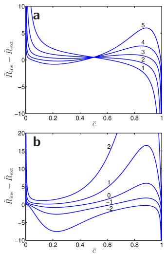
Figure 3: Dimensionless homogeneous net insertion rate. (a) $\tilde{\mu}_{e}=0$, $\kappa=1$, $\tilde{a}=1,\ldots,5$ as labeled in figure. (b) $\tilde{a}=5$, $\kappa=1$, $\tilde{\mu}_{e}=-2,\ldots,2$ as labeled in figure.

III.3 Traveling waves

We seek traveling wave solutions of (35), which physically correspond to waves of phase transformation, propagating through the FePO₄ crystal with steadily translating concentration profile. Since $\bar{c}$ is a depth averaged concentration, these composition waves extend through the bulk material to the surface, and they move parallel to the surface. Substituting the traveling-wave ansatz

$$\bar{c}(\tilde{x},\tilde{t})=g(\tilde{x}-\tilde{v}\tilde{t}),$$ (39)

into (35), where $\tilde{v}$ is the unknown constant velocity, and rewriting the resulting ordinary differential equation as a first-order system gives

$$g^{\prime} =h,$$ (40)

$$h^{\prime} =\frac{1}{\tilde{\lambda}^{2}}\ln\left[\frac{-\tilde{v}h+\sqrt{(\tilde{v}h)^{2}+4\kappa g}}{2\tilde{R}_{\text{ins}}(g)}\right],$$ (41)

where $g$ and $h$ are functions of $\zeta=\tilde{x}-\tilde{v}\tilde{t}$. The stationary points of the system are given by

$$h =0,$$ (42)

$$\tilde{a}(1-2g)+\ln\left(\frac{g^{3/2}}{1-g}\right)+\ln\Gamma =0,$$ (43)

where we define another dimensionless constant $\Gamma=e^{-\tilde{\mu}_{e}}\sqrt{\kappa}$.

The solutions of (43) correspond to the roots of the spatially homogeneous source $\tilde{R}_{\text{ins}}-\tilde{R}_{\text{ext}}$ and therefore determine the equilibrium phase compositions of the system. Explicit expressions for the solutions are not possible, though at least one solution must exist, since the left hand side changes sign over the interval $0<g<1$. However, phase separation into Li-poor and Li-rich phases requires three solutions $g_{1}<g_{2}<g_{3}$, where $g_{1}$ and $g_{3}$ are the equilibrium compositions bounding the moving wavefront, and $g_{2}$ is an unstable intermediate composition. We observe that the phase compositions are independent of the dimensionless gradient penalty $\tilde{\lambda}^{2}$. At the threshold where (43) transitions from one solution to three, the solutions and extrema of the equation coincide. The extrema occur at the compositions

$$g_{\pm}=\frac{(1+4\tilde{a})\pm\sqrt{16\tilde{a}^{2}-40\tilde{a}+1}}{8\tilde{a}},$$ (44)

and as two distinct extrema are needed for three solutions of (43), phase separation requires $\tilde{a}>5/4+\sqrt{3/2}\approx 2.47$. If the minimum $\tilde{a}$ is exceeded, (43) can be used to compute the rate coefficients and electrolyte chemical potential, expressed through the combination $\Gamma$, that will make either $g_{\pm}$ the critical composition at threshold. For strongly phase separating systems, such as LiFePO₄, we find asymptotic approximations of the solutions of (43) in the small parameter $1/\tilde{a}$. Two term expansions for each root are

$$g_{1} \sim e^{-\tfrac{2\tilde{a}}{3}}\left(\frac{1}{\Gamma^{2/3}}+\frac{4\tilde{a}e^{-\tfrac{2\tilde{a}}{3}}}{3\Gamma^{4/3}}\right),$$ (45)

$$g_{2} \sim\frac{1}{2}-\frac{1}{2}\ln\left(\frac{\sqrt{2}}{\Gamma}\right)\left[\frac{1}{\tilde{a}}-\frac{5}{2\tilde{a}^{2}}\right],$$ (46)

$$g_{3} \sim 1-e^{-\tilde{a}}\left(\Gamma+2\tilde{a}\Gamma^{2}e^{-\tilde{a}}\right).$$ (47)

The existence of traveling waves and the selection of the wave velocity in a phase separated system can be understood by a linear stability analysis of (40)–(41) about the three stationary points $(g_{i},0)$ for $i=1,2,3$. We find that $(g_{1},0)$ and $(g_{3},0)$ are saddle points for all velocities, and $(g_{2},0)$ is either a stable node or stable spiral, depending on the velocity. Monotonic wavefronts between the equilibrium Li-poor and Li-rich phases correspond to trajectories in the $(g,h)$ phase space that connect $(g_{1},0)$ and $(g_{3},0)$, bypassing $(g_{2},0)$. Following the continuity arguments presented in Murray (2002), there is a unique velocity $v$ such that the orientation of the eigenvectors at $(g_{1},0)$ and $(g_{3},0)$ allow a single trajectory joining these points. Thus, for a given set of parameters, all fully developed waves in a system propagate at the same velocity.

A rigorous mathematical analysis of the traveling wave solutions of (30), including their formal existence, stability, and velocity is beyond the scope of this work. Although analytical methods for studying traveling waves in parabolic systems are available Volpert et al. (1994), they are usually developed for systems where there is a diffusion term plus a source independent of derivatives of the solution, as in (36). To the best of our knowledge, (30) represents a different type of equation admitting traveling wave solutions, where the curvature dependence of the source precludes the need for an explicit diffusion term.

The nanoscale dimensions of the physical domain also complicate the analysis of (30). In other reaction diffusion equations, such as the Fisher equation, the wave velocity is determined by assuming an exponential decay of the leading edge of the wavefront as $\tilde{x}\rightarrow\infty$ Murray (2002). A finite cutoff in the leading edge is known to significantly alter the velocity Brunet and Derrida (1997). Such cutoffs are present in nanoparticles of LiFePO₄, as the $xz$ surface is bounded on the scale of the wave width. Moreover, the nanometer wave width describes the Li concentration across only a few atomic layers of the crystal, with each 1D channel in the layer holding a single file of Li atoms. Therefore, $\bar{c}$ may be discontinuous for small particles.

III.4 Wave propagation and nucleation

We investigate the traveling wave solutions of the SRL phase transformation model by numerically solving (35) with an explicit finite difference method, second order in space and time. Representative phase transformation waves during Li insertion and extraction are shown in Fig. 4. For these simulations, $\tilde{a}=5$ and $\tilde{\lambda}=1$, similar to the values given in Han et al. (2004). The choice of $\tilde{\lambda}$ corresponds to the dimensional lengthscales $\lambda=L=10$ nm. Although there is no available experimental or simulational data on the rate coefficients $k_{\text{ins}}$ and $k_{\text{ext}}$, we expect that the insertion and extraction reactions occur on the same timescale and therefore assume $\kappa=1$. Insertion or extraction is forced by raising or lowering the electrolyte chemical potential $\tilde{\mu}_{e}$ to promote transfer in one direction and inhibit transfer in the other; $\tilde{\mu}_{e}=0.5$ for the insertion process in Fig. 4a, and $\tilde{\mu}_{e}=-1$ for the extraction process in Fig. 4b. The initial conditions for the insertion and extraction waves, denoted by dashed lines in the plots, are Gaussian fluctuations of the composition representing nucleations of the lithiated and unlithiated phases, respectively. For the insertion in Fig. 4a, $\bar{c}(\tilde{x},0)=0.1+0.8\exp(-\tilde{x}^{2})$, and for the extraction in Fig. 4b, $\bar{c}(\tilde{x},0)=0.9-0.8\exp(-\tilde{x}^{2})$.

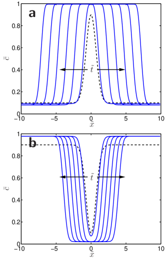
Figure 4: Numerically computed phase transformation waves during insertion and extraction. Dashed lines show initial conditions; solid lines show concentration profiles at uniformly spaced times, with arrows indicating direction of wave propagation. For both insertion and extraction: $\tilde{a}=5$, $\kappa=1$, $\tilde{\lambda}=1$. (a) Insertion wave with $\tilde{\mu}_{e}=0.5$, $\bar{c}(\tilde{x},0)=0.1+0.8\exp(-\tilde{x}^{2})$. (b) Extraction wave with $\tilde{\mu}_{e}=-1$, $\bar{c}(\tilde{x},0)=0.9-0.8\exp(-\tilde{x}^{2})$.

The initial composition fluctuation rapidly develops into two wavefronts bounded by the equilibrium Li-poor and Li-rich phases $g_{1}$ and $g_{3}$, respectively. The development of a fully formed wavefront involves both insertion and extraction. During the insertion process in Fig. 4a, the maximum concentration of the initial fluctuation grows to $g_{3}$, while the low concentration baseline decays to $g_{1}$. Conversely, for the extraction process in Fig. 4b, the minimum concentration decays to $g_{1}$, and the high concentration baseline grows to $g_{3}$. Once fully developed wavefronts form, they propagate to the right and left with a constant velocity. We have verified that the velocity of a fully developed wavefront is constant for all times in the numerical simulations, as expected from the phase plane analysis described earlier.

The dimensionless width $\tilde{w}$ and velocity $\tilde{v}$ of a fully developed wavefront are determined by the parameters of the system. The main parameter controlling the width of the wave is $\tilde{\lambda}$, since it contains the gradient energy coefficient $K$. As $\tilde{\lambda}$ is decreased, the energetic penalty for forming gradients in the concentration is lowered, resulting in sharper wavefronts spanning the equilibrium phase compositions. Additionally, we find that sharper wavefronts move at a slower velocity. The numerically computed dependence of the width and velocity on $\tilde{\lambda}$ is shown in Fig. 5. It is apparent that both $\tilde{w}$ and $\tilde{v}$ scale linearly with $\tilde{\lambda}$ in the range of physical relevance. In fact, this linear scaling can be determined analytically by a dimensional analysis of the system in the sharp interface limit $\tilde{\lambda}\ll 1$, as performed in the following section.

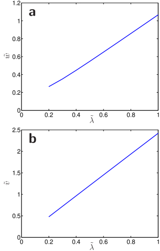
Figure 5: Scaling of computed wave (a) width and (b) velocity with $\tilde{\lambda}$. Parameters: $\tilde{a}=5$, $\kappa=1$, $\tilde{\mu}_{e}=0.5$, $\bar{c}(\tilde{x},0)=0.1+0.8\exp(-\tilde{x}^{2})$.

The electrolyte chemical potential $\tilde{\mu}_{e}$ is an experimentally accessible independent parameter, as it corresponds to the applied potential of the system, forcing Li insertion or extraction to occur. Thus, it is important to consider the dependence of the wave width and velocity on this parameter, as a systematic study of this dependence may eventually lead to an experimentally feasible method of testing the SRL model. Fig. 6 shows the numerically determined dependence of $\tilde{w}$ and $\tilde{v}$ on $\tilde{\mu}_{e}$. As shown in Fig. 6a, the wave width exhibits a weak, nonlinear dependence on $\tilde{\mu}_{e}$, embodied in the scaling function $F_{w}$ that arises in the dimensional analysis described in the following section. The velocity dependence in Fig. 6b shows how the system transitions from extraction waves to insertion waves as $\tilde{\mu}_{e}$ increases from negative to positive. Large negative values of $\tilde{\mu}_{e}$ strongly force Li removal, resulting in extraction waves with large velocities. As $\tilde{\mu}_{e}$ increases, the extraction wave velocity declines steeply, until zero velocity is obtained at $\tilde{\mu}_{e}\approx-0.5$. This point is the transition from extraction to insertion. Insertion waves with increasing velocities are produced as $\tilde{\mu}_{e}$ increases beyond the transition point. Analogously to the width, the velocity dependence is contained within a scaling function $F_{v}$ discussed in the following section. Note that the width and velocity profiles are not symmetric about the transition point, and the minimum width does not correspond to zero velocity. The asymmetry in the width and velocity result from the asymmetry in the homogeneous net reaction rate $\tilde{R}_{\text{ins}}-\tilde{R}_{\text{ext}}$. As described previously, $\tilde{R}_{\text{ins}}-\tilde{R}_{\text{ext}}$ must have three roots over the composition range $0<c<1$ in order for phase separation to occur. This requirement imposes a restricted range on $\tilde{\mu}_{e}$ for a given set of parameters. The extreme negative and positive values of $\tilde{\mu}_{e}$ in Fig. 6 are therefore fixed; there are no traveling wave solutions beyond them. The bounding values of $\tilde{\mu}_{e}$ can be determined analytically by solving (43) for the $\tilde{\mu}_{e}^{\mp}$ corresponding to the extrema $g_{\pm}$ given by (44), as these compositions define the limits of the phase separation range. We obtain

$$\tilde{\mu}_{e}^{\mp}=\tilde{a}(1-2g_{\pm})+\ln\left(\frac{g_{\pm}^{3/2}}{1-g_{\pm}}\right)+\ln\sqrt{\kappa},$$ (48)

where $\tilde{\mu}_{e}^{-}$ is the minimum allowable potential for extraction waves, and $\tilde{\mu}_{e}^{+}$ is the maximum allowable potential for insertion waves. The notational $\pm$ signs of $g_{\pm}$ and $\tilde{\mu}_{e}^{\mp}$ are reversed since $g_{-}$ is the minimum extremum at which there is almost only insertion, hence corresponding to the maximum allowable potential $\tilde{\mu}_{e}^{+}$, and conversely for $g_{+}$ and $\tilde{\mu}_{e}^{-}$. The limitations on $\tilde{\mu}_{e}$ are physically meaningful. In principle, transport can be driven by an arbitrarily positive or negative $\tilde{\mu}_{e}$. However, such a strong $\tilde{\mu}_{e}$ effectively increases the overall surface reaction rate $k$ and pushes the system out of the SRL transport regime $Da\ll 1$. Indeed, for sufficiently fast surface reactions, the system becomes a BTL process ($Da\gg 1$) with phase transformation governed by shrinking core type dynamics.

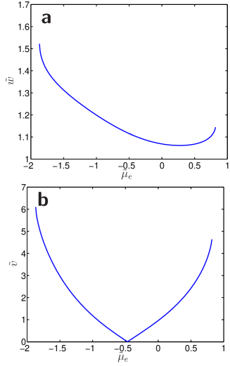
Figure 6: Dependence of computed wave (a) width and (b) velocity on $\tilde{\mu}_{e}$. Parameters: $\tilde{a}=5$, $\kappa=1$, $\tilde{\lambda}=1$, $\bar{c}(\tilde{x},0)=g_{1}(\tilde{\mu}_{e})+(1/2)(g_{3}(\tilde{\mu}_{e})-g_{1}(\tilde{\mu}_{e}))(\tanh(\tilde{x})+1)$.

Not all initial conditions give rise to traveling waves, as shown in Fig. 7. The key requirement for the formation of traveling waves is that the initial condition supports both addition and removal of Li in the domain, that is $R(x,0)$ must change sign. The simultaneous addition and removal of material sharpen the initial composition fluctuation to a phase separating wavefront. In the failed insertion event shown in Fig. 7a, only extraction occurs, and the initial composition perturbation decays to a uniform concentration of $g_{1}$. Similarly, Fig. 7b presents a failed extraction event where the initial composition depression fills up to a uniform concentration of $g_{3}$. Note that $R(x,0)$ depends on the Laplacian of the initial concentration profile $\bar{c}(x,0)$, and thus different initial conditions with equal composition ranges but varying spatial distributions will or will not produce traveling waves. This behavior has been numerically verified.

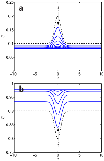
Figure 7: Numerically computed failed insertion and extraction events. Dashed lines show initial conditions; solid lines show concentration profiles at uniformly spaced times, with arrows indicating direction of profile movement. For both insertion and extraction: $\tilde{a}=5$, $\kappa=1$, $\tilde{\lambda}=1$. (a) Failed insertion event with $\tilde{\mu}_{e}=0.5$, $\bar{c}(\tilde{x},0)=0.1+0.1\exp(-\tilde{x}^{2})$. (b) Failed extraction event with $\tilde{\mu}_{e}=-1$, $\bar{c}(\tilde{x},0)=0.9-0.1\exp(-\tilde{x}^{2})$.

The dependence of the formation of traveling waves on the initial condition relates to the nucleation of the phase separation. During insertion, for example, the lithiated phase may first nucleate at some atomic scale inhomogeneity on the crystal surface where it is energetically favorable for Li atoms to collect. Our theory does not account for such features, and therefore it cannot model the initiation of the phase separation. Moreover, as the FePO₄/LiFePO₄ phase boundary width $\lambda$ is nearly at the atomic scale, applying a continuum equation for nucleation below this scale may not be physically relevant. We note, however, that continuum nucleation could be studied in other SRL systems with larger $\lambda$.

III.5 Scaling with material constants

A complete characterization of wave dynamics in the SRL regime is beyond the scope of this paper, but we conclude this section by summarizing some key features from the analysis above, with dimensions restored.

Wave nucleation. Starting from a pure phase and adjusting the external chemical potential in the electrolyte $\mu_{e}$, or the interaction strength $a$, the nucleation of a phase transition wave occurs whenever a random concentration fluctuation produces a region of sufficiently high, stable concentration of the opposite phase. The gradient penalty then sharpens the wave, and it propagates by the addition or removal of ions at the wavefront, due it its elevated chemical potential compared to both pure phases.

Wave width. By dimensional analysis, the width $w$ of the traveling wave profile is given by

$$w=LF_{w}\left(\frac{\lambda}{L},\frac{a}{\rho kT},\frac{\mu_{e}}{\rho kT},\frac{k_{\text{ext}}}{k_{\text{ins}}}\right)$$ (49)

where $F_{w}(\tilde{\lambda},\tilde{a},\tilde{\mu}_{e},\kappa)$ is a scaling function. Since the width $w$ should not depend on the size of the crystal $L$ in the limit of a sharp phase boundary, we have $\tilde{w}=F_{w}\sim\tilde{\lambda}f_{w}$ or $w\propto\lambda$ for $\tilde{\lambda}\ll 1$, consistent with the numerical solutions above in Fig. 5a. With units restored, we see that the width is set by the phase-boundary thickness

$$w\sim\sqrt{\frac{K}{\rho kT}}f_{w}\left(\frac{a}{\rho kT},\frac{\mu_{e}}{\rho kT},\frac{k_{\text{ext}}}{k_{\text{ins}}}\right)$$ (50)

as expected, although it may also depend weakly on $\tilde{a}$, $\tilde{\mu}_{e}$, and $\kappa$. A slice of the $\tilde{\mu}_{e}$ dependence is shown in Fig. 6a.

Wave speed. The speed of the traveling wave has a similar form,

$$v=\frac{L}{\tau}F_{v}\left(\frac{\lambda}{L},\frac{a}{\rho kT},\frac{\mu_{e}}{\rho kT},\frac{k_{\text{ext}}}{k_{\text{ins}}}\right)$$ (51)

where $F_{v}(\tilde{\lambda},\tilde{a},\tilde{\mu}_{e},\kappa)$ is another scaling function. Once again, the limit of a sharp phase boundary requires, $\tilde{v}=F_{v}\sim\tilde{\lambda}f_{v}$ or $v\propto\lambda/\tau$ for $\tilde{\lambda}\ll 1$, consistent with the numerical solutions in Fig. 5b.

Recalling the time unit, we obtain a general expression for the wave speed in the limit of a sharp phase boundary,

$$v\sim\sqrt{\frac{K}{\rho kT}}\frac{2\rho_{s}k_{\text{ins}}}{\rho L_{y}}f_{v}\left(\frac{a}{\rho kT},\frac{\mu_{e}}{\rho kT},\frac{k_{\text{ext}}}{k_{\text{ins}}}\right).$$ (52)

Note that the wave speed decreases with increasing crystal thickness, $v\propto 1/L_{y}$ since it takes longer for reactions to fill each bulk channel, as the SRL phase transformation proceeds sweeps across the crystal. The speed is also proportional to the gradient penalty coefficient $K$ and the insertion rate constant $k_{\text{ins}}$. It also should decrease with the strength of the interaction between ions in the crystal $a$, which drives phase separation. The wave velocity can also be controlled externally by varying the chemical potential of ions in the electrolyte $\mu_{e}$, as shown in Fig. 6b.

IV Response to an applied voltage

IV.1 BTL versus SRL dynamics

Transport in electrode materials is often studied by measuring the current response of the material to an applied potential. In an isotropic BTL process, a potential step induces a current proportional to the diffusion limited flux of ions across the electrode/electrolyte interface. The response time of any linear or nonlinear diffusion limited process, such as assumed in the shrinking core model, is given by the characteristic time $t_{D}-L^{2}/D$. The flux for small times, and hence the current, can be found analytically from the similarity solution for diffusion in a semi-infinite domain. The resulting expression for the current is known as the Cottrell equation,

$$I_{\text{Cottrell}}=neA\rho\sqrt{\frac{D}{\pi t}},\quad t\ll t_{D},$$ (53)

where $n$ is the number of electrons transferred and $A$ is the electrode particle area. The Cottrell current response forms the basis of the Potentiostatic Intermittent Titration Technique (PITT) that is commonly used to measure the diffusivity of materials Wen et al. (1979). However, cathodes that operate in a SRL transport regime where bulk diffusion in a preferred direction is fast relative to ion transfer at the electrode/electrolyte interface cannot be assumed to follow Cottrell dynamics.

In our model for single crystal LiFePO₄, the chemical potential of the electrolyte $\mu_{e}$ serves as the applied potential to the system. For an appropriate $\mu_{e}$, sharply defined waves of Li propagate across the crystal surface as Li transfer occurs. A composition fluctuation initiates each wave, and all fully developed waves in the system travel with the same, constant velocity, in a flat plate-like particle. The total flux of ions across the two $xz$ surfaces of the crystal is determined by the integral of the net insertion rate, so the current response of a single crystal is given by

$$I=ne\iint\!\rho_{s}R\,dx\,dz,$$ (54)

Note that since the reaction rate $R$ is zero at the equilibrium phase compositions $g_{1}$ and $g_{3}$, only localized wavefronts spanning these compositions contribute to the current.

The scaling of the SRL response is radically different from that of the Cottrell BTL response. Ignoring geometrical effects and nucleation (discussed below), the basic scaling of the response time for a single crystal is given by

$$t_{v}=\frac{L}{v}=\frac{L\tau}{\lambda}=L\sqrt{\frac{\rho kT}{K}}\frac{\rho L_{y}}{2\rho_{s}k_{\text{ins}}}.$$ (55)

Note that the response time is proportional to two geometrical lengths, the depth of the channels $L_{y}$ and the length $L$ over which the waves are propagating. More importantly, the time is determined by the surface reaction rate $k_{\text{ins}}$ and not by the bulk diffusion coefficient $D$. The ratio of the time scales for BTL dynamics and SRL dynamics is an effective Péclet number,

$$Pe=\frac{t_{D}}{t_{v}}=\frac{vL}{D}=\sqrt{\frac{K}{\rho kT}}\frac{2\rho_{s}k_{\text{ins}}L}{\rho L_{y}D}$$ (56)

which measures the importance of wave propagation at the diffusive time scale. However, this is once again the Damkohler number, since the reaction time is set by wave propagation, $t_{R}=t_{v}$, in the SRL regime.

IV.2 Plate-like crystals

To develop a general picture of SRL phase transformation dynamics in a rechargeable battery cathode, we first consider the case of flat plate-like crystals of constant depth $L_{y}$ analyzed in the previous section. A fully developed wavefront moving with constant velocity supports a steady current, and there is a sudden loss in the current when two wavefronts merge and are replaced by an equilibrium composition. Fig. 8 shows this declining staircase form for the current in a system with two impinging waves. The spike in the current at the time of collision is due to the gradient penalty term in the reaction rate acting on the sharp composition profile of the merging waves. We note that the magnitude of the spike is large in this simulation since there are only two waves; in an actual system with many waves, the surge in current from any individual collision would be small relative to the total current being sustained.

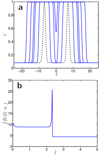
Figure 8: Numerically computed phase transformation dynamics and flux response of two impinging insertion waves. (a) Concentration profiles of impinging waves. Dashed line shows initial condition; solid lines show concentration profile at various times during impingement. (b) Flux response of impinging waves. Parameters: $\tilde{a}=5$, $\kappa=1$, $\tilde{\lambda}=1$, $\tilde{\mu}_{e}=0.5$, $\bar{c}(\tilde{x},0)=g_{1}+(g_{3}-g_{1})[\exp(-(\tilde{x}+7)^{2})+\exp(-(\tilde{x}-7)^{2})]$.

Thus, the current response of LiFePO₄ is governed by the overall rate of its transformation through concurrent nucleation and growth of waves. Phase nucleation likely occurs by both heterogeneous and homogeneous mechanisms. Recent first principles computations have found that the chemical potential of Li varies considerably over the surface of the equilibrium crystal shape Wang et al. (2007). Consequently, different crystal faces may be energetically favorable for heterogeneous phase nucleation during Li insertion and extraction.

An example of a single crystal undergoing heterogeneous and homogeneous nucleation and growth is illustrated in Fig. 9. Fig. 9a shows $xy$ cross sections of the crystal at a sequence of successive times $t_{1},\ldots,t_{6}$, and Fig. 9b presents the corresponding profile of the total current $I$. At time $t_{1}$, heterogeneous nucleation at the crystal edges has produced two fully developed wavefronts, each moving with constant velocity $v$ and sustaining a normalized current of unity. Therefore, the crystal supports the total current $I=2$ at this time. At some time between $t_{1}$ and $t_{2}$, heterogeneous nucleation occurs at the two rightmost surface defects of the crystal, indicated by notches. Once these nucleation events grow into fully developed waves, there are 6 propagating wavefronts carrying a total current of $I=6$. The rightmost waves merge at time $t_{3}$ such that 4 wavefronts are destroyed, and consequently, only two traveling wavefronts remain and the current drops to $I=2$. Homogeneous nucleation at some location in the untransformed fraction of the material occurs at time $t_{4}$, and the two additional wavefronts created increase the current to $I=4$. The rightmost waves combine at time $t_{5}$, and as most of the material is transformed and only two wavefronts remain, the current again drops to $I=2$. Finally, at time $t_{6}$, the material is fully transformed and can no longer sustain a current.

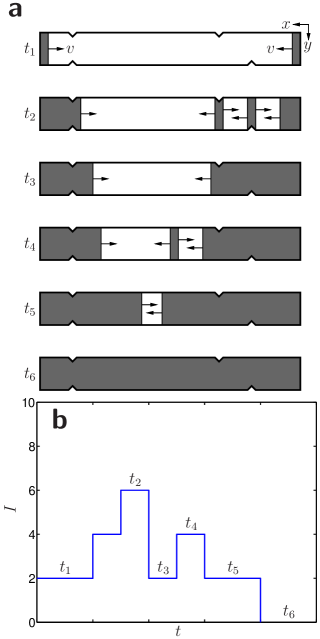
Figure 9: Schematic diagram of overall phase transformation and current response of a single plate-like crystal undergoing SRL transport. (a) Sequence of $xy$ cross sections of crystal at times $t_{1},\ldots,t_{6}$, illustrating phase transformation of material through concurrent nucleation and growth of traveling waves. Each fully developed wavefront moves with velocity $v$ and sustains a constant current of unity. (b) Declining staircase current response of crystal, with labeled times corresponding to illustrations in (a).

IV.3 Other crystal shapes

The wave dynamics can depend sensitively on the crystal shape in the SRL regime. This general fact can be easily seen from our analysis of a plate-like crystal: the wave velocity (52) depends on the local depth $L_{y}(x,z)$ of the fast diffusion channels in the bulk, as well as the local surface orientation, through the surface-site density $\rho_{s}(x,z)$. The analysis of SRL phase-transformation dynamics for arbitrary crystal shapes is a challenging problem, left for future work.

Here, we simply indicate how scalings by considering the limit of slowly varying depth, $L_{y}(x)$, and assuming the 1D wave dynamics for a flat surface are only slightly perturbed. The local wave velocity is then

$$v=\frac{dx_{w}}{dt}=\frac{D_{w}}{L_{y}(x_{w})}$$ (57)

where $D_{w}=2\rho_{s}(x_{w})k_{\text{ins}}\sqrt{K/(\rho^{3}kT)}\approx$ constant. This ordinary differential equation can be solved for the position of the wave $x_{w}(t)$ from a given wave nucleation event for any slowly varying shape $L_{y}(x_{w})$. For example, consider the case of a cylinder, $L_{y}(x)=\sqrt{R^{2}-x^{2}}$ (ignoring that the shape is not slowly varying at the ends). In that case, the equation can be solved analytically, e.g., for nucleation at one edge $x=-R$. For early times, the wave velocity decays from its initial value as $dx_{w}/dt\propto D_{w}^{2/3}t^{-1/3}$, due to the increasing depth of the bulk channels.

In spite of variable wave speed, however, the current remains constant during wave propagation in this approximation, as in the case of a flat plate, regardless of the crystal shape. The reason is that wave propagation at speed $v(x_{w})$ engulfs channels of length $L_{y}(x_{w})$, so the total current, proportional to $vL_{y}$, remains constant according to (57). The time for a wave to engulf the entire crystal thus scales with the total volume (in contrast to diffusive BTL dynamics, where the time scales like the cross-sectional area). Physically, ions are being inserted or extracted at roughly a constant rate, since the phase boundary is assumed to have a constant exposed length at the surface for 1D dynamics.

For spheres and other 3D shapes, the wavefront will not remain flat, and the full 2D depth-integrated dynamics will need to be solved with variable $L_{y}(x,z)$ and $\rho_{s}(x,z)$. However, the current may remains roughly constant during wave propagation, since the filling time for a channel is proportional to its length, at constant surface reaction rate. In that case, the results of the previous section for current versus time in flat plate-like single crystals may not be substantially modified with more complicated shapes, although statistical fluctuations due to random nucleation events will be different.

IV.4 Composite cathode response

It is important to note that Fig. 9 represents only one possible realization of the transformation and current response of the crystal. Heterogeneous nucleation may occur at different edges or surface defects at different times for different insertion and extraction cycles. Homogeneous nucleation would be spatially distributed in some random fashion. Therefore, to determine the overall current response of a composite cathode composed of many individual crystals, we must consider the statistical distributions of the nucleation events.

For homogeneous nucleation, we may assume that the nucleation rate is uniform across the crystal surface. Nucleation events in the untransformed material are independent, and the presence of a previously nucleated wave does not influence the likelihood of nucleation around that wave. With these assumptions, the nucleation events are distributed as a Poisson process in time, and we may invoke the Johnson-Mehl-Avrami equation for the overall transformation rate of the material Ballufi et al. (2005)

$$\xi=e^{-Gt^{n}},$$ (58)

where $\xi$ is the untransformed fraction of the material, $G$ is a factor dependent on the dimensionality of the process, and the integer $n>1$; for a 1D line nucleation process, $Gt^{n}\sim t^{2}$. The Johnson-Mehl-Avrami equation therefore specifies that the overall transformation rate of the material follows a sigmoidal shape. We thus expect that the current also follows this sigmoidal response for concurrent homogeneous nucleation and growth.

In the case of heterogeneous nucleation, we may assume that for many defects in many particles, the heterogeneous nucleation events are distributed as a Poisson process in space. Thus, the qualitative form of the average response is expected to follow the same sigmoidal shape as homogeneous nucleation, assuming all electrode particles are at the same potential (driving force), which may only be true under low rate conditions or for thin electrodes Delacourt et al. (2005); Gaberscek et al. (2007).

Thus, we have found that individual crystals have a declining staircase form for their current response to an applied electrolyte potential $\mu_{e}$ if a substantial number of nucleation events occur on the timescale of complete transformation. For many crystals, we may consider that the homogeneous and heterogeneous nucleation events are Poisson processes in time and space, respectively. The overall transformation and current response of the material is then given by the average of many distinct staircase responses, resulting in a characteristic sigmoidal curve

$$I\sim e^{-Gt^{n}},$$ (59)

that is strikingly different than the Cottrell response that is commonly assumed. Fig. 10 compares the sigmoidal and Cottrell responses. We conclude that PITT measurements in material undergoing SRL transport do not measure the diffusivity. Rather, these measurements provide some measure of the kinetic parameters in the surface reaction rates that are controlling the overall rate of the material transformation.

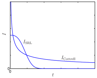
Figure 10: Schematic illustration of composite cathode responses for Cottrell (BTL) and SRL phase transformation mechanisms.

IV.5 Discussion

The model we propose is based on a few key experimental and theoretical findings. (1) Li migrates rapidly in the (010) direction ($y$ in Fig. 1) creating either filled or empty channels that completely penetrate the material. This makes it possible to coarse-grain to a two-dimensional model in which the surface concentration defines the concentration in a channel. (2) A linear interface exists on the particle surface between filled and unfilled sites, and growth of one phase at the expense of the other occurs by displacement of this interface. Such one-dimensional growth is supported by experimental observations Chen et al. (2006) and by a recent Johnson-Mehl Avrami analysis of the growth exponents Allen et al. (2007). Since one would expect two-dimensional growth on the surface for an isotropic material, the one-dimensional growth has to find its origin in the crystallography of the material. Undoubtedly, it is either the anisotropy of the interfacial strain energy - because of different coherence strains or elastic constants Maxisch and Ceder (2006), or the anisotropy of the interfacial energy which causes the system to prefer a single interface plane.

In our model, the transformation rate is controlled by transfer of the ions from the electrolyte to the (010) surface. Since during growth insertion only takes place at the interface, the energy of the Li ions at this interface is a key quantity in determining the effective transfer rate from the solution. Unlike in a core-shell model where the ability of the particle to take up current declines as (de)lithiation proceeds, in our model the transformation rate is nominally constant, until the particle is either fully transformed, new nucleation events occur, or two wave fronts impinge. Such transformation kinetics is fundamentally different from Cottrell-like behavior.

How this transformation kinetics manifests itself in the observable voltage-current response may depend very much on the structure of the macroscopic electrode in which the active LiFePO₄ particles are embedded. In addition to the active material, a typical electrode contains about 5–10 wt% polymeric binder and 5–15 wt% carbon black to enhance electronic conductivity through the electrode. Some porosity is also created in the electrode to allow the electrolyte to penetrate and transport the Li⁺ ions to and from the active material. If the conductive pathways for the Li⁺ ions and electrons are sufficient, all particles will be at the same potential and experience a similar driving force for transformation. Under these conditions, and assuming stochastic nucleation, we expect that the overall current response to a potential pulse is sigmoidal. Recent work indicates that such equipotential conditions across the electrode only apply at rather low charge and discharge rates, or for very thin electrodes Gaberscek et al. (2007). If such electrical resistance along the thickness of the electrode plays a role, the collective current response of the system could be viewed as of a sum of sigmoidals, each with a different driving force, but time-dependent screening effects would also need to be taken into account.

V Conclusion

We have proposed a general continuum theory for Li transport in single crystal LiFePO₄ based on a thermodynamically sound phase field formulation of the free energy. In various limits of the characteristic timescales for bulk and surface transport, this theory captures the shrinking core and other BTL models. In the limit where fast bulk diffusion in 1D equilibrates the bulk concentration to the surface concentration, our model gives a new type of equation describing SRL phase transition dynamics. We find that this model exhibits traveling wave solutions that qualitatively agree with the experimental observations. The main implication of our work for battery modeling is that the current response of SRL systems, such as LiFePO₄, are not governed by the classical, bulk diffusion limited Cottrell model that is commonly assumed. Our work also focuses attention to the importance of the Li⁺ and electron delivery to the proper surface of LiFePO₄ in order to achieve fast charge absorption. While much effort in the experimental literature has focused on electron delivery (e.g. by carbon coating or conductive Fe₂P contributions) Ravet et al. (2001); Herle et al. (2004), little emphasis seems to have been place on rapid transport of Li⁺ towards the surface where it can penetrate. Finally, we note that the SRL model developed here may be applicable in other materials where surface transfer effects are rate limiting, such as nanoporous materials.