Abstract

The Euler’s equations describe the motion of inviscid fluid. In the case of shallow water, when a perturbative asymtotic expansion of the Euler’s equations is taken (to a certain order of smallness of the scale parameters), relations to certain integrable equations emerge. Some recent results concerning the use of integrable equation in modeling the motion of shallow water waves are reviewed in this contribution.

Key Words: Euler’s equations, Integrability, Camassa-Holm equation, Degasperis-Procesi equation, Korteweg-de Vries equation.

1 Governing equations for the inviscid fluid motion

The motion of inviscid fluid with a constant density $\rho$ is described by the Euler’s equations:

$$\frac{\partial{\bf v}}{\partial t}+({\bf v}\cdot\nabla){\bf v} = -\frac{1}{\rho}\nabla P+{\bf g},$$ (1)

$$\nabla\cdot{\bf v} = 0,$$ (2)

where ${\bf v}(x,y,z,t)$ is the velocity of the fluid at the point $(x,y,z)$ at the time $t$, $P$ is the pressure in the fluid, ${\bf g}=(0,0,-g)$ is the constant Earth’s gravity acceleration.

Consider now a motion of a shallow water over a flat bottom, which is located at $z=0$. We assume that the motion is in the $x$-direction, and that the physical variables do not depend on $y$. Let $h$ be the mean level of the water and let $\eta(x,t)$ describes the shape of the water surface, i.e. the deviation from the average level. The pressure is

$$P=P_{A}+\rho g(h-z)+p(x,z,t),$$ (3)

where $P_{A}$ is the constant atmospheric pressure, and $p$ is a pressure variable, measuring the deviation from the hydrostatic pressure distribution. On the surface $z=h+\eta$, $P=P_{A}$ and therefore $p=\eta\rho g$. Taking ${\bf v}\equiv(u,0,w)$ we can write the kinematic condition on the surface as [e.g. see (Johnson 1997)]

$$w=\frac{\partial\eta}{\partial t}+u\frac{\partial\eta}{\partial x}\qquad\text{on}\qquad z=h+\eta.$$ (4)

Finally, there is no horizontal velocity at the bottom, thus

$$w=0\qquad\text{on}\qquad z=0.$$ (5)

The equations (1) – (5) give the system

$$u_{t}+uu_{x}+wu_{z}=-\frac{1}{\rho}p_{x},$$

$$w_{t}+uw_{x}+ww_{z}=-\frac{1}{\rho}p_{z},$$

$$u_{x}+w_{z}=0,$$

$$w=\eta_{t}+u\eta_{x},\quad p=\eta\rho g,\qquad\text{on}\qquad z=h+\eta,$$

$$w=0\qquad\text{on}\qquad z=0.$$

Let us introduce now dimensionless parameters $\varepsilon=a/h$ and $\delta=h/\lambda$, where $a$ is the typical amplitude of the wave and $\lambda$ is the typical wavelength of the wave. Now we can introduce dimensionless quantities, according to the magnitude of the physical quantities, see (Johnson 1997, 2002) for details:

$$x\rightarrow\lambda x,\qquad z\rightarrow zh,\qquad t\rightarrow\frac{\lambda}{\sqrt{gh}}t,\qquad\eta\rightarrow a\eta,\qquad$$

$$u\rightarrow\varepsilon\sqrt{gh}u,\qquad w\rightarrow\varepsilon\delta\sqrt{gh}w,\qquad p\rightarrow\varepsilon\rho gh.$$

This scaling is due to the observation that both $w$ and $p$ are proportional to $\varepsilon$ i.e. the wave amplitude, since at undisturbed surface ($\varepsilon=0$) both $w=0$ and $p=0$. The system (LABEL:S1) in the new, dimensionless variables is

$$u_{t}+\varepsilon(uu_{x}+wu_{z})=-p_{x},$$

$$\delta^{2}(w_{t}+\varepsilon(uw_{x}+ww_{z}))=-p_{z},$$

$$u_{x}+w_{z}=0,$$

$$w=\eta_{t}+\varepsilon u\eta_{x},\quad p=\eta,\qquad\text{on}\qquad z=1+\varepsilon\eta,$$

$$w=0\qquad\text{on}\qquad z=0.$$

For the right-running waves one can introduce the so-called far field quantities, see (Johnson 1997, 2002, 2003$a$)

$$\zeta=\sqrt{\varepsilon}(x-t),\qquad\tau=\varepsilon^{3/2}t,\qquad w=\sqrt{\varepsilon}W,$$ (8)

and the system (LABEL:S2) acquires the form

$$\varepsilon u_{\tau}-u_{\zeta}+\varepsilon(uu_{\zeta}+Wu_{z})=-p_{\zeta},$$ (9)

$$\varepsilon\delta^{2}(\varepsilon W_{\tau}-W_{\zeta}+\varepsilon(uW_{\zeta}+WW_{z}))=-p_{z},$$ (10)

$$u_{\zeta}+W_{z}=0,$$ (11)

$$W=\varepsilon\eta_{\tau}-\eta_{\zeta}+\varepsilon u\eta_{\zeta},\quad p=\eta,\qquad\text{on}\qquad z=1+\varepsilon\eta,$$ (12)

$$W=0\qquad\text{on}\qquad z=0.$$ (13)

2 Asymptotic expansion of the variables

Following the idea of Johnson (2002), we can express the variables $u$, $W$, $p$ as double-asymptotic expansion (in $\varepsilon$ and $\delta$) with terms, depending only on $\eta(x,t)$ and explicitly on $z$. As a result, a single nonlinear equation for $\eta$ will be obtained, and thus all variables will be expressed through the solution of this equation.

From (10) it is evident that $p_{z}=O(\varepsilon\delta^{2})$, and thus in the leading order $p$ does not depend on $z$, i.e.

$$p=\eta.$$ (14)

Substitution of (14) into (9) and (11) gives for the leading orders

$$u=\eta,\qquad W=-z\eta_{\zeta}.$$ (15)

Consider the next terms (first corrections) in the expansion of $u$ and $W$, denoted by $E(u)$, $E(W)$, which possibly contain terms of orders $\varepsilon$ and $\delta^{2}$. Writing $u=\eta+E(u)$, $W=-z\eta_{\zeta}+E(W)$, from (9) it follows

$$E_{\zeta}(u)=\varepsilon(\eta_{\tau}+\eta\eta_{\zeta}),$$ (16)

and from (11), (13) and (16),

$$E(W) = -\int E_{\zeta}(u){\text{d}}z=-\varepsilon z(\eta_{\tau}+\eta\eta_{\zeta}),$$

$$W = -z(\eta_{\zeta}+\varepsilon\eta_{\tau}+\varepsilon\eta\eta_{\zeta}).$$ (17)

Now the substitution of (17) into (12) gives the leading order equation for $\eta$:

$$\eta_{\tau}=-\frac{3}{2}\eta\eta_{\zeta}+O(\varepsilon,\delta^{2}).$$ (18)

From (18) and (16) we obtain $E(u)=-\varepsilon\eta^{2}/4$, i.e. no $\delta^{2}$ term is present and finally, using (17) and (18),

$$u=\eta-\frac{\varepsilon}{4}\eta^{2},\qquad W=-z\Big{(}\eta_{\zeta}-\frac{\varepsilon}{2}\eta\eta_{\zeta}\Big{)}.$$ (19)

Using (15) in (10) we have $p_{z}=-\varepsilon\delta^{2}z\eta_{\zeta\zeta}$. This can be integrated due to (12) and thus we obtain the next order approximation for $p$:

$$p=\eta-\varepsilon\delta^{2}\frac{1-z^{2}}{2}\eta_{\zeta\zeta}.$$ (20)

We accomplished the first step, i.e. starting from the leading order (14), (15), we obtained the first corrections (19), (20) and an equation for $\eta$, (18). The next step can be performed in a similar fashion and it gives

$$u = \eta-\frac{\varepsilon}{4}\eta^{2}+\frac{\varepsilon^{2}}{8}\eta^{3}+\varepsilon\delta^{2}\Big{(}\frac{1}{3}-\frac{z^{2}}{2}\Big{)}\eta_{\zeta\zeta},$$ (21)

$$W = -z\Big{(}\eta_{\zeta}-\frac{\varepsilon}{2}\eta\eta_{\zeta}+\frac{3\varepsilon^{2}}{8}\eta^{2}\eta_{\zeta}\Big{)}+\varepsilon\delta^{2}\Big{(}-\frac{z}{3}+\frac{z^{3}}{6}\Big{)}\eta_{\zeta\zeta\zeta},$$ (22)

$$p = \eta-\varepsilon\delta^{2}\frac{1-z^{2}}{2}\eta_{\zeta\zeta}+\varepsilon^{2}\delta^{2}(\eta\eta_{\zeta\zeta}+(1-z^{2})\eta^{2}_{\zeta}),$$ (23)

where $\eta(x,t)$ satisfies the equation

$$\eta_{\tau}=-\frac{3}{2}\eta\eta_{\zeta}+\frac{3}{8}\varepsilon\eta^{2}\eta_{\zeta}-\frac{1}{6}\delta^{2}\eta_{\zeta\zeta\zeta}+O(\varepsilon^{2},\delta^{4},\varepsilon\delta^{2}).$$ (24)

We observe, that at the end of each step the equation for $\eta(x,t)$ contains terms of smaller order than those, which appear in the expressions for $u$ and $W$. Since we need an equation, containing terms of order $O(\varepsilon^{2},\delta^{4},\varepsilon\delta^{2})$, we need to perform several intermediate sub-steps, (like (16), (17)) of the next step, which leads to the desired equation

$$\eta_{\tau}=-\frac{3}{2}\eta\eta_{\zeta}+\frac{3}{8}\varepsilon\eta^{2}\eta_{\zeta}-\frac{3}{16}\varepsilon^{2}\eta^{3}\eta_{\zeta}-\frac{1}{6}\delta^{2}\eta_{\zeta\zeta\zeta}\phantom{******}$$

$$-\frac{1}{24}\varepsilon\delta^{2}(23\eta_{\zeta}\eta_{\zeta\zeta}+10\eta\eta_{\zeta\zeta\zeta})+O(\varepsilon^{3},\delta^{6},\varepsilon^{2}\delta^{2},\varepsilon\delta^{4}).$$ (25)

Now, we can invert (21) by specifying $u$ at a specific depth, $z_{0}$

($0\leq z_{0}\leq 1$): defining $\hat{u}=u(\zeta,\tau,z_{0})$, we obtain

$$\eta=\hat{u}+\frac{\varepsilon}{4}\hat{u}^{2}-\varepsilon\delta^{2}\lambda\hat{u}_{\zeta\zeta}+O(\varepsilon^{3},\delta^{6},\varepsilon\delta^{4},\varepsilon^{2}\delta^{2}),$$ (26)

where

$$\lambda\equiv\frac{1}{3}-\frac{z_{0}^{2}}{2},\qquad-\frac{1}{6}\leq\lambda\leq\frac{1}{3}.$$ (27)

Note that in (26) there is no term of order $\varepsilon^{2}$. The substitution of (26) in (25) yields:

$$\hat{u}_{\tau}=-\frac{3}{2}\hat{u}\hat{u}_{\zeta}-\frac{1}{6}\delta^{2}\hat{u}_{\zeta\zeta\zeta}-\frac{1}{2}\varepsilon\delta^{2}\Big{[}\Big{(}\frac{29}{12}+6\lambda\Big{)}\hat{u}_{\zeta}\hat{u}_{\zeta\zeta}+\frac{5}{6}\hat{u}\hat{u}_{\zeta\zeta\zeta}\Big{]}\phantom{***}$$

$$+O(\varepsilon^{3},\delta^{6},\varepsilon^{2}\delta^{2},\varepsilon\delta^{4}).$$ (28)

Next, we go back to the original variables, introducing $T\equiv\sqrt{\varepsilon}t$, $X\equiv\sqrt{\varepsilon}x$, see (8), keeping only the scaling with $\varepsilon$ :

$$T=\frac{1}{\varepsilon}\tau,\qquad X=\frac{1}{\varepsilon}\tau+\zeta,$$ (29)

or $\partial_{\zeta}=\partial_{X}$, $\varepsilon\partial_{\tau}=\partial_{T}+\partial_{X}.$ Thus, (28) yields

$$\hat{u}_{T}=-\hat{u}_{X}-\frac{3}{2}\varepsilon\hat{u}\hat{u}_{X}-\frac{1}{6}\varepsilon\delta^{2}\hat{u}_{XXX}-\frac{1}{2}\varepsilon^{2}\delta^{2}\Big{[}\Big{(}\frac{29}{12}\!+\!6\lambda\Big{)}\hat{u}_{X}\hat{u}_{XX}+\frac{5}{6}\hat{u}\hat{u}_{XXX}\Big{]}$$

$$+O(\varepsilon^{4},\varepsilon\delta^{6},\varepsilon^{3}\delta^{2},\varepsilon^{2}\delta^{4}).\phantom{*}$$ (30)

Further, we add formally $(\varepsilon\delta^{2}\mu\hat{u}_{XXT}-\varepsilon\delta^{2}\mu\hat{u}_{XXT})/2$ to the left-hand side of (30), where $\mu$ is an arbitrary real parameter. In the first term we substitute $\hat{u}_{T}=-\hat{u}_{X}-\frac{3}{2}\varepsilon\hat{u}\hat{u}_{X}$, according to (30):

$$\Big{(}\hat{u}-\frac{1}{2}\varepsilon\delta^{2}\mu\hat{u}_{XX}\Big{)}_{T}=-\hat{u}_{X}-\frac{3}{2}\varepsilon\hat{u}\hat{u}_{X}+\varepsilon\delta^{2}(\frac{1}{2}\mu-\frac{1}{6})\hat{u}_{XXX}\phantom{********}$$

$$-\frac{1}{2}\varepsilon^{2}\delta^{2}\Big{[}\Big{(}\frac{29}{12}+6\lambda-\frac{9}{2}\mu\Big{)}\hat{u}_{X}\hat{u}_{XX}+\Big{(}\frac{5}{6}-\frac{3}{2}\mu\Big{)}\hat{u}\hat{u}_{XXX}\Big{]}$$

$$+O(\varepsilon^{4},\varepsilon\delta^{6},\varepsilon^{3}\delta^{2},\varepsilon^{2}\delta^{4}).$$ (31)

We observe that (30), (31) do not contain terms of orders $\varepsilon$ and $\varepsilon^{2}$. Thus, the set-up from (Johnson 2002) naturally leads to the conclusion, that equations, containing nonlinearities as those, appearing in the equations of Camassa $\&$ Holm (1993), Fokas $\&$ Fuchssteiner (1981) [called also CH from now on] and Degasperis $\&$ Procesi (1999), Degasperis et al. (2002) [DP for short], are generalizations of the Korteweg-de Vries equation, containing the next order term ($\varepsilon^{2}\delta^{2}$) in the expansion with respect to the small parameters $\varepsilon$, $\delta$.

3 Integrable nonlinear equations

In this section we start from a known integrable equation and we try to write it in a form, in which it matches (31) or (30). For another approach for matching between water waves equations and integrable equations see (Dullin et al. 2003, 2004). The CH and DP equations can be written as

$$(U-U_{XX})_{T}=\omega U_{X}-(b+1)UU_{X}+bU_{X}U_{XX}+UU_{XXX},$$ (32)

where $U=U(X,T)$, $\omega$ is an arbitrary constant, $b=2$ for CH and $b=3$ for DP. There is no other choice of the constant coefficients in front of the nonlinear terms, leading to integrable equations, see (Ivanov 2005$a$). Let us change the variables in (32) according to

$$X\rightarrow X-vT,\qquad T\rightarrow T,\qquad U\rightarrow U+C,$$ (33)

where $v$ and $C$ are arbitrary constants. Then (32) acquires the form

$$(U-U_{XX})_{T}=[\omega-(b+1)C+v]U_{X}+(C-v)U_{XXX}\phantom{******}$$

$$-(b+1)UU_{X}+bU_{X}U_{XX}+UU_{XXX}.$$ (34)

It is now clear that via the transforms (33) one can achieve arbitrary coefficients for the linear terms $U_{X}$ and $U_{XXX}$. Let us now consider the following scaling of the variables:

$$X\rightarrow\frac{1}{\alpha}X,\qquad T\rightarrow\beta T,\qquad U\rightarrow\gamma U.$$ (35)

Then (34) can be written as

$$(U-\alpha^{2}U_{XX})_{T}=\Gamma_{1}U_{X}+\Gamma_{2}U_{XXX}-\alpha\beta\gamma(b+1)UU_{X}\phantom{*****}$$

$$+\alpha^{3}\beta\gamma(bU_{X}U_{XX}+UU_{XXX}),$$ (36)

where $\Gamma_{1,2}$ are arbitrary constants. In order to match (36) to (31) up to the given order, we need to make the following identifications:

$$\alpha^{2}=\frac{1}{2}\varepsilon\delta^{2}\mu,\qquad\alpha\beta\gamma(b+1) = \frac{3}{2}\varepsilon,\qquad\alpha^{3}\beta\gamma=-\frac{1}{2}\Big{(}\frac{5}{6}-\frac{3}{2}\mu\Big{)}\varepsilon^{2}\delta^{2},$$

$$\frac{29}{12}+6\lambda-\frac{9}{2}\mu = b\Big{(}\frac{5}{6}-\frac{3}{2}\mu\Big{)}$$ (37)

which are compatible iff

$$\mu=\frac{5(b+1)}{9b},\qquad\lambda=\frac{30-9b}{72b}.$$ (38)

Thus, (38) and (27) show that (36) describes water waves at depth

$$z_{0}=\sqrt{\frac{11b-10}{12b}},$$ (39)

i.e. CH ($b=2$) corresponds to $z_{0}=\frac{1}{\sqrt{2}}\approx 0.71$ and DP ($b=3$) corresponds to $z_{0}=\sqrt{\frac{23}{36}}\approx 0.80$. The scaling coefficients from (37) are

$$\alpha=\sqrt{\frac{\mu}{2}}\varepsilon^{1/2}\delta,\qquad\beta\gamma=\frac{3}{\sqrt{2\mu}(b+1)}\varepsilon^{1/2}\delta^{-1},$$ (40)

and, apparently only the product $\beta\gamma$ is determined, i.e. there is additional freedom in the choice of $\beta$ and $\gamma$, one can take, for simplicity, just $\gamma=1$ and then, finally,

$$\alpha=\sqrt{\frac{\mu}{2}}\varepsilon^{1/2}\delta,\qquad\beta=\frac{3}{\sqrt{2\mu}(b+1)}\varepsilon^{1/2}\delta^{-1},\qquad\gamma=1.$$ (41)

Another equation, which passes the integrability check developed in (Mikhailov $\&$ Novikov 2002; Sanders $\&$ Jing Ping Wang 1998; Olver $\&$ Jing Ping Wang 2000) and is presumably integrable (although we do not have a proof of this fact – the test provides only a necessary condition for integrability) is

$$(U-U_{XX}+U_{XXXX})_{T}=\Gamma_{1}U_{X}-\Gamma_{2}U_{XXX}+\Gamma_{2}U_{XXXXX}\phantom{******}$$

$$-UU_{X}+U_{X}U_{XX}-U_{X}U_{XXXX},$$ (42)

where $\Gamma_{1,2}$ are arbitrary constants. This equation contains nonlinearities, similar to those, appearing in the nonintegrable equations studied by Holm $\&$ Hone (2003).

The scaling (35) gives

$$(U-\alpha^{2}U_{XX}+\alpha^{4}U_{4X})_{T} = \alpha\beta\Gamma_{1}U_{X}-\alpha^{3}\beta\Gamma_{2}U_{XXX}+\alpha^{5}\beta\Gamma_{2}U_{5X}$$

$$- \!\!\!\alpha\beta\gamma UU_{X}+\alpha^{3}\beta\gamma U_{X}U_{XX}-\alpha^{5}\beta\gamma U_{X}U_{4X},$$

The matching between (LABEL:eq41) and (31) leads to the following identifications:

$$\alpha^{2} = \frac{1}{2}\varepsilon\delta^{2}\mu,\qquad\alpha\beta\gamma=\frac{3}{2}\varepsilon,\qquad\alpha^{3}\beta\gamma=-\frac{1}{2}\Big{(}6\lambda-\frac{9}{2}\mu+\frac{29}{12}\mu\Big{)}\varepsilon^{2}\delta^{2},$$

$$\mu = \frac{5}{9}.$$ (44)

In a similar way, from (LABEL:eq41) we find (assuming again $\gamma=1$)

$$\lambda=-\frac{1}{8},\qquad z_{0}=\sqrt{\frac{11}{12}}\approx 0.96;$$ (45)

$$\alpha=\sqrt{\frac{\mu}{2}}\varepsilon^{1/2}\delta,\qquad\beta=\frac{3}{\sqrt{2\mu}}\varepsilon^{1/2}\delta^{-1},\qquad(\gamma=1).$$ (46)

The terms with fourth and fifth derivative in (LABEL:eq41) are of orders

$$\alpha^{4}=\frac{\mu^{2}}{4}\varepsilon^{2}\delta^{4},\qquad\alpha^{5}\beta=\frac{3\mu^{2}}{8}\varepsilon^{3}\delta^{4},\qquad\alpha^{5}\beta\gamma=\frac{3\mu^{2}}{8}\varepsilon^{3}\delta^{4},$$ (47)

and, therefore are small, in comparison to the other terms.

Another set of integrable equations is of the type

$$U_{T}+U_{XXXXX}+2(6b+1)U_{X}U_{XX}+4(b+1)UU_{XXX}+20bU^{2}U_{X}=0,$$

(48)

where one can recover the Caudrey-Dodd-Gibbon equation, (Caudrey et al. 1976) for $b=1/4$, the Sawada-Kotera equation, (Sawada $\&$ Kotera 1974) for $b=3/2$ and the Kaup-Kuperschmidt equation, (Kaup 1980) for $b=4$.

It is a natural question to ask, if (48) can match (30). Applying the transformation (33) to (48), we can write it in the form

$$U_{T}=\Gamma U_{X}-4(b+1)CU_{XXX}-U_{5X}-40bCUU_{X}\phantom{*********}$$

$$-2(6b+1)U_{X}U_{XX}-4(b+1)UU_{XXX}-20bU^{2}U_{X},$$ (49)

where $\Gamma=v+20bC^{2}$ can apparently be arranged to be an arbitrary constant with the help of the free parameter $v$. The scaling (35), applied to (49) gives:

$$U_{T}=\alpha\beta\Gamma U_{X}-4(b+1)C\alpha^{3}\beta U_{XXX}-\alpha^{5}U_{5X}-40bC\alpha\beta\gamma UU_{X}\phantom{***}$$

$$-\alpha^{3}\beta\gamma[2(6b+1)U_{X}U_{XX}+4(b+1)UU_{XXX}]-20b\alpha\beta\gamma^{2}U^{2}U_{X}.$$ (50)

Apparently we need to make the following identifications:

$$4(b+1)C\alpha^{3}\beta=\frac{1}{6}\varepsilon\delta^{2},\quad 40bC\alpha\beta\gamma=\frac{3}{2}\varepsilon,\quad 4(b+1)\alpha^{3}\beta\gamma=\frac{5}{12}\varepsilon^{2}\delta^{2},$$ (51)

giving

$$\alpha\beta=\frac{3}{200bC^{2}},\quad\gamma=\frac{5C}{2}\varepsilon.$$ (52)

The order of the term $U^{2}U_{X}$ is $20b\alpha\beta\gamma^{2}=\frac{3}{16}\varepsilon^{2}$, it is not small in comparison to the other terms, and therefore cannot be neglected. Thus, there is no direct match between (48) and (30), however, there is more complicated transformation, given in (Fokas $\&$ Liu 1996) [based on the Kodama transform, (Kodama 1985)] providing the link between the water-wave equations and the integrable systems (48).

4 Water waves moving over a shear flow

So far we have only considered waves in the absence of shear. Now let us notice that there is an exact solution of the governing equations (LABEL:S1) of the form $u=\tilde{U}(z)$, $0\leq z\leq h$, $w\equiv 0$, $p\equiv 0$, $\eta\equiv 0$. This solution is nothing, but an arbitrary underlying ’shear’ flow. Waves of small amplitude (of order $\varepsilon$) propagating over this underlying flow are studied by many authors and here we will partially follow Johnson (2003$a$) and Burns (1953). The scaling for such solution is clearly

$$u\rightarrow\sqrt{gh}\Big{(}\tilde{U}(z)+\varepsilon u\Big{)},$$

and the scaling for the other variables is as before. Thus, from (LABEL:S1) instead of (LABEL:S2) in this case we have

$$u_{t}+\tilde{U}u_{x}+w\tilde{U}^{\prime}+\varepsilon(uu_{x}+wu_{z})=-p_{x},$$

$$\delta^{2}(w_{t}+\tilde{U}w_{x}+\varepsilon(uw_{x}+ww_{z}))=-p_{z},$$

$$u_{x}+w_{z}=0,$$

$$w=\eta_{t}+(\tilde{U}+\varepsilon u)\eta_{x},\quad p=\eta,\qquad\text{on}\qquad z=1+\varepsilon\eta,$$

$$w=0\qquad\text{on}\qquad z=0.$$

The prime denotes derivative with respect to $z$.

In what follows we need the propagation speed $c$ of the waves in the linear approximation, i.e. in the case when in (LABEL:S22) it is taken $\varepsilon=\delta=0$. This velocity is now not independent on $\tilde{U}$. Since $p_{z}=0$, in the linear approximation $p=\eta$. Let us introduce a stream function $\psi$, such that $u=\psi_{z}$ and $w=-\psi_{x}$. In the case of linear waves we can assume that $\psi=\phi(z)e^{ik(x-ct)}$, $\eta=\eta_{0}e^{ik(x-ct)}$, where $k$ is a wave number and $\eta_{0}$ is a constant. From (LABEL:S22) with $\varepsilon=\delta=0$ we now easily find a relation between $\tilde{U}(z)$ and $\phi(z)$:

$$\phi^{\prime}(\tilde{U}-c)-\tilde{U}^{\prime}\phi+\eta_{0}=0,\qquad\phi(1)=-(U(1)-c)\eta_{0},\qquad\phi(0)=0.$$ (54)

The first equation in (54) can be written as

$$\frac{{\text{d}}}{{\text{d}}z}\frac{\phi}{\tilde{U}-c}=-\frac{\eta_{0}}{(\tilde{U}-c)^{2}},$$

and can be integrated directly. Imposing the boundary conditions from (54) we finally obtain the following relation for the speed of propagation $c$ (the so-called Burns condition):

$$\int_{0}^{1}\frac{{\text{d}}z}{[\tilde{U}(z)-c]^{2}}=1.$$ (55)

For a nondecreasing function $\tilde{U}(z)$, such that $\tilde{U}(0)\leq\tilde{U}(z)\leq\tilde{U}(1)$ there are always two solutions: $c>\tilde{U}(1)$ and $c<\tilde{U}(0)$. In the absence of flow, $\tilde{U}\equiv 0$ these two solutions are simply $c=\pm 1$. The presentation in the previous sections corresponds to the choice $c=1$.

Again, we introduce the far field variables, cf. (8)

$$\zeta=\sqrt{\varepsilon}(x-ct),\qquad\tau=\varepsilon^{3/2}t,\qquad w=\sqrt{\varepsilon}W,$$ (56)

and the system (LABEL:S22) acquires the form

$$\varepsilon u_{\tau}+(\tilde{U}-c)u_{\zeta}+W\tilde{U}^{\prime}+\varepsilon(uu_{\zeta}+Wu_{z})=-p_{\zeta},$$

$$\varepsilon\delta^{2}(\varepsilon W_{\tau}+(\tilde{U}-c)W_{\zeta}+\varepsilon(uW_{\zeta}+WW_{z}))=-p_{z},$$

$$u_{\zeta}+W_{z}=0,$$

$$W=\varepsilon\eta_{\tau}+(\tilde{U}-c)\eta_{\zeta}+\varepsilon u\eta_{\zeta},\quad p=\eta,\qquad\text{on}\qquad z=1+\varepsilon\eta,$$

$$W=0\qquad\text{on}\qquad z=0.$$

Now let us concentrate to the simplest nontrivial case: a linear shear, $\tilde{U}(z)=Az$, where $A$ is a constant. We choose $A>0$, so that the underlying flow is propagating in the positive direction of the $x$-coordinate. The condition (55) gives the following expression for $c$:

$$c=\frac{1}{2}\Big{(}A\pm\sqrt{4+A^{2}}\Big{)}.$$ (58)

If there is no shear ($A=0$), then $c=\pm 1$.

Of course, a parabolic distribution $\tilde{U}(z)=\tilde{U}(1)(2z-z^{2})$ would be more realistic, but then the solution of (55) is not so simple, cf. (Burns 1953).

The solution of the system (LABEL:S32) can be obtained as a series in $\varepsilon$ and $\delta$ following the method, explained in the previous section. Here we present the final result, obtained in Johnson (2003$a$). The equation for $\eta$ is

$$\eta_{\tau}=-\frac{c^{4}+c^{2}+1}{c(c^{2}+1)}\eta\eta_{\zeta}+\frac{c(c^{4}+4c^{2}+1)}{2(c^{2}+1)^{3}}\varepsilon\eta^{2}\eta_{\zeta}-\frac{1}{3c(c^{2}+1)}\delta^{2}\eta_{\zeta\zeta\zeta}\phantom{******}$$

$$-\frac{1}{3c(c^{2}+1)^{3}}\varepsilon\delta^{2}[(2c^{6}+4c^{4}+11c^{2}+6)\eta_{\zeta}\eta_{\zeta\zeta}+(c^{4}+6c^{2}+3)\eta\eta_{\zeta\zeta\zeta}]$$

$$+O(\varepsilon^{2},\delta^{4}).$$ (59)

In the no-shear case and right-going waves ($c=1$) one can recover (25); $c=-1$ corresponds to left-going waves. The horizontal velocity to this order is

$$u=\frac{1}{c}\eta-\varepsilon\frac{c}{2(c^{2}+1)}\eta^{2}+\varepsilon\delta^{2}\Big{[}\frac{c^{2}+3}{6c(c^{2}+1)}-\frac{z^{2}}{2c}\Big{]}\eta_{\zeta\zeta}.$$ (60)

Again, in order to invert (59) we have to specify $u$ at a specific depth, $z_{0}$ ($0\leq z_{0}\leq 1$): $\hat{u}=u(\zeta,\tau,z_{0})$. The result is

$$\eta=c\hat{u}+\varepsilon\frac{c^{4}}{2(c^{2}+1)}\hat{u}^{2}-\varepsilon\delta^{2}c^{2}\Lambda\hat{u}_{\zeta\zeta},\quad\text{where}\quad\Lambda\equiv\frac{3+c^{2}}{6c(1+c^{2})}-\frac{z_{0}^{2}}{2c}.$$ (61)

It is convenient to introduce a new dependent variable

$$V=\hat{u}+\varepsilon\sigma\hat{u}^{2}+O(\varepsilon^{2},\delta^{4}),\qquad\sigma\equiv\frac{c^{5}(c^{4}+c^{2}-2)}{2(c^{4}+c^{2}+1)(c^{2}+1)^{2}}$$ (62)

(which is NOT the Kodama transform) for which the equation is

$$V_{\tau}=-\frac{c^{4}+c^{2}+1}{(c^{2}+1)}VV_{\zeta}-\delta^{2}\frac{1}{3c(c^{2}+1)}V_{\zeta\zeta\zeta}\phantom{****************}$$

$$-\varepsilon\delta^{2}\Big{\{}\Big{[}2c\Lambda\frac{c^{4}+c^{2}+1}{c^{2}+1}+\frac{2c^{6}+7c^{4}+14c^{2}+6}{3(c^{2}+1)^{3}}-\frac{2\sigma}{c(c^{2}+1)}\Big{]}V_{\zeta}V_{\zeta\zeta}$$

$$+\frac{c^{4}+6c^{2}+3}{3(c^{2}+1)^{3}}VV_{\zeta\zeta\zeta}\Big{\}}+O(\varepsilon^{2},\delta^{4}).$$ (63)

Next, we return to the original variables in (63), up to a scaling: $T\equiv\sqrt{\varepsilon}t$, $X\equiv\sqrt{\varepsilon}x$, see (56): $T=\varepsilon^{-1}\tau$, $X=\zeta+\varepsilon^{-1}c\tau$, then $\partial_{\zeta}=\partial_{X}$; $\varepsilon\partial_{\tau}=\partial_{T}+c\partial_{X}$.

In conjunction, we add $(\varepsilon\delta^{2}\mu V_{XXT}-\varepsilon\delta^{2}\mu V_{XXT})/(1+c^{2})$ where $\mu$ is an arbitrary real parameter. In the first term we substitute the leading order of

$$V_{T}\sim-V_{X}-\varepsilon\frac{c^{4}+c^{2}+1}{c^{2}+1}VV_{X}$$

and obtain

$$V_{T}=-V_{X}-\varepsilon\frac{c^{4}+c^{2}+1}{c^{2}+1}VV_{X}-\varepsilon\delta^{2}\frac{1-3\mu c}{3c(c^{2}+1)}V_{XXX}+\varepsilon\delta^{2}\frac{\mu}{c^{2}+1}V_{XXT}\phantom{*****}$$

$$-\varepsilon^{2}\delta^{2}\Big{[}\frac{[2c\Lambda(c^{2}\!+\!1)-3\mu](c^{4}\!+\!c^{2}\!+\!1)}{(c^{2}+1)^{2}}+\frac{2c^{6}\!+\!7c^{4}\!+\!14c^{2}\!+\!6}{3(c^{2}+1)^{3}}-\frac{2\sigma}{c(c^{2}\!+\!1)}\Big{]}V_{X}V_{XX}$$

$$-\varepsilon^{2}\delta^{2}\Big{[}\frac{c^{4}+6c^{2}+3}{3(c^{2}+1)^{3}}-\mu\frac{c^{4}+c^{2}+1}{(c^{2}+1)^{2}}\Big{]}VV_{XXX}+O(\varepsilon^{3},\varepsilon\delta^{4}).$$

The comparison between (LABEL:eq62) and (36) gives the following possibilities for the parameters, cf. (37)–(39):

$$\mu = \frac{5(b+1)(c^{4}+6c^{2}+3)}{3b(c^{2}+1)(c^{4}+c^{2}+1)},$$

$$\Lambda = \frac{-2bc^{10}+(3-4b)c^{8}+(21-6b)c^{6}+(30-13b)c^{4}+(27-2b)c^{2}+9}{6bc(c^{2}+1)^{2}(c^{4}+c^{2}+1)^{2}}.$$

Therefore, according to the relation between $z_{0}$ and $\Lambda$ in (61), for a given propagation speed $c$, (36) describes water waves at depth

$$z_{0}^{2}\!=\!\frac{bc^{12}+8bc^{10}+(18b\!-\!3)c^{8}+(26b\!-\!21)c^{6}+(31b\!-\!\!30)c^{4}+(12b\!-\!27)c^{2}+3b\!-\!9}{3b(c^{2}+1)^{2}(c^{4}+c^{2}+1)^{2}}.$$

In the case of right-moving wave without underlying flow ($c=1$) we recover (39). For the CH equation ($b=2$) this gives [cf. (Johnson 2003a)]

$$z_{0}=\frac{\sqrt{2c^{12}+16c^{10}+33c^{8}+31c^{6}+32c^{4}-3c^{2}-3}}{\sqrt{6}(c^{2}+1)(c^{4}+c^{2}+1)},$$ (65)

and for the DP equation ($b=3$)

$$z_{0}=\frac{|c|\sqrt{c^{10}+8c^{8}+17c^{6}+19c^{4}+21c^{2}+3}}{\sqrt{3}(c^{2}+1)(c^{4}+c^{2}+1)}.$$ (66)

The comparison between (LABEL:eq62) and (LABEL:eq41) gives [cf. (44)–(47)]

$$\mu = \frac{c^{4}+6c^{2}+3}{3(c^{2}+1)(c^{4}+c^{2}+1)},\qquad\Lambda=-\frac{c^{2}(c^{2}+2)(2c^{6}+6c^{2}+1)}{6c(c^{2}+1)^{2}(c^{4}+c^{2}+1)^{2}},$$

$$z_{0}\! = \!\frac{\sqrt{c^{12}+8c^{10}+18c^{8}+26c^{6}+31c^{4}+12c^{2}+3}}{\sqrt{3}(c^{2}+1)(c^{4}+c^{2}+1)}.$$ (67)

As expected, $c=1$ in (67) gives the result from (45), $z_{0}\approx 0.96$.

Without loss of generality we can assume that the underlying flow is propagating in the positive direction of the $x$-coordinate, i.e. $A>0$. Then (58) leads to the following restriction to the possible values of $c$: $\ c\geq 1$ (for the waves, moving in the direction of the flow, downstream) or $-1\leq c<0$ (for the waves, propagating upstream). The plot of the dependence of $z_{0}$ on $c$ , according to the equations (65), (66) and (67) is given on Fig.1 and Fig.2. From Fig.2 we notice that there is a region, where the function (65) is not real: $c_{0}\leq c\leq 0$, $c_{0}\approx-0.544$, and therefore the CH (in this setting) is not a relevant model for these values of $c$. Although the graph of (67) has a maximum $z_{0}\approx 1.0237$ at $c\approx-0.600$. which violates the condition $z_{0}\leq 1$, we notice that in the case of upstream propagation (Fig.2) for all possible values of $c$ one can assume $z_{0}\approx 1$, i.e. equation (42) models very well the wave propagation on the surface ($z_{0}=1$) for all possible velocities.

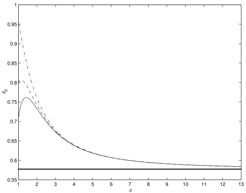
Figure 1: Downstream propagation: plot of the dependence of $z_{0}$ on $c$. (65) for CH – solid line; (66) for DP – dashed line; (67) for equation (LABEL:eq41) – dash-dotted line. All cases have a horizontal asymptote $z_{0}\rightarrow\frac{1}{\sqrt{3}}\approx 0.577$ as $c\rightarrow\infty$. The CH graph has a maximum $z_{0}\approx 0.762$ at $c\approx 1.416$; The DP graph has a maximum $z_{0}\approx 0.806$ at $c\approx 1.149$.

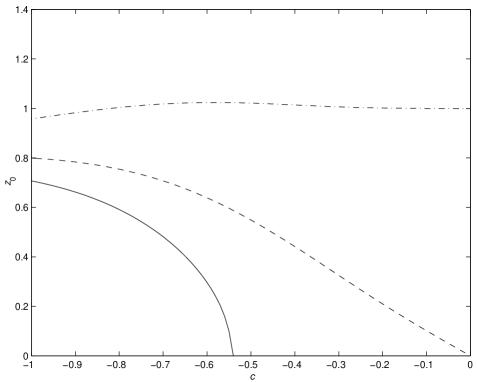
Figure 2: Upstream propagation: plot of the dependence of $z_{0}$ on $c$. (65) for CH – solid line; (66) for DP – dashed line; (67) for equation (LABEL:eq41) – dash-dotted line. The function (65) is not real for $c_{0}\leq c\leq 0$, $c_{0}\approx-0.544$; The graph of (67) has a maximum $z_{0}\approx 1.0237$ at $c\approx-0.600$.

5 Conclusions

In conclusion, CH, DP and (42) describe in a direct way (without the use of the Kodama transform) the velocity (and, consequently all related variables) of shallow water waves at depths $0.71h$, $0.80h$ and $0.96h$ correspondingly (in the absence of a shear flow), where $h$ is the depth of the undisturbed water. From a modeling point of view the advantage of the CH and DP equations over KdV consists also in the fact that they capture the wave-breaking phenomenon, cf. (Constantin 2000), (Constantin $\&$ Escher 1998) and (Zhou 2004). These equations can also be used as water wave models in the presence of an arbitrary shear flow. It is always more convenient to work with integrable equations, since their solutions are explicitly known or can be, in principle, explicitly constructed. For CH the solitons are stable patterns and thus physically recognizable, e.g. see the papers by Constantin $\&$ Strauss (2000, 2002), Constantin $\&$ Molinet (2001). The $N$-soliton solution for CH is explicitly obtained by the Inverse Scattering Method in (Constantin et al. 2006) [see also the earlier works on the CH spectral problem by Constantin (1998, 2001); Constantin $\&$ McKean, (1999)]. In parametric form the $N$-soliton solution for CH is obtained by: Johnson (2003$b$), Li $\&$ Zhang (2004), Li (2005), Parker (2004, 2005a, 2005b), Matsuno (2005$b$). Other types of explicitly known CH solutions are: multi-peakons (Beals et al., 2003), periodic solutions (Gesztesy $\&$ Holden 2003), traveling-waves (Parkes $\&$ Vakhnenko 2005), (Lenells 2005$a$). The construction of multi-soliton and multi-positon solutions for the Associated Camassa-Holm equation using the Darboux/Bäcklund transform is presented in (Schiff 1998), (Hone 1999) and (Ivanov, 2005b). The $N$-soliton solution for the DP equation was recently derived by Matsuno (2005$a$), the multi-peakon solutions for DP are obtained by Lundmark $\&$ Szmigielski (2003, 2005); the traveling waves – by Parkes $\&$ Vakhnenko (2004) and Lenells (2005$b$). There are similarities between the CH and DP equations, in a sense that they both are integrable and have a hydrodynamic derivation. However, it is interesting to notice that only CH has a geometric interpretation as a geodesic flow, cf. (Constantin $\&$ Kolev 2003), (Kolev 2004).

References

• [1]
• [2] Burns, J.C. 1953 Long waves on running water. Proc. Cambridge Phil. Soc. 49, 695–706.
• [3]
• [4] Beals, R., Sattinger, D. $\&$ Szmigielski, J. 2003 Continued fractions and integrable systems. J. Comput. Appl. Math. 153, 47–60.
• [5]
• [6] Caudrey, P., Dodd, R. $\&$ Gibbon, J. 1976 A new hierarchy of Korteweg-de Vries equations, Proc. R. Soc. London A 351, 407–422.
• [7]
• [8] Constantin, A. 1998 On the inverse spectral problem for the Camassa-Holm equation. J. Funct. Anal. 155, 352–363.
• [9]
• [10] Constantin, A. 2000 Existence of permanent and breaking waves for a shallow water equation: a geometric approach. Ann. Inst. Fourier (Grenoble) 50, 321–362.
• [11]
• [12] Constantin, A. 2001 On the scattering problem for the Camassa-Holm equation. Proc. R. Soc. Lond. A 457, 953–970.
• [13]
• [14] Constantin, A. $\&$ Escher, J. 1998 Wave breaking for nonlinear nonlocal shallow water equations. Acta Mathematica 181, 229–243.
• [15]
• [16] Constantin, A., Gerdjikov, V.S. $\&$ Ivanov R.I. 2006 Inverse scattering transform for the Camassa-Holm equation Inv. Problems 22, 2197-2207; nlin.SI/0603019.
• [17]
• [18] Constantin, A. $\&$ McKean, H.P. 1999 A shallow water equation on the circle. Commun. Pure Appl. Math. 52, 949–982.
• [19]
• [20] Constantin, A. $\&$ Kolev, B. 2003 Geodesic flow on the diffeomorphism group of the circle. Comment. Math. Helv. 78, 787–804.
• [21]
• [22] Constantin, A. $\&$ Molinet, L. 2001 Orbital stability of solitary waves for a shallow water equation. Physica 157D, 75–89.
• [23]
• [24] Constantin, A. $\&$ Strauss, W. 2000 Stability of peakons. Commun. Pure Appl. Math. 53, 603–610.
• [25]
• [26] Constantin, A. $\&$ Strauss, W. 2002 Stability of the Camassa-Holm solitons. J. Nonlinear Sci. 12, 415–422.
• [27]
• [28] Degasperis, A. $\&$ Procesi, M. 1999 Asymptotic integrability. In Symmetry and perturbation theory (ed. A. Degasperis $\&$ G. Gaeta), pp 23–37, Singapore: World Scientific.
• [29]
• [30] Degasperis, A., Holm. D.D. $\&$ Hone, A.N.W. 2002 A new integrable equation with peakon solutions. Theor. Math. Phys. 133, 1463–1474.
• [31]
• [32] Dullin, H.R., Gottwald, G.A. $\&$ Holm, D.D. 2003 Camassa-Holm, Korteweg-de Vries-5 and other asymptotically equivalent equations for shallow water waves. Fluid Dynam. Res. 33, 73–95.
• [33]
• [34] Dullin, H.R., Gottwald, G.A. $\&$ Holm D.D. 2004 On asymptotically equivalent shallow water wave equations. Physica 190D, 1–14.
• [35]
• [36] Fokas, A. $\&$ Fuchssteiner, B. 1981 Symplectic structures, their Bäcklund transformation and hereditary symmetries. Physica 4D, 821–831.
• [37]
• [38] Fokas, A. $\&$ Liu, Q. 1996 Asymptotic integrability of water waves. Phys. Rev. Lett. 77, 2347–2351.
• [39]
• [40] Gesztesy, F. $\&$ Holden, H. 2003 Soliton equations and their algebro-geometric solutions, part I: $(1+1)$ -dimensional continuous models. Cambridge studies in advanced mathematics, volume 79. Cambridge: Cambridge University Press.
• [41]
• [42] Holm, D.D. $\&$ Hone, A.N.W. 2003 Nonintegrability of a fifth-order equation with integrable two-body dynamics. Theor. Math. Phys. 137, 1459–1471.
• [43]
• [44] Hone, A. 1999 The associated Camassa-Holm equation and the KdV equation. J. Phys. A: Math. Gen. 32, L307-L314.
• [45]
• [46] Ivanov, R.I. 2005$a$ On the integrability of a class of nonlinear dispersive wave equations. Journal of Nonlinear Mathematical Physics 12, 462–468; arXiv: nlin/0606046v1 [nlin.SI]
• [47]
• [48] Ivanov, R.I. 2005$b$ Conformal properties and Bäcklund transform for the Associated Camassa-Holm equation. Phys. Lett. 345A, 235-243; arXiv: nlin/0507005v1 [nlin.SI]
• [49]
• [50] Johnson, R.S. 1997 A modern introduction to the mathematical theory of water waves, Cambridge: Cambridge University Press.
• [51]
• [52] Johnson, R.S. 2002 Camassa-Holm, Korteweg-de Vries and related models for water waves. J. Fluid Mech. 457, 63–82.
• [53]
• [54] Johnson, R.S. 2003$a$ The Camassa-Holm equation for water waves moving over a shear flow. Fluid Dyn. Res. 33, 97–111.
• [55]
• [56] Johnson, R.S. 2003$b$ On solutions of the Camassa-Holm equation. Proc. Roy. Soc. Lond. A 459, 1687–1708.
• [57]
• [58] Kaup, D. 1980 On the inverse scattering problem for the cubic eigenvalue problem of the class $\phi_{xxx}+6Q\phi_{x}+6R\phi=\lambda\phi$. Stud. Appl. Math. 62, 189–216.
• [59]
• [60] Kodama, Y. 1985 On integrable systems with higher order corrections. Phys. Lett. 107A, 245–249.
• [61]
• [62] Kolev, B. 2004 Lie groups and mechanics: an introduction. J. Nonlinear Math. Phys. 11, 480–498.
• [63]
• [64] Lenells, J. 2005$a$ Traveling wave solutions of the Camassa-Holm equation. J. Differential Equations 217, 393–430.
• [65]
• [66] Lenells, J. 2005$b$ Traveling wave solutions of the Degasperis-Procesi equation. J. Math. Anal. Appl. 306, 72–82.
• [67]
• [68] Li, Y. $\&$ Zhang, J. 2004 The multiple-soliton solutions of the Camassa-Holm equation. Proc. R. Soc. Lond. A 460, 2617-2627.
• [69]
• [70] Li, Y. 2005 Some water wave equations and integrability. J. Nonlinear Math. Phys. 12 (Suppl. 1), 466-481.
• [71]
• [72] Lundmark, H. $\&$ Szmigielski, J. 2003 Multi-peakon solutions of the Degasperis-Procesi equation. Inv. Problems 19, 1241–1245.
• [73]
• [74] Lundmark, H. $\&$ Szmigielski, J. 2005 Degasperis-Procesi peakons and the discrete cubic string. Int. Math. Res. Pap. no. 2, 53–116.
• [75]
• [76] Matsuno, Y. 2005$a$ The $N$-soliton solution of the Degasperis-Procesi equation. Inv. Problems 21, 2085–2101. arXiv: nlin/0511029v1 [nlin.SI]
• [77]
• [78] Matsuno, Y. 2005$b$ Parametric representation for the multisoliton solution of the Camassa-Holm equation. J. Phys. Soc. Japan 74, 1983–1987; arXiv: nlin/0504055v1 [nlin.SI]
• [79]
• [80] Mikhailov, A.V. $\&$ Novikov, V.S. 2002 Perturbative symmetry approach. J. Phys. A 35, 4775–4790.
• [81]
• [82] Olver, P. $\&$ Jing Ping Wang 2000 Classification of integrable one-component systems on associative algebras. Proc. London Math. Soc. 81, 566–586.
• [83]
• [84] Parker, A. 2004 On the Camassa-Holm equation and a direct method of solution I. Bilinear form and solitary waves. Proc. R. Soc. Lond. A 460, 2929-2957.
• [85]
• [86] Parker, A. 2005$a$ On the Camassa-Holm equation and a direct method of solution II. Soliton solutions. Proc. R. Soc. Lond. A 461, 3611-3632.
• [87]
• [88] Parker, A. 2005$b$ On the Camassa-Holm equation and a direct method of solution III. N-soliton solutions. Proc. R. Soc. Lond. A 461, 3893-3911.
• [89]
• [90] Parkes, E. $\&$ Vakhnenko, V 2004 Periodic and solitary-wave solutions of the Degasperis-Procesi equation. Chaos Solitons Fractals 20, 1059–1073.
• [91]
• [92] Parkes, E. $\&$ Vakhnenko, V 2005 Explicit solutions of the Camassa-Holm equation. Chaos, Solitons and Fractals 26, 1309–1316.
• [93]
• [94] Sanders, J. $\&$ Jing Ping Wang 1998 On the integrability of homogenous scalar evolution equations, J. Diff. Eq. 147, 410–434.
• [95]
• [96] Sawada, K. $\&$ Kotera, T. 1974 A method for finding $N$-soliton solutions of the KdV equation and KdV-like equation. Progr. Theor. Phys. 51, 1355–1367.
• [97]
• [98] Schiff, J. 1998 The Camassa-Holm equation: a loopgroup approach. Physica 121D, 24–43.
• [99]
• [100] Zhou, Y. 2004 Blow-up phenomenon for the integrable Degasperis- Procesi equation. Phys. Lett. 328A, 157–162.
• [101]