Rotational cooling efficiency upon molecular ionization: the case of Li${}_{2}(a^{3}\Sigma_{u}^{+})$ and Li${}_{2}^{+}(X^{2}\Sigma_{g}^{+})$ interacting with ⁴He

Abstract

The low-temperature (up to about 100K) collisional (de)excitation cross sections are computed using the full coupled-channel (CC) quantum dynamics for both Li₂ and Li${}_{2}^{+}$ molecular targets in collision with ⁴He. The interaction forces are obtained from fairly accurate ab initio calculations and the corresponding pseudo-rates are also computed. The results show surprising similarities between sizes of inelastic flux distributions within final states in both systems and the findings are connected with the structural change in the molecular rotor features when the neutral species is replaced by its ionic counterpart.

I Introduction

Lithium-bearing molecules have been a source of research interest for several years, since they may have played an important role as coolers (through rotational transitions) in the young universe (see Bodo et al. (2003) for a detailed review of the topic). Their usefulness in the study of molecular dynamics at ultralow temperatures has also been demonstrated recently in relation with their possible role in molecular formation under Bose-Einstein condensation conditions in magneto-optical traps (Cvitaš et al., 2005a; Cvitaš et al., 2007; Cvitaš et al., 2005b; Bartenstein et al., 2005). Two types of lithium dimers are studied here in relation to their collisions with ⁴He atoms: Li${}_{2}(a^{3}\Sigma_{u}^{+})$ and Li${}_{2}^{+}(X^{2}\Sigma_{g}^{+})$, hereafter simply called “neutral” and “ion”. Although they are not easily observable because of the absence of a permanent electric dipole moment, their comparative study is interesting in several respects, e.g. the change upon ionization within the full manifold of internal state transitions of the collisional behavior and the importance of the quadrupolar ($\Delta J=2$) transitions. Furthermore, although the lithium dimer could be considered the second simplest homonuclear molecule after H₂, only a few recent studies (see Minaev (2005) and references therein) have begun to give information on its chemistry, spectroscopy and collisional properties. Hence, still a lot of work has to be done to fully understand this arguably simple case. The scope of the present paper is thus to compare the dependence of collisional quantities, i.e. cross sections and rates, on changing the electronic state of the dimer target.

The paper is organized as follows: Section II outlines the computation methods and the numerical algorithm employed in this study. Section III reports the results of our scattering calculations, with an analysis of the similarities/differences between the two title systems. Section IV summarizes our conclusions.

II The computational procedure

II.1 Analytic fitting of the potential energy surfaces

The two potential energy surfaces (PES) used in the present work have already been computed from ab initio calculations carried out at the MP4 ab initio level Bodo et al. (2005). Both systems are treated here as rigid rotors, with bond lengths fixed at their equilibrium values : 4.175Å for the neutral, 3.11Å for the ion. We considered in all calculations only the dominant isotope of Li, ⁷Li. Accordingly, we used in the dynamical calculations rotational constant $B$ values of 0.2758 and 0.4971 cm^-1, respectively.
The difference in bond lengths when ionization takes place appears to be a peculiar property of the present system and is by no means a general feature of diatomic targets undergoing ionization, as shown by the data of table 1.

mol.	state	re [a0]	B [cm-1]
Li2	$X^{1}\Sigma_{g}^{+}$ lid	5.10	0.660
Li${}_{2}^{+}$	$X^{2}\Sigma_{g}^{+}$ lid	5.88 (15%)	0.4971
Li2	$a^{3}\Sigma_{u}^{+}$ lid	7.89 (55%)	0.2758
Na2	$X^{1}\Sigma_{g}^{+}$ Ho et al. (2000)	5.82	-
Na${}_{2}^{+}$	$X^{2}\Sigma_{g}^{+}$ Patil and Tang (2000)	6.8 (17%)	-
Na2	$a^{3}\Sigma_{u}^{+}$ Ivanov et al. (2003)	9.76 (68%)	-
K2	$X^{1}\Sigma_{g}^{+}$ J. et al. (1987)	7.41	-
K${}_{2}^{+}$	$X^{2}\Sigma_{g}^{+}$ Patil and Tang (2000)	8.3 (12%)	-
K2	$a^{3}\Sigma_{u}^{+}$ Jong et al. (1992)	10.91 (47%)	-
H2	X${}^{1}\Sigma$	1.40	60.85
H${}_{2}^{+}$	X${}^{2}\Sigma_{g}^{+}$	1.98	30.20
O2	X${}^{3}\Sigma_{g}^{-}$	2.29	1.438
O${}_{2}^{+}$	X${}^{2}\Pi_{g}$	2.12	1.691
Ne2	X${}^{1}\Sigma_{g}^{+}$	5.86	0.17
Ne${}_{2}^{+}$	X${}^{2}\Sigma_{u}^{+}$	3.31	0.55

Table 1: Comparison of molecular parameters for homonuclear neutral and ionic molecules in their electronic ground and first excited states. Figures in parenthesis give the percentage lengthening of the bond with respect to the ${}^{1}\Sigma$ reference state. Numbers, if not directly referenced, are taken from the NIST diatomic database nis .

It is interesting to understand why the bond distances become longer in the case of the ionic doublets and even more so for the neutral triplets. The changes of core orbitals along the alkali metal sequence are balanced by the increase in atomic numbers that create more attractive Coulomb wells around the nuclei. Thus, the outer electrons (one or two) play a very similar role in all three systems, going from Li dimers to K dimers. The crucial difference thus comes from the Pauli repulsion occurring between the outer electrons of the ${}^{3}\Sigma$ case (they have aligned spins), which is even stronger than the additional repulsive contribution among core electrons and the single outer one that is a consequence of the reduction of the screening of nuclear charges caused by the ionization process. Such an effect is not observed for the non-alkali dimers reported in table 1, where we observe always bond contraction after molecular ionization processes, except for the H₂ dimer which, with only two bound electrons, is another system which follows the alkali metal behavior. In conclusion, the two title systems show very marked bond lengthening both upon ionization and on spin stretching.

To solve the close coupling equations, it is necessary to generate the matrix elements of the coupling potential between the basis of asymptotic functions. Since the latter are given by Legendre polynomials, we fit the potential as follows

$$V(R,\theta|r_{eq})=\sum_{\lambda}V_{\lambda}(R|r_{eq})P_{\lambda}(\cos(\theta))$$ (1)

where $R$ is the intermolecular distance (distance from the center of mass of the dimer to the atom), $r_{eq}$ is the diatomic rigid rotor bond distance, $\theta$ is the angle between the dimer and the intermolecular vector, $P_{\lambda}$ are the Legendre polynomials, and $V_{\lambda}$ are the radial coefficients. The latter are the potential coupling coefficients which shall be employed in the scattering equations. We thus need to evaluate them at any $R$, with $\lambda$ large enough for the expansion to reach a preselected precision. In practice, we solve it over a discrete radial grid, and then interpolate the $V_{\lambda}$ with cubic splines, further extrapolating them with exponentials at short range and a two-term inverse power law at long range.

Both systems, although showing different potentials, are strongly anisotropic in the short range region: for some chosen value of $R$, the potential can therefore be for different angles either strongly attractive or repulsive by several thousands cm^-1. This feature makes it numerically difficult when trying to generate the radial coefficients. A method has been applied (e.g. see Wernli et al. (2007)) which permits to circumvent this difficulty: at a given $R$ value, we first truncate the potential up to a few thousand cm^-1and then apply a smoothing function to this truncated potential to avoid the Gibbs oscillations that would inevitably come when fitting directly the truncated potential. Finally, we fit this functional of the potential with a weighting strategy, giving more relevance (thus higher fitting precision) to the low-energy parts of the potential in comparison with the more repulsive regions. Thus, we optimized the fitting parameters for the low-energy dynamics which we intend to study by finally getting potential fits with a precision of better than 2 cm^-1 for $V\lesssim 800$ cm^-1.

II.2 The quantum dynamics

We briefly recall here the equations of the close-coupling formalism we have employed. Using the center of mass frame, the time-independent Schrödinger equation writes

$$\left(T_{r}+T_{R}+v_{mol}(r)+V_{I}(r,R,\theta)-E\right)\Psi^{JM}(\vec{R},\vec{r})=0$$ (2)

where

$$T_{r} = -\frac{1}{2m}\nabla_{r}^{2}\quad{\rm and}$$ (3)

$$T_{R} = -\frac{1}{2\mu}\nabla_{R}^{2}$$ (4)

where $m$ is the reduced mass of the diatom and $\mu$ that of the complex. E is the total energy. The interatomic distance of the diatom is denoted $r$, $R$ is the distance between the colliding atom and the diatom center of mass and $\theta$ is the angle between $\vec{R}$ and $\vec{r}$. The $v_{mol}$ term is the potential of the isolated diatom and $V_{I}(r,R,\theta)$ is the interaction potential, eq. (1). To solve equation (2), the $\Psi^{JM}(\vec{R},\vec{r})$ is expanded on a basis of asymptotic eigenfunctions of the isolated partners, which are treated here as rigid rotor targets ($\overline{r}=\overline{r}_{eq}$ for each of them) and therefore $\overline{r}_{eq}$ disappears as an explicit variable of the present problem.

$$\Psi^{JM}(\vec{R},\hat{r}_{eq})=\frac{1}{R}\sum_{n}C_{n}(R)\phi_{n}(\hat{R},\hat{r}_{eq})$$ (5)

where the channel function for channel $n\equiv(jl\,;JM)$ is given by

$$\phi_{n}(\hat{R},\hat{r}_{eq})=\sum_{m_{j},m_{l}}(j,l,J|m_{j},m_{l},M)Y^{j}_{m_{j}}(\hat{r}_{eq})Y^{l}_{m_{l}}(\hat{R})$$ (6)

The quantum number for rotation is denoted by $j$ and $l$ is the orbital angular momentum of the atom with respect to the diatom. $J$ is the total angular momentum ($\vec{J}=\vec{j}+\vec{l}$), $M$ is the projection of $J$ on the laboratory frame fixed $z$ axis, and $(j,l,J|m_{j},m_{l},M)$ is a Clebsch-Gordan coefficient. Solving the present problem is thus equivalent to determining the expansion coefficients $C_{n}(R)$. Multiplying the l.h.s. of eq. (2) by $\phi_{i}$ and integrating over $\hat{R}$ and $\hat{r}$, then using eq. (5) and (6), we find

$$\left(\frac{d^{2}}{dR^{2}}-\frac{l_{i}(l_{i}+1)}{R^{2}}+2\mu E_{i}\right)C_{i}(R)=2\mu\sum_{n}C_{n}(R)\left<\phi_{i}|V_{I}|\phi_{n}\right>$$ (7)

where $E_{i}=E-\epsilon_{j}$ is the initial kinetic energy (the collision energy) and $l_{i}$ is the angular orbital momentum in the $i$th channel. $\epsilon_{j}=Bj(j+1)$ is the rotational energy of the target. We obtained a second-order differential equation to be solved for each $i$, thus a set of equations for the $C_{i}(R)$ coefficients, called coupled channel (CC) equations.

The radial coefficients $V_{\lambda}(R)$ hence appear in the sum of terms on the r.h.s. of eq. (7),as the weighting radial terms of the potential times the angular coupling terms generated by the potential anisotropy between rotational asymptotic channels $\left<\phi_{i}|P_{\lambda}|\phi_{n}\right>$. We thus know that the angular dependence of the interaction applies, during collisions, a torque to the rotating target which acts over the radial range of action of each $V_{\lambda}(R)$ coefficient.

To solve the CC equations we used the code developed in our group, where the propagator was given by a log-derivative algorithm at short range and by the modified variable-phase propagator at long range, as discussed by Martinazzo et al. (2003).

The initial tests for the neutral showed that the inelastic cross sections would exhibit very few and fairly small resonance features. Accordingly, we chose a rather sparse energy grid corresponding to a minimum of 50 energies for the highest initial $j$, this number increasing with decreasing initial $j$. The energies were chosen to be mainly distributed around the expected isolated resonance energies, in order to obtain a good description of these features.
The propagators parameters were accurately tested at two representative energies and the integration was thus carried out using the Log-Derivative propagator between 2 and 30 Å (in 500 steps), and our Modified Variable Phase propagator between 30 and 200 Å.
The rotational basis chosen covered a range of more than 100 cm^-1 for the closed channels at all energies and it proved to be necessary to compute partial cross-sections up to a total angular momentum of 35$\hbar$ in order to get a satisfactory convergence (around 5%), at the higher rotational transitions.
Our results were further tested at a few energies using an entirely different code by Hutson and Green (see ref. Hutson and Green (1994)). We found an excellent agreement between the two codes, with differences remaining always under 1%.

When computing rotational transitions for the ion the larger potential depth induces a much richer resonance structure. We consequently adopted a more dense energy grid and a larger rotational basis. The minimum number of energy points for all transitions is here about 100 in the energy range of 1-100 cm^-1 and we also computed a few points up to 600 cm^-1 to further ensure numerical convergence of our rate coefficients (see below for additional details). For the ion, we used more or less the same propagation parameters as for the neutral, while just switching from one propagator to the other at an earlier distance of 15 Å. We also used at all energies a rotational basis equivalent to at least a range of 300 cm^-1 spanned by the energies of the closed channels. The maximum total angular momentum needed below 100 cm^-1 was of $\sim$45$\hbar$.

For both systems the detailed balance on the cross sections gave an excellent agreement at all energies, the largest error coming at low energies, with differences around 5%. This permits us to state that our final cross sections are numerically converged within that error value.

Since the main scope of this paper is the comparison of rotational (de)excitation behavior of the two systems, the spin coupling effects (spin-spin and spin-rotation) are neglected and both systems are treated as pseudo-${}^{1}\Sigma$ targets. This approximation is fully justified at our energies, since spin coupling constants are small for both systems. According to Kurls’s formula (e.g. see ref. Lefebvre-Brion and Robert (1986)) and using the data provided to us by E. Yurtsever (private communication) obtained via the Gaussian code (e.g. see ref. Frisch et al. (1998)), we find that the spin-rotation constants are respectively $4.8\ 10^{-5}$ and $4.3\ 10^{-5}$ cm^-1 for the neutral and the ion. We have nonetheless performed a few numerical tests with the correct coupling calculations at several energies between 1 and 30 cm^-1, and for both systems we found that the inclusion of the spin-rotation coupling has only a small effect at the energies we considered. If we sum over final spin states, the value of a given rotational transition, in fact, does not depend on the initial choice by more than 5%. Furthermore, the difference between the summed cross section and its value from the pseudo-${}^{1}\Sigma$ calculation is less than $10$%. At all the energies of this range, moreover, the systems preferentially stay in their original spin state, this preference varying from a factor of $\sim 1.5$ to more than 10. These results confirm the validity of the pseudo-singlet approximation employed in our extensive calculations reported below.

III Results and discussion

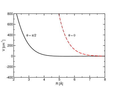
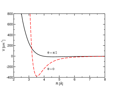
Figure 1: Potential energy curves for neutral and ionic Li₂ interacting with ⁴He, as a function of intermolecular distance for the collinear ($\theta=0$) and perpendicular ($\theta=\pi/2$) relative orientations. Left panel: Li₂; right panel: Li${}_{2}^{+}$. The global minimum of Li₂-He interaction is -2.3 cm^-1.

Figure 1 shows the potential energy curves resulting from our fit for both systems and reports their minimum orientations. The two surfaces markedly differ in several points: the potential well depth is more than a hundred times deeper in the case of the ion and the repulsive walls at short range do not have the same slope, neither the same location. But two facts are nonetheless common to both molecular partners: (i) the presence of an attractive interaction in the medium to long range region and a strongly repulsive wall when approaching at short range each molecule and (ii) the presence of only two dominant multipolar potential terms at long range, i.e. $V_{0}(R)$ and $V_{2}(R)$. For the ion, they correspond respectively to the charge-induced dipole and charge-induced quadrupole interactions. For the neutral partner, we have instead the isotropic and anisotropic part of the dispersion interaction, respectively. Both terms for the neutral are smaller than for the ion. Moreover, the $V_{0}$ vanishes more rapidly for the neutral. In conclusion, the neutral triplet state exhibits “softer” repulsive regions than the more compact ionic doublet.

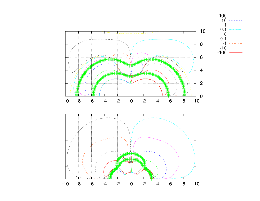
Figure 2: Torques ($\partial V/\partial\theta$) isolines for the Li₂ (upper panel) and Li${}_{2}^{+}$ (lower panel) as a function of the cartesian coordinates $x$ and $y$, in Å. The zero potential isolines those at 200 cm^-1 are given by thicker lines. The energy isolines scale is logarithmic: -100, -10, -1, -0.1, 0, 0.1, 1, 10, 100 cm^-1.

Figure 2 shows the computed “potential torques” ($\partial V/\partial\theta$) for both systems, using the same unit scale and as a function of the $x$ and $y$ cartesian coordinates. As seen before with the potential curves, the computed torques have very different ranges of action, although they have in common that the most efficient angular coupling for both systems is in the range of $\theta=30-40^{o}$. From the shape of the angular torques, combined with the features of figure 1, we see that the helium atom can get closer to the molecular partner in the case of the neutral (its repulsive wall is less steep) than in the ionic case, so that the overall torques sampled at a given collision energy are of the same order of magnitude for both systems in the sense that the weaker torque applied by the incoming He atom to the neutral partner has a much larger range of action during collision than in the case of the stronger torque applied to the ionic partner. If we combine this finding with the reduced energy gaps between rotor states of the triplet when is compared with the ion, we see that the neutral interaction, albeit weaker, becomes just as efficient in exciting rotations as the corresponding ionic target.

Figure 3 shows some illustrative results obtained for the cross sections. The most surprising finding is that at collision energies of a few cm^-1 above threshold the deexcitation cross sections are of the same order of magnitude for both systems. One would have expected that the much deeper potential well depth and the greater strength of the long-range forces would cause larger cross sections for the ion. On the other hand, the foregoing discussion on the range of action of the rotational torques acting during collision provides a structural explanation for the size similarities between cross sections. We should also note that ref. Wernli et al. (2007) has already shown that for large enough bond distances the collisional behavior is dominated by the geometry of the target molecule and classical calculations provide good agreement with quantum results. Consequently, we should expect that a classical approach to rotational cooling may also work reasonably well for the two title systems of the present work.
One should also note here that the oscillatory structures are much richer in the case of the ion, occurring up to 50 cm^-1 above threshold. It is hard to decide whether these structures are due to resonant features or to background interference effects without a proper analysis of the corresponding S-matrix elements. As we consider such a study, because of the absence of experimental data, outside the scope of this paper, we are not discussing these features any more. For the neutral, on the other hand, only one small feature in the cross sections appears, associated with the opening of the first rotational channel. Apart from such low-energy findings, the behavior of all cross sections is largely featureless as the energy increases. In both cases, rotational deexcitation is a more favorable process when starting from higher $j$ values. Hence, rotational excitation is expected to be easier from low $j$ initial states. As noted before, the largest difference between the two systems comes at low energies, where the strong increase of cross sections is much more marked in the case of the ion as the energy decreases: clearly, at low energies, the systems are more sensitive to the outer potential details like well depth and long range forces, the latter dominating the threshold behavior in the ionic system.

If we further define a quantity we shall call the pseudo-rates $K$ as $K_{j\to j^{\prime}}(E)=\sigma_{j\to j^{\prime}}v(E)$, where $v(E)$ is the velocity associated to the initial collision energy E : $v=\sqrt{2E/\mu}$ , we note that these quantities are generally a good approximation of true Boltzmann rates when the cross sections are nearly featureless and smoothly vary with temperature, given as $E=kT$ in the pseudo-rates. As discussed for the data shown by figure 3, this is what occurs in the present calculations.

To assess the reliability of this approximation, we also computed temperature dependent rates for some transitions and in the range of 10-100K. In figure 4 we therefore report the summed-over-final-states Boltzman rates and the pseudo-rates, $\sum_{j^{\prime}\leq 10}K_{j\to j^{\prime}}$, as a function of temperature for the two systems. Three main features are illustrated by the plots: (i) on all four panels, we see that the pseudo-rates are a very good approximation to the true Boltzmann-integrated rates. The size and temperature dependence are largely the same, the main difference being that the Boltzman integration smooths out the curves and makes the resonances patterns disappear while it is not the case with the pseudo-rates: the average precision of this pseudo-rate approximation can furthermore be estimated to be around 20%; (ii) outside the resonance structure shown by the ion, we see that, the global inelastic behavior of these pseudo-rates is nearly the same for both molecular partners, the principal difference showing up at low energy, as was the case for cross sections; (iii) one further difference between the two systems is to be found in the elastic rates/cross sections, which turn out to be about twice as big for the ion as for the neutral. Thus, we can say that the overall flux redistribution after collisions is dominated by elastic processes in the ionic case, while for the neutral, the sizes of elastic and inelastic flux redistributions are nearly equal.

IV Conclusions

We have computed rotationally inelastic cross sections and pseudo rates for the lithium dimer in two different electronic states, treated as pseudo-${}^{1}\Sigma$ molecules, interacting with a helium atom in the range of energy between 1 and 100 cm^-1. We found the unexpected result that, except for the low energy behavior and the resonance structures present in the ionic case, the inelastic cross sections and rates are rather close between neutral and ionic partners although the potential well depths, the repulsive walls and the long range behaviors are different in the two cases. The explanation comes from the fact that at these energies, the collisional behavior is dominated by the geometry effects; in other words, the dynamically accessible torques at a given energy for a given transition are similar for both systems. The elastic cross sections and rates are however much more different, with a factor of 2 in favor of the ion, as one should expect.

The present calculations therefore help us to shed more light on the role played by molecular features in low energy inelastic scattering processes, in the sense that the presence of either neutral or ionized lithium dimers in the gaseous medium would result, in both cases, in comparable cooling efficiency for scattering with ⁴He as a buffer gas. On the other hand, the differences in elastic cross sections suggest that the ionic partner would yield much larger momentum transfer cross sections with the same partner gas and would therefore undergo more rapidly a translational cooling process by sympathetic collisions (e.g. see Bodo and Gianturco (2006)).

V Acknowledgments

The financial support of the University of Rome “La Sapienza” Research Committee and of the CASPUR Computing Consortium is gratefully acknowledged. One of us (M.W.) thanks the Department of Chemistry of “La Sapienza” for the award of a Research Fellowship.

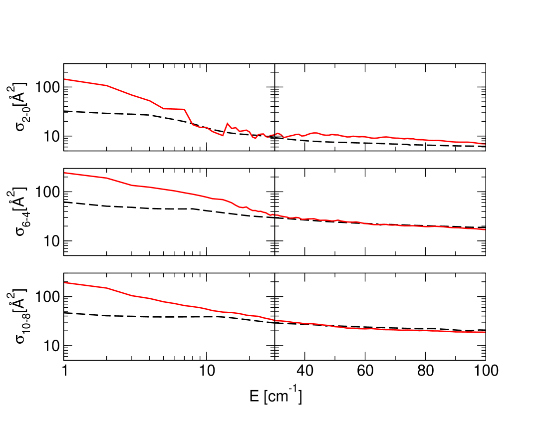
Figure 3: Computed rotational deexcitation cross sections for both systems as a function of collision energy. The calculations for the ion are given by solid lines, while those for the neutral are given by dashes. The three transitions represented are, from top to bottom, those involving the following levels: 2-0, 6-4, 10-8. The energy scale is logarithmic between 1 and 30 cm^-1, then linear at higher energy.

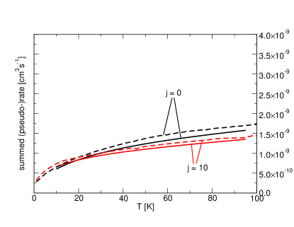
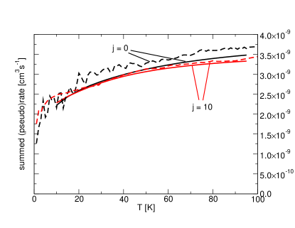
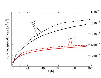
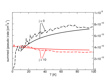
Figure 4: Rotationally summed (pseudo-)rates for the excitation (from j=0) and de-excitation (from j=10) processes. Left panels: neutral, right panels.: ion. Two different initial states are considered by including or excluding the elastic cross sections. Pseudo-rates are represented using dashes, while real rates are given by full lines. The upper panels are the sums including the elastic cross sections, while the lower panels plot the sums without the elastic cross sections.

References

- Bodo et al. (2003) E. Bodo, F. A. Gianturco, and R. Martinazzo, Phys. Rep. 384, 85 (2003).
- Cvitaš et al. (2005a) M. T. Cvitaš, P. Soldán, J. M. Hutson, P. Honvault, and J.-M. Launay, Phys. Rev. Lett. 94, 033201 (2005a).
- Cvitaš et al. (2007) M. T. Cvitaš, P. Soldan, J. M. Hutson, P. Honvault, and J.-M. Launay, ArXiv Physics e-prints (2007), eprint physics/0703136.
- Cvitaš et al. (2005b) M. T. Cvitaš, P. Soldán, J. M. Hutson, P. Honvault, and J.-M. Launay, Phys. Rev. Lett. 94, 200402 (2005b).
- Bartenstein et al. (2005) M. Bartenstein, A. Altmeyer, S. Riedl, R. Geursen, S. Jochim, C. Chin, J. H. Denschlag, R. Grimm, A. Simoni, E. Tiesinga, et al., Phys. Rev. Lett. 94, 103201 (2005).
- Minaev (2005) B. Minaev, Spectrochimica Acta Part A 151, 790 (2005).
- Bodo et al. (2005) E. Bodo, F. A. Gianturco, E. Yurtsever, and M. Yurtsever, Mol. Phys. 103, 3223 (2005).
- (8) Data from our calculations.
- Ho et al. (2000) T.-S. Ho, H. Rabitz, and S. G., J. Chem. Phys. 112, 6218 (2000).
- Patil and Tang (2000) S. H. Patil and K. T. Tang, J. Chem. Phys. 113, 676 (2000).
- Ivanov et al. (2003) V. S. Ivanov, V. B. Sovkov, and L. Li, J. Chem. Phys. 118, 8242 (2003).
- J. et al. (1987) H. J., U. Schuhle, F. Engelke, and C. D. Caldwell, J. Chem. Phys. 87, 45 (1987).
- Jong et al. (1992) G. Jong, L. Li, T.-J. Whang, W. C. Stwalley, J. A. Coxon, M. Li, and A. M. Lyyra, J. Mol. Spec. 155, 115 (1992).
- (14) Data from NIST Standard Reference Database 69 June 2005 Release: NIST Chemistry WebBook.
- Wernli et al. (2007) M. Wernli, L. Wiesenfeld, A. Faure, and P. Valiron, A&A 464, 1147 (2007).
- Martinazzo et al. (2003) R. Martinazzo, E. Bodo, and F. Gianturco, Comp. Phys. Com. 151, 187 (2003).
- Hutson and Green (1994) J. M. Hutson and S. Green, molscat computer code, version 14 (1994), distributed by Collaborative Computational Project No. 6 of the Engineering and Physical Sciences Research Council (UK).
- Lefebvre-Brion and Robert (1986) H. Lefebvre-Brion and W. Robert, Perturbations in the Spectra of Diatomic Molecules (Academic Press, 1986).
- Frisch et al. (1998) M. Frisch, G. Trucks, and H. e. a. Schlegel, Gaussian 98 (Revision A.1x) (1998), gaussian, Inc., Pittsburgh, PA.
- Bodo and Gianturco (2006) E. Bodo and F. A. Gianturco, Int. Rev. Phys. Chem. 25, 313 (2006).