Nonlinear transport of Bose-Einstein condensates through mesoscopic waveguides

Abstract

We study the coherent flow of interacting Bose-condensed atoms in mesoscopic waveguide geometries. Analytical and numerical methods, based on the mean-field description of the condensate, are developed to study both stationary as well as time-dependent propagation processes. We apply these methods to the propagation of a condensate through an atomic quantum dot in a waveguide, discuss the nonlinear transmission spectrum and show that resonant transport is generally suppressed due to an interaction-induced bistability phenomenon. Finally, we establish a link between the nonlinear features of the transmission spectrum and the self-consistent quasi-bound states of the quantum dot.

I Introduction

The development of microscopic trapping potentials for ultracold atoms has lead to a number of fascinating experiments probing the behaviour of Bose-Einstein condensates on mesoscopic length scales. Examples include the realization of a Josephson weak link between two condensates in a double well potential AnkO05PRL , the measurement of interference and phase coherence between two spatially separate condensates ShiO05PRA ; SchO05NP , as well as the diffraction of a condensate from a magnetic lattice GueO05PRL . A convenient setup for such experiments is provided by “atom chips” FolO00PRL where microscopic confinement potentials are created with the magnetic field that is induced by current-carrying electric wires mounted on top of the chip surface. This technique does not only allow one to produce microtraps, but also to create waveguide geometries for cold atoms that can be rather flexible, and thereby opens the way to explore transport properties of cold atomic gases. Early experiments on atom chips did indeed focus on the propagation of a Bose-Einstein condensate along such a magnetic waveguide, where the condensate was transported in a controlled way by means of time-dependent magnetic fields HaeO01N or accelerated along the guide by means of a field gradient OttO03PRL .

The possibility to create such waveguides for cold atoms have stimulated a number of theoretical investigations on the transport physics of interacting matter waves, with particular emphasis on possible analogies with mesoscopic phenomena in the electronic context. This started with the attempt to define an atomic analog of Landauer’s quantization of the conductance ThyWesPre99PRL , and was continued by the generalization of the “Coulomb blockade” phenomenon to cold bosonic atoms propagating through a quantum-dot-like potential CarLar99PRL ; Car01PRA . More recent studies, which are based on an elaborate framework for the description of scattering processes of Bose-Einstein condensates (to be described in this article), include the nonlinear resonant transport of a condensate through atomic quantum dots PauRicSch05PRL ; RapWitKor06PRA , the manifestation or absence of Anderson localization in the transport through disorder potentials PauO05PRA ; Pau07PRL , as well as the transport of solitons through disorder BilPav05PRL . For their experimental realization, these transport processes would require a coherent quasi-stationary flow of Bose-Einstein condensed atoms in the waveguide, which was recently realized in the context of optical guides Gue06PRL using the principle of “atom lasers” BloHaeEss99PRL .

From the theoretical point of view, the main complication in the description of a quasi-stationary scattering process of a Bose-Einstein condensate obviously comes from the presence of the atom-atom interaction. In leading order, the effect of this interaction is included in a nonlinear term in the Schrödinger-like Gross-Pitaevskii equation for the condensate wavefunction. In presence of a waveguide potential, providing a harmonic confinement in two (transverse) spatial dimensions and permitting free motion along the third (longitudinal) dimension, an adiabatic treatment of the transverse degrees of freedom allows one to describe the evolution of the condensate by means of an effective one-dimensional Gross-Pitaevskii equation as long as the confinement of the waveguide is sufficiently strong (such that the condition for the “1D mean-field regime” is satisfied MenStr02PRA ). This one-dimensional nonlinear wave equation does permit stationary solutions corresponding to condensates that propagate with finite velocity along the axis of the guide LebPav01PRA . As was shown by Leboeuf and Pavloff, these solutions can then be used in order to construct scattering wavefunctions of the condensate (with the appropriate outgoing boundary condition) in presence of finite-range perturbation potentials in the waveguide LebPavSin03PRA .

In contrast to the linear Schrödinger equation, the knowledge of stationary scattering states alone does not necessarily permit the prediction of the outcome of a given propagation experiment with Bose-Einstein condensates. This is not only the case for the propagation of finite wave packets (which obviosly cannot be decomposed into individual scattering eigenstates, due to the absence of the superposition principle in the Gross-Pitaevskii equation), but applies also to adiabatic injection processes as performed in Ref. Gue06PRL , where the waveguide is gradually filled with matter waves. Clearly, if such an adiabatic process leads to a quasi-stationary flow of the condensate (which actually need not be the case, as we pointed out in Ref. PauO05PRA ), the corresponding scattering state necessarily satisfies the stationary Gross-Pitaevskii equation. However, not every scattering eigenstate of this nonlinear Schrödinger equation can eventually be populated in this way: due to the nonlinearity, the eigenstates in the waveguide can be dynamically unstable, which means that they would disintegrate in the course of time evolution as a consequence of small deviations. Such dynamical stability properties cannot easily be inferred from the stationary Gross-Pitaevskii equation. Another nontrivial problem is, as we shall explain below, the determination of the incident flux of atoms that is associated with a given stationary scattering state. This information is required in order to establish the connection to a given propagation experiment (where the incident current is typically under much better control than the net current during the propagation) and to determine the transmission coefficient of the scattering state.

In view of these complications, it seems advisable to study waveguide scattering of Bose-Einstein condensates within the framework of the time-dependent Gross-Pitaevskii equation. While the straightforward numerical simulation of wave packet propagation processes is hardly feasible in the limit of spatially broad and energetically narrow wave packets (which would be required, e.g., for studying the energy-resolved transmission through atomic quantum dots), it is possible to directly simulate the quasi-stationary injection process from an external reservoir of Bose-Einstein condensed atoms into the waveguide, as it was experimentally performed in Ref. Gue06PRL . Assuming that this reservoir is sufficiently large such that the effect of the back-action from the waveguide can be neglected, the dynamics in the waveguide is effectively described by an inhomogeneous Gross-Pitaevskii equation, which contains a source term that models the input of matter waves from the reservoir. This inhomogeneous Schrödinger-like equation can be efficiently integrated with standard finite-difference methods, using absorbing boundary conditions in order to avoid artificial backreflections from the ends of the numerical grid. Typically one would start with vanishing condensate density in the guide, and then time-integrate the equation while adiabatically increasing the source amplitude from zero up to a given maximal value. Clearly, this approach is rather close to the realistic experiment. By construction, it automatically yields, at the end of the propagation, scattering states that are dynamically stable (provided the flow remains quasi-stationary during the integration), and it allows in a natural way to determine the transmission of those states. We have successfully applied this approach to the transport of Bose-Einstein condensates through quantum-dot-like double barrier potentials PauRicSch05PRL and through one-dimensional disorder potentials PauO05PRA .

The present paper is devoted to the detailed description of this time-dependent approach to nonlinear waveguide scattering of a Bose-Einstein condensate, and to its relation with the existence of stationary scattering states of the condensate. To this end we briefly review in Sec. II the so called 1D mean-field regime, set up the theoretical framework to study transport and scattering processes, and introduce concepts that allow to define transmission and reflection coefficients for stationary scattering states that are solutions of a nonlinear wave equation. In Sec. II.3, the numerical method that is based on integrating the time-dependent Gross-Pitaevskii equation in presence of a source term is explained. As a first application, the transmission spectrum of the condensate flow through a quantum point contact consisting of a single potential barrier in the waveguide is discussed in Sec. II.4. In Sec. III we investigate the transport through a symmetric double barrier potential and we show in III.1 that the transmission spectrum exhibits an interaction induced suppression of resonant transport. Finally, in Sec. III.2, we develop an analytical description of the transport problem through the double barrier potential in terms of internal quasi-bound states. This establishes a clear link between the nonlinear signatures of the transmission spectrum and the self-consistent quasi-bound states of the quantum dot.

II Mean-field approach to transport of condensates

In the following we consider a coherent beam of Bose-Einstein condensed atoms at zero temperature, propagating through a cylindrical waveguide with a finite-range scattering potential, given, e.g., by a constriction acting as a barrier potential for the beam. One of the aims of this work is to develop new methods to describe such propagation processes based on the Gross-Pitaevskii mean-field theory PitStribook ; DalO99RMP . The mean-field dynamics of a dilute condensate can be described in terms of a macroscopic order parameter, the condensate wave function $\Psi(\vec{r},t)$, which obeys the nonlinear Gross-Pitaevskii equation CasDum96PRL

$$i\hbar\frac{\partial}{\partial t}\Psi(\vec{r},t)=\left[-\frac{\hbar^{2}}{2m}\Delta+V(\vec{r})+U_{0}|\Psi(\vec{r},t)|^{2}\right]\Psi(\vec{r},t).$$ (1)

Low-energy scattering processes between two atoms in the condensate are predominately described by the contribution from s-wave scattering and lead to the nonlinear term $U_{0}|\Psi(\vec{r},t)|^{2}$. Here $U_{0}=4\pi\hbar^{2}a_{s}/m$ is the interaction strength which is determined by the s-wave scattering length $a_{s}$ and the mass $m$ of the condensed bosons. The term $V(\vec{r})$ in Eq. (1) is the external trapping potential experienced by the atoms. For the sake of definiteness we consider the experimentally relevant case of a condensate in a cylindrical harmonic waveguide with an additional scattering potential that is induced along the guide. Let $x$ be the coordinate along the axis of the guide and $r\equiv\sqrt{x^{2}+y^{2}}$ the cylindrical radius associated with the transverse coordinates, then we assume $V(\vec{r})$ to be of the form

$$V(\vec{r})=\frac{1}{2}m\omega^{2}r^{2}+V_{||}(x).$$ (2)

Here, the first term on the right-hand side is the transverse harmonic confinement of the guide with trapping frequency $\omega$ and $V_{||}(x)$ is the scattering potential parallel to the axis of the guide. $V_{||}(x)$ could, e.g., consist of a single barrier that acts as a constriction for the condensate flow. Such a barrier can, for instance, be induced by irradiating a strongly focused blue-detuned laser beam onto the waveguide.

II.1 1D mean-field regime

In this subsection we derive an effective one-dimensional version of the Gross-Pitaevskii equation which is particularly suited to describe condensates in elongated waveguide structures. To this end, we adopt the adiabatic approximation method outlined in Refs. JacKavPet98PRA ; MenStr02PRA ; LebPav01PRA , where the condensate wave function can be cast into the form

$$\Psi(x,r)=\psi(x,t)\phi(r,n).$$ (3)

Here, $\phi$ is the equilibrium ground state wave function for the transverse motion, normalized to unity

$$\int d^{2}r|\phi|^{2}=1,$$ (4)

$\psi(x,t)$ describes the longitudinal motion, and the density per unit of longitudinal length is given by

$$n(x,t)\equiv\int d^{2}r|\Psi|^{2}=|\psi(x,t)|^{2}.$$ (5)

We remark that this adiabatic ansatz involves a local density approximation, in the sense that one assumes that the transverse motion depends solely on the local condensate density $n(x,t)$ at position $x$. It was pointed out in Ref. JacKavPet98PRA that this approximation is justified if the transverse scale of the density variation is much smaller than the longitudinal one. This regime is certainly reached when the scale of variation of the longitudinal potential $V_{||}(x)$ is considerably larger than the harmonic oscillator length $a_{\perp}=\sqrt{\hbar/(\omega m)}$ of the radial transverse confinement.

Inserting the ansatz (3) into the Gross-Pitaevskii equation (1) yields

$$i\hbar\phi\frac{\partial}{\partial t}\psi = -\phi\frac{\hbar^{2}}{2m}\psi+\psi\left[-\frac{\hbar^{2}}{2m}\left(\frac{\partial^{2}}{\partial r^{2}}+\frac{1}{r}\frac{\partial}{\partial r}\right)+\right.$$ (6)

$$\left.+\frac{1}{2}m\omega^{2}r^{2}+U_{0}n(x,t)|\phi|^{2}\right]\phi.$$

We can identify the term in the square brackets as the effective Hamiltonian $H_{T}$ for the transverse degree of freedom, acting on the wave function $\phi$,

$$H_{T}\phi=\epsilon(n)\phi.$$ (7)

The energy $\epsilon(n)$ associated with the transverse state $\phi$ depends parametrically on the longitudinal density $n$. Thus, we obtain a pair of equations, one for the transverse, and one for the longitudinal dynamics of the condensate,

$$\epsilon(n)\phi = \left[-\frac{\hbar^{2}}{2m}\left(\frac{\partial^{2}}{\partial r^{2}}+\frac{1}{r}\frac{\partial}{\partial r}\right)+U_{0}n(x,t)|\phi|^{2}\right.$$ (8)

$$\left.+\frac{1}{2}m\omega^{2}r^{2}\right]\phi,$$

$$i\hbar\frac{\partial}{\partial t}\psi = \left[-\frac{\hbar^{2}}{2m}\frac{\partial^{2}}{\partial x^{2}}+V_{\|}(x)+\epsilon(n(x,t))\right]\psi.$$ (9)

Eq. (9) is an effective one dimensional wave equation for the longitudinal order parameter $\psi$ which is particularly suited to describe a condensate in non-uniform waveguides. This regime is often denoted as the 1D mean-field regime MenStr02PRA .

It remains to determine $\epsilon(n)$. In the following, we assume that $\phi$ is the energetic ground state of $H_{T}$. In the so-called low density limit, $a_{s}n\ll 1$, the nonlinear term $U_{0}n|\phi|^{2}$ in Eq. (8) is a small perturbation and a first-order perturbative solution of Eq. (8) yields

$$\epsilon(n)=\epsilon_{0}+U_{0}\langle\phi\left||\phi_{0}|^{2}\right|\phi_{0}\rangle=\epsilon_{0}+2\hbar\omega a_{s}n,$$ (10)

where $\epsilon_{0}=\hbar\omega$ is the eigenenergy of the ground state $\phi_{0}$ of the unperturbed transverse Hamiltonian ($\epsilon_{0}$ is a constant energy shift which we drop in the following). In the opposite large density limit, $a_{s}n\gg 1$, the kinetic energy term in Eq. (9) can be neglected, and the so called Thomas-Fermi approximation holds for the transverse wave function DalO99RMP , yielding

$$\phi_{TF}=\frac{1}{U_{0}\sqrt{n}}\sqrt{\epsilon(n)-V_{\perp}(r)}\ .$$ (11)

By imposing the normalization condition (4) to the Thomas-Fermi wave function (11) we find in the high-density regime

$$\epsilon(n)=2\hbar\omega\sqrt{na_{s}}\ .$$ (12)

At this point we remark that the validity of the Gross-Pitaevskii equation is restricted to the dilute gas regime, where the 3D density $n_{3d}$ fulfills $n_{3d}a^{3}_{s}\ll 1$ PitStribook ; DalO99RMP . This condition reads in the 1D mean-field regime $na_{s}\ll(a_{\perp}/a_{s})^{2/\nu}$ ($\nu=1$ in the low density regime and $\nu=1/2$ for high densities LebPav01PRA ). Typically $a_{\perp}/a_{s}$ is of the order $10^{3}$. This condition will be considered as always fulfilled, even in the regime of high longitudinal densities, when $na_{s}\gg 1$. On the other hand, the weakly interacting 1D Bose gas picture also breaks down at very low densities, in the Tonks-Girardeau regime (see e.g. Refs. PetShlWal00PRL ; DunLorOls01PRL ; Ols98PRL ; Thy99 ). This occurs in the regime $na_{s}\ll(a_{s}/a_{\perp})^{2}\simeq 10^{-6}$ which we therefore discard from our present study.

At the end of this section, we derive an analytical expression that allows to interpolate $\epsilon(n)$ between the two opposite limits $na_{s}\ll 1$ and $na_{s}\gg 1$. To this end we consider the ansatz

$$\epsilon(n)=\left[\alpha+\beta(a_{s}n)+\gamma(a_{s}n)^{2}\right]^{1/4}.$$ (13)

To determine the coefficients $\alpha,\beta$ and $\gamma$, we expand Eq. (13) in the limit $a_{s}n\ll 1$ to first order in $a_{s}n$,

$$\epsilon(n)=\alpha^{1/4}+\frac{1}{4}\alpha^{-3/4}\beta(a_{s}n),\qquad\ (a_{s}n)\ll 1.$$ (14)

In the limit $a_{s}n\gg 1$ we keep only the quadratic term $(a_{s}n)^{2}$ in Eq. (13),

$$\epsilon(n)=\gamma^{1/4}\sqrt{a_{s}n},\qquad\ (a_{s}n)\gg 1.$$ (15)

The comparison of Eqs. (14,15) with Eqs. (10,12) yields $\alpha=\hbar^{4}\omega^{4}$, $\beta=8\hbar^{4}\omega^{4}$ and $\gamma=16\hbar^{4}\omega^{4}$, and the interpolation formula (13) reads

$$\epsilon(n)=\sqrt{\hbar^{2}\omega^{2}+4\hbar^{2}\omega^{2}(a_{s}n)}.$$ (16)

This result can be compared with numerically computed values for $\epsilon(n)$ Note1 . Indeed, as displayed in Fig. 1, we find a good agreement between the interpolation result and the numerically computed values for the whole range of values of $a_{s}n$ in between the two opposite density limits.

Figure 1: Transverse energy $\epsilon(n)$ (in units of $\hbar\omega$) as a function of $a_{s}n$ (in units of $\hbar^{2}/m$). The numerical result (solid line) coincides for large values $a_{s}n$ very well with the Thomas-Fermi result. The interpolation result agrees excellently with the numerical result for small values of $a_{s}n$ and converges towards the Thomas-Fermi result for large $a_{s}n$. The inset zooms into the region of small $a_{s}n$. The straight dashed line displays the perturbative result (10).

II.2 Scattering states in waveguides

In this subsection we study the stationary transport modes of a coherent condensate flow through a quasi one-dimensional waveguide with a scattering potential in the 1D mean-field regime. Starting point of our considerations is the effectively one-dimensional Gross-Pitaevskii equation (9). To determine its steady solutions, we write $\psi(x,t)=A(x)\exp[iS(x)]\exp(-i\mu t)$, where $A(x)$ and $S(x)$ are real valued functions. The longitudinal density is $n=A^{2}$, $\mu$ is the chemical potential of the condensate and $v=(\hbar/m)(dS/dx)$ its local velocity. From Eq. (9) we obtain flux conservation $n(x)v(x)\equiv j_{t}=\text{const}$, and an equation of motion for the amplitude $A(x)$ of the wave function

$$\mu A=-\frac{\hbar^{2}}{2m}A^{\prime\prime}+\frac{m}{2}~{}\frac{j_{t}^{2}}{n^{2}}A+V_{{\|}}(x)A+\epsilon(n)A.$$ (17)

In the following, we assume that the longitudinal potential $V_{||}(x)$ vanishes asymptotically in the “upstream” region, i.e. for $x\to-\infty$, and in the “downstream” region, for $x\to+\infty$: $V_{||}(x\to\pm\infty)=0$. In accordance with this terminology, we consider an incident beam of condensate that propagates from $x\to-\infty$ to $x\to+\infty$ (i.e., from the upstream to the downstream region).

In order to properly define the scattering problem, we first study the asymptotic behavior of the flow far away from the constriction, where $V_{||}(x)=0$. In this region, Eq. (17) can be integrated once, yielding the first order equation of motion

$$E = \frac{\hbar^{2}}{2m}(A^{\prime})^{2}+\frac{m~{}j_{t}^{2}}{2A^{2}}+\mu A^{2}-{\mathcal{E}}(n),$$ (19)

$$\text{with}\ \ {\mathcal{E}}(n)=\int_{0}^{n}\epsilon(\tilde{n})d\tilde{n},$$

where $E$ is an integration constant. It was pointed out in Ref. LebPav01PRA that Eq. (19) admits a simple interpretation in terms of classical dynamics, since it describes the energy conservation of a fictitious classical particle with “position” $A$ and “time” $x$ moving in the effective potential

$$W(n)\equiv({m~{}j_{t}^{2}})/({2n})+\mu n-{\mathcal{E}}(n)\,,$$ (20)

and the integration constant $E$ corresponds to the total energy of the particle. Eq. (19) is therefore integrable by quadrature (see Ref. RapWitKor06PRA for a discussion of the low density regime $a_{s}n\ll 1$).

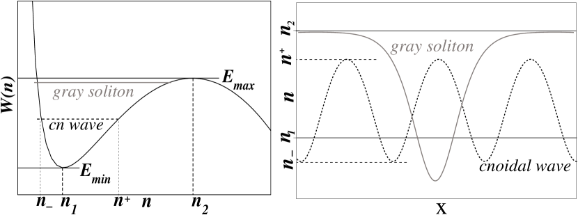
Figure 2: Plot of the function $W(n)$, here displayed for the low density regime ${\mathcal{E}}(n)=g\,n^{2}/2$, in the left panel. For given $\mu,j_{t}$ and $g$, a beam of uniform density has either a density $n_{1}$ (supersonic solution) or a density $n_{2}$ (subsonic solution). At a given classical energy $E$ (with $E_{min}<E<E_{max}$, to assure bounded density oscillations ), $n_{-}$ and $n^{+}$ are the minimum and maximum values of the cnoidal density oscillations, displayed in the right panel. Energy values $E$ close to (but lower than) $E_{max}$ correspond to gray solitons.

The left panel of Fig. 2 displays the potential $W(n)$ in the low-density regime where we have ${\mathcal{E}}(n)=gn^{2}/2$ with the effective interaction parameter $g\equiv 2\hbar\omega a_{s}n^{2}$. $W(n)$ has qualitatively the same form in the high-density regime as well where ${\mathcal{E}}$ is given by ${\mathcal{E}}(n)=2{\bf g}n^{3/2}/3$ with ${\bf g}\equiv 2\hbar\omega\sqrt{a_{s}}$ . For weak and moderate coupling constants $g$ (respectively ${\bf g}$), $W(n)$ exhibits a local minimum $E_{min}=W(n_{1})$ at a low density $n_{1}$ and a local maximum $E_{max}=W(n_{2})$ at a high density $n_{2}$. These extrema, at which the fictitious particle would be at rest forever, correspond to solutions of Eq. (19) with constant density. They represent plane waves of the form $\psi_{\nu}(x,t)=\sqrt{n_{\nu}}\exp(ik_{\nu}x-i\mu t/\hbar)$ ($\nu=1,2$) whose wave numbers $k_{\nu}$ are implicitly determined through the dispersion relation of the Gross-Pitaevskii equation , namely

$$\mu=\frac{m}{2}\frac{j_{t}^{2}}{n_{\nu}^{2}}+\epsilon(n_{\nu}),$$ (21)

as expressed in terms of the total current $j_{t}=\hbar k_{\nu}n_{\nu}/m$. The solutions $\psi_{1}$ and $\psi_{2}$ are termed “supersonic” and “subsonic”, respectively, since the beam velocity is larger than the speed of sound of the condensate for $\psi_{1}$ and smaller than the speed of sound for $\psi_{2}$ LebPav01PRA . The transport of particles at theses two solutions is dominated by the kinetic energy in the supersonic case, and by the interaction between the atoms in the subsonic case. We note that in the noninteracting limit, where $\epsilon(n)$ is independent of $n$, the subsonic density $n_{2}$ diverges and $W(n)$ has only one finite extremum at the density $n_{1}$.

Solutions of Eq. (17) with $E_{min}<E<E_{max}$ exhibit periodic density oscillations and correspond to a bounded motion of the fictitious classical particle. They are implicitly given through the integration of Eq. (19), i.e.

$$x-x_{0}=\int_{A(x_{0})}^{A(x)}\frac{\sqrt{2/m}\ \hbar\ dA}{E-m\,j_{t}^{2}/(2A^{2})-\mu A^{2}+{\mathcal{E}}(A^{2})},$$ (22)

where the amplitude $A(x_{0})$ at the position $x_{0}$ determines the initial value for the solution of the differential equation (17). For $\epsilon(n)=g\,n/2$ it was shown that the solutions of Eq. (22) can be expressed in terms of Jacobi-Elliptic functions RapWitKor06PRA .

For our purpose, a qualitative characterization of the free solutions of the Gross-Pitaevskii equation is sufficient: Small deviations from the constant density value $n_{1}$, e.g. small values of $E-W(n_{1})$ correspond to small sinusoidal density oscillations. Energy values close to (but lower than) the limiting classical energy value $E_{{max}}=W(n_{2})$ correspond to gray solitons. In the intermediate regime, between the limiting cases of small sinusoidal oscillations and gray solitons, the condensate density exhibits cnoidal oscillations. Energy values larger than $E_{\text{max}}$ lead to an infinite density at finite $x$ and cannot be interpreted as physically meaningful steady-state solutions. We also note that the flat-density solutions coincide, $n_{1}=n_{2}$, when the potential $W(n)$ exhibits a saddle point configuration. For the potential $W(n)$ displayed in Fig. 2, such a saddle point configuration would, e.g., be encountered by increasing $g$ while $\mu$ and $j_{t}$ are kept fixed. In the low density limit where $\epsilon(n)=2\hbar\omega_{\perp}a_{s}n$, the criterion for the existence of a saddle point configuration reads $8\mu^{3}=27mj^{2}g^{2}$; in the high density limit where $\epsilon(n)=2\hbar\omega_{\perp}\sqrt{a_{s}n}$, we find $\mu^{5}=5^{5}mj^{2}{{\bf g}}^{4}/2^{9}$. Beyond these limits no stationary solutions exists any more.

Finding stationary scattering states in presence of a finite scattering potential requires now to match two asymptotic density modes, each characterized by a separate integration constant $E$, in the upstream respectively downstream region. From general arguments on the dispersion relation of elementary excitations of the Gross-Pitaevskii equation follows that the physically meaningful boundary condition for the steady-state solutions of Eq. (17) demands a constant downstream density profile LebPav01PRA . The asymptotic downstream density should therefore correspond either to $n_{1}$ or $n_{2}$. In the present study, we intend to investigate the crossover from a noninteracting to a weakly or moderately interacting system. We therefore focus on the regime of rather small condensate densities, respectively weak atom-atom interactions ($na_{s}\ll 1$ and $\epsilon(n)=gn$); hence, the low-density downstream solution $n_{1}$ will be relevant in the following. The high-density solution $n_{2}$ exhibits qualitatively different features, such as solitonic transmission modes, and has been discussed in Ref. LebPavSin03PRA .

In analogy with the scattering problem in a non-interacting system we define a stationary scattering state as a solution of Eq. (9) of the form

$$\psi(x,t)=\psi(x)\exp(-i\mu t/\hbar),$$ (23)

satisfying, in the downstream region, outgoing boundary conditions of the form $\psi(x)=\sqrt{n_{1}}\exp(ikx)$, with $k>0$ given by $k_{1}$ as defined above. In order to determine the scattering states for a given barrier potential $V_{||}(x)$, which vanishes at $x\to\pm\infty$, and for given values for the total current flow $j_{t}$ and the chemical potential $\mu$, we integrate the equation of motion (17) from the downstream to the upstream region with the “asymptotic condition” $A=\sqrt{n_{1}}$ and $A^{\prime}=0$ in the downstream region. This allows us to compute the density profile in the whole waveguide, and by computing the phase via $S^{\prime}(x)=mj_{t}A^{2}(x)/\hbar$ we determine unambiguously the stationary scattering state $\psi(x)$. This procedure describes the scattering process in terms of a so-called fixed output problem, because the outgoing current $j_{t}$ in the downstream region enters as a parameter in the asymptotic boundary conditions that determine the scattering state GreKiv92PR ; KnaPapWhi91JSP .

There is only a small number of potential configurations, such as the square well or delta-peak barriers, for which the integration can be carried out analytically RapWitKor06PRA . For the general case, it is convenient to rewrite Eq. (17) in terms of Hamilton-like equations of motion

$$A^{\prime}=\frac{\partial{\mathcal{H}}}{\partial p} = \frac{m}{\hbar^{2}}p,$$

$$p^{\prime}=-\frac{\partial{\mathcal{H}}}{\partial A} = \left(\frac{mj_{t}^{2}}{A^{4}}-2[\mu-V_{\|}(x)-\epsilon(n)]\right)A,$$ (24)

where we introduced the canonical momentum $p\equiv(\hbar^{2}/m)A^{\prime}$. These equations of motions can be deduced from the classical Hamiltonian

$${\mathcal{H}}(A,p)=\frac{\hbar^{2}}{2m}p^{2}+\frac{mj_{t}^{2}}{2A^{2}}+[\mu-V_{\|}(x)]A^{2}-{\mathcal{E}}(A^{2}).$$ (25)

In the picture of the fictitious classical particle, $V_{||}(x)$ plays the role of a driving force which drives the particle away from the minimum of the classical potential $W(n)$. The classical energy, which is $E_{d}=W(n_{1})$ in the downstream region, is altered by the amount

$$\Delta E=\int_{-\infty}^{+\infty}V_{||}(x)A(x)A^{\prime}(x)dx,$$ (26)

which yields the new classical energy value $E_{u}=E_{d}+\Delta E$ for the upstream region. The asymptotic behavior of the scattering state is then fully determined by $E_{u}$ and $E_{d}$. The energy transfer $\Delta E$ is a measure for the amplitude of the density oscillations in the upstream region, i.e. increasing values of $\Delta E$ imply a larger backreflection.

Our purpose is now to determine the reflection and transmission coefficients, $T$ and $R$, associated with the stationary scattering states. These quantities are naturally given by $T=j_{t}/j_{i}$ and R=$j_{r}/j_{i}$, where $j_{i}$, $j_{t}$, and $j_{r}$ respectively denote the incident, transmitted, and reflected current of the condensate. The determination of $j_{i}$ and $j_{r}$, however, is a nontrivial task, since we can not simply decompose the upstream wave function into an incident and reflected plane wave component due to the nonlinearity of the Gross-Pitaevskii equation which does not permit the application of the superposition principle. We show now how the incident and reflected currents can nevertheless be defined and calculated in a meaningful way.

First, we briefly recall a method that has been suggested in Ref. LebPavSin03PRA and was successfully applied in Ref. PauO05PRA . It allows one to determine approximate values for $T$ and $R$ in the regime of small backreflections or small nonlinearities, by means of an approximate decomposition of the upstream density into an incident and reflected beam. We consider here the low density regime $a_{s}n\ll 1$, e.g. $\epsilon(n)=gn$. In the upstream region, $n(x)=A^{2}(x)$ obeys the equation [see Eq. (19)]

$$E_{u}=\frac{\hbar^{2}}{2m}\left(\frac{d\sqrt{n}}{dx}\right)^{2}+W(n)$$ (27)

with

$$W(n)=\frac{m~{}j^{2}}{2n}+\mu n-\frac{1}{2}\,gn^{2}.$$ (28)

We write the density in the form $n(x)=n_{1}+\delta n(x)$, where $\delta n(x)$ represents the density oscillations originating from back-reflections. Inserting this ansatz into Eq. (27) and introducing a new effective wave number

$$\kappa=k\sqrt{1-{1}/({2\,\xi^{2}k^{2}})}$$ (29)

(here, $\xi=\hbar/\sqrt{2mn_{1}g}$ is the condensate’s healing length in the downstream region) and the characteristic scale $\delta n_{1}={m}[E_{u}-W(n_{1})]/({\hbar^{2}\kappa^{2}})$ for density oscillations, we obtain

$$\left(\frac{d\delta n}{dx}\right)^{2}+4\kappa^{2}\delta n^{2}=8\kappa^{2}\delta n_{1}(n_{1}+\delta n)+\frac{4mg}{\hbar^{2}}\delta n^{3}$$ (30)

as an equation of motion for $\delta n(x)$.

Until now, no approximation has been made. In the regime of small back-reflections, where $|\delta n|/n_{1}\ll 1$ holds, or small interaction parameters $g$ (both limits are covered by the condition $|\delta n|/n_{1}\ll\kappa^{2}\xi^{2}$, see Ref. LebPavSin03PRA ), we neglect the cubic term in Eq. (30). Thus, the equation of motion (30) corresponds to the dynamics of a shifted harmonic oscillator, and its solution is given by

$$n(x)=n_{1}+\delta n_{1}+\sqrt{2n_{1}\delta n_{1}+(\delta n_{1})^{2}}\cos(2\kappa x+\theta),$$ (31)

where $\theta$ is an arbitrary phaser. The density profile (31) is equivalent to that of the two counterpropagating plane waves with wave vektor $\kappa$

$$\psi_{i}(x) = \sqrt{n_{1}+\frac{\delta n_{1}}{2}}~{}\exp(i\kappa x),$$

$$\psi_{r}(x) = \sqrt{\frac{\delta n_{1}}{2}}~{}\exp(-i\kappa x+i\theta),$$ (32)

yielding

$$n(x)=|\psi_{i}(x)+\psi_{r}(x)|^{2}.$$ (33)

Identifying $\psi_{i}(x)$ as an incident and $\psi_{r}(x)$ as a reflected wave component allows one to determine the transmission and reflection coefficients through

$$T=\left(1+\frac{\delta n_{1}}{2\,n_{1}}\right)^{-1},\quad R=\left(1+\frac{2n_{1}}{\delta n_{1}}\right)^{-1}.$$ (34)

The approximate nature of Eq. (34) becomes evident if we consider the conservation of currents. Computing the incident and reflected current components in the upstream region yields

$$j_{i}=\left(n_{1}+\frac{\delta n_{1}}{2}\right)\,\frac{\hbar\,\kappa}{m}\,,\quad j_{r}=\frac{\delta n_{1}}{2}\,\frac{\hbar\,\kappa}{m}\,,$$ (35)

whereas we find from the asymptotic downstream behavior of the wave function the transmitted current component $j_{t}=n_{1}\hbar k/m$. It is easy to see that the relation $j_{t}+j_{r}=j_{i}$ is exactly fulfilled only in the case of vanishing atom-atom interactions, i.e. $k=\kappa$. In the regime of weak interactions deviations from the current conservation are of the order ${\mathcal{O}}[(k\xi)^{-2}]$ and the approximate approach becomes inappropriate for strong interactions or large backreflections.

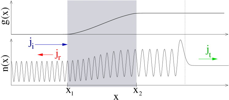
Figure 3: (color online) Adiabatic transition of the interaction parameter $g$ for a proper definition of transmission coefficients: The upper part of the figure displays the adiabatic variation of the position-dependent parameter $g(x)$ from $g=0$ up to a maximal value $g$. The gray-shaded transition region between $x_{1}$ and $x_{2}$ in which $g$ varies with position is assumed to be much larger than the typical periodicity of the condensate density oscillations. The lower part shows the density of a stationary scattering state in presence of a potential barrier, which is constant in the downstream region and displays oscillations in the upstream region (the position of the barrier potential is marked by the vertical line). The nonlinear cnoidal oscillation of $n$ between the barrier and $x_{2}$ is adiabatically conveyed, in the transition region between $x_{1}$ and $x_{2}$, into a sinusoidal oscillation in the interaction-free domain on the left-hand side of $x_{1}$. There, the wave function can be linearly decomposed into an incident and a reflected component.

In order to overcome this problem, we consider a waveguide configuration in which the interaction strength $g$ tends to zero for $x\to-\infty$ and reaches a finite constant value in the region where the barrier potential is located (see Fig. 3). We furthermore assume that the typical length scale on which $g$ varies is much larger than the periodicity of the density oscillations. Such a variation of $g$ can e.g. be achieved by decreasing the transverse confinement frequency $\omega$ of the waveguide or by tuning the scattering length $a_{s}$ via a Feshbach resonance.

Using once more the analogy with the dynamics of a classical particle, we introduce the effective “pseudo action”

$${\mathcal{J}}=\oint p\,dA=\frac{\hbar^{2}}{m}\int_{x_{0}}^{x_{0}+\Delta x}[A^{\prime}(x)]^{2}dx$$ (36)

that is integrated over one spatial period $\Delta x$ of the upstream density oscillation (which would be given by $\Delta x=\pi/k$ in the absence of the interaction). By use of Eq. (19) the pseudo action can also be written in the form

$${\mathcal{J}}=\hbar\,\sqrt{\frac{2}{m}}\,\int_{{n_{-}}}^{{n_{+}}}\sqrt{[E_{u}-W(n)]/{n}\,}\,dn,$$ (37)

where ${n_{-}}$, (${n_{+}}$) is the minimal (maximal) density value of the oscillating upstream density. It is determined via the relation $W(n_{\pm})=E_{u}$. Due to the theorem of adiabatic invariants, ${\mathcal{J}}$ remains approximately constant along the waveguide as long as $g$ is sufficiently slowly varied. It can, under this condition, therefore be evaluated at any position $x$, in particular also in the far-upstream region at $x<x_{1}$ where we have $g=0$. There we can decompose the wave function in an incident and reflected part as

$$\psi(x)=(\alpha\text{e}^{i(kx+\varphi)}+\beta\text{e}^{-ikx})\text{e}^{i\phi}$$ (38)

with $k=\sqrt{2m\mu}/\hbar$, where the amplitudes $\alpha,\beta$ and the phases $\varphi,\phi$ are real. The wave function’s amplitude reads

$$A(x)=\sqrt{\alpha^{2}+\beta^{2}+2\alpha\beta\cos(2kx+\varphi)},$$ (39)

and the canonical momentum $p$ is given by

$$p(x)=\frac{\hbar^{2}}{m}A^{\prime}(x)=\frac{2\alpha\beta k\sin(2kx+\varphi)}{\sqrt{\alpha^{2}+\beta^{2}+2\alpha\beta\cos(2kx+\varphi)}}.$$ (40)

By use of $dA=A^{\prime}dx$, we evaluate Eq. (36) as

$${\mathcal{J}}=\oint p\,dA,=2\beta^{2}\,\hbar^{2}k\pi/m.$$ (41)

Using the fact that the incident and reflected currents read $j_{i}=\hbar k\alpha^{2}/m$ and $j_{r}=\hbar k\beta^{2}/m$ in the far-upstream region, we can obtain the reflection and transmission coefficients via

$$R = \frac{j_{r}}{j_{i}}=\frac{\beta^{2}}{\alpha^{2}}=\left(1+\frac{2\pi\hbar j_{t}}{{\mathcal{J}}}\right),$$

$$T = 1-R=1-\frac{\beta^{2}}{\alpha^{2}}=\left(1+\frac{{\mathcal{J}}}{2\pi\hbar j_{t}}\right)^{-1}.$$ (42)

Eq. (II.2) unambiguously assigns a reflection and a transmission value to each scattering state that is a solution of the nonlinear wave equation (9). This definition represents a natural extension of the concept of transmission for nonlinear scattering problems.

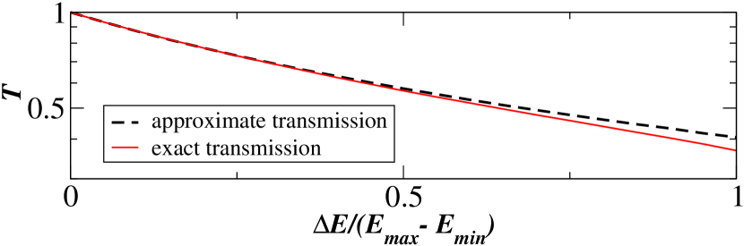
Figure 4: (color online) Comparison between the approximate and exact transmission values, calculated with Eqs. (II.2) and (34) respectively, for a moderately interacting condensate that propagates through a potential barrier, with the dimensionless parameters $\mu=3$, $g=1/2$, $j_{t}=1$, and with variable barrier height. The transmission is plotted as a function of the classical energy transfer $\Delta E$, which is a measure for the back-reflection in the upstream region. For increasing back-reflections, the approximate result (34) overestimates the “true” value of the transmission coefficient given by Eq. (II.2).

For the practical computation of the transmission value associated with a given scattering state, it is sufficient to evaluate the integral (37) numerically in the near-upstream region (i.e. for $x\simeq x_{2}$ in Fig. 3) where the extremal densities $n_{\pm}$ can be found by solving $W(n_{\pm})=E_{u}$. This means that the adiabatic variation of $g$ does not need to be included at all in the calculation; it is sufficient to take into account a short spatial domain in the upstream region within which the condensate exhibits a couple of density oscillations. Computing the transmission by use of Eq. (II.2) circumvents the approximate character of the relation (34) and is therefore also valid in the regime of strong atom-atom interactions as well as for large back-reflections. In Fig. 4 we compare the approximate with the “exact” expression for the transmission, determined by Eqs. (34) and (II.2) respectively, for a condensate with a moderate nonlinearity that encounters a potential barrier in the guide. For small large back-reflections both results coincide, whereas for large back-reflections the approximate formula (34) systematically overestimates the transmission.

II.3 Time-dependent transport processes

So far, we restricted our considerations to stationary scattering solutions of the time-independent Gross-Pitaevskii equation. A severe problem is the fact that the mere existence of a stationary scattering state does not imply that this state is dynamically stable and can be populated in a time-dependent scattering process. This is not only true for the propagation of a finite wave packet (which obviously cannot be evolved by an expansion in terms of stationary solutions of the Gross-Pitaevskii equation , due to the absence of superposition principle), but also concerns the limiting case of a quasi-stationary flow that is generated by an adiabatic injection of the condensate into the waveguide. This affects, as we shall discuss later on, the resonant transport of a condensate through a double barrier potential, where the dynamical stability properties of the scattering states become crucial for their population.

In view of this complication we now describe a method based on the time-dependent Gross-Pitaevskii equation , which allows us to simulate a realistic propagation process. This equation is integrated in presence of an inhomogeneous source term, located at a position $x=x_{0}$ in the upstream region and emitting monochromatic matter waves. The source term simulates the coupling of the waveguide to a large reservoir of a Bose-condensed matter at a given chemical potential $\mu$, from which matter waves are injected into the waveguide (see Fig. 5). The effective nonlinear wave equation that governs the time evolution of the condensate wave function $\psi(x,t)$ is therefore given by

$$i\hbar\frac{\partial\psi(x,t)}{\partial t} = \left[-\frac{\hbar^{2}}{2m}\frac{\partial^{2}}{\partial x^{2}}+V_{||}(x)+g|\psi(x,t)|^{2}\right]\psi(x,t),$$ (43)

$$+S(t)~{}\delta(x-x_{0})~{}\exp{(-i\mu t/\hbar)},\;$$

where the time-dependent coupling strength between the waveguide and the reservoir is contained within the source amplitude $S(t)$. The interaction parameter $g$ need not be constant, but may be considered to position-dependent as well, in order, e.g., to simulate the adiabatic transition from a noninteracting to an interacting guide as depicted in Fig. 3. In this work, we restrict ourselves to the case where $g$ is constant in the vicinity of the finite-range scattering potential.

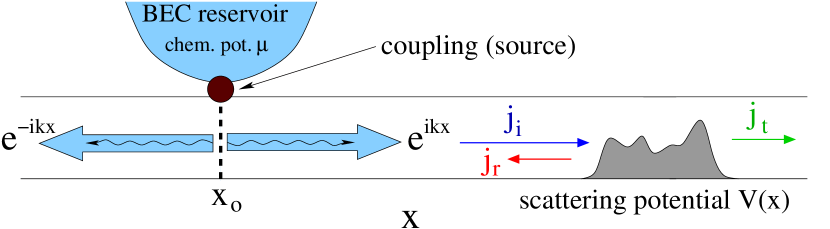
Figure 5: (color online) A reservoir of Bose-condensed matter with a given chemical potential $\mu$ is locally coupled at the position $x_{0}$ to a waveguide with a scattering potential. The reservoir emits a plane matter wave in both directions into the guide. Hence, a coherent beam, with current $j_{i}$, propagates towards the barriers of the potential where the condensate is partially reflected, with the current $j_{r}$, and partially transmitted, with the current $j_{t}$.

Before studying time-dependent scattering processes in a waveguide with a finite scattering potential, it is instructive to consider first stationary solutions of Eq. (43) for the particular case of a homogeneous waveguide, i.e. $V_{||}(x)\equiv 0$, and a constant source amplitude $S(t)\equiv S_{0}$. In this case, there exist plane wave solutions $\psi(x,t)=\psi(x)e^{-i\mu t}$ with constant density $n=|\psi(x,t)|^{2}$. To demonstrate this, we switch to the Fourier space by introducing the Fourier transformed wave function $\tilde{\psi}(q,t)=\int\exp(iqx)\psi(x,t)dq$. Then, Eq. (43) takes the form

$$\left({i}{\hbar}\frac{\partial}{\partial t}-\frac{\hbar^{2}\,q^{2}}{2m}-gn\right)\tilde{\psi}(q,t)=S_{0}\,e^{-iqx_{0}}\,e^{-i\mu t/\hbar}\;.$$ (44)

This equation admits solutions of the form

$$\tilde{\psi}(q,t)=\frac{2mS_{0}\,e^{-iqx_{0}}}{\hbar^{2}k^{2}-\hbar^{2}q^{2}}\,e^{-i\mu t/\hbar}\;.$$ (45)

Here, we introduced the wave vector $k$ via the relation $\hbar^{2}k^{2}=2m(\mu-gn)$. By transforming back to the position space, we find solutions where the source term emits in both directions the monochromatic wave

$$\psi(x,t)=\frac{S_{0}m}{ik\hbar^{2}}\;e^{ik|x-x_{0}|}\;e^{-i\mu t/\hbar},$$ (46)

with the wave number $k$ being self-consistently defined by

$$k^{2}=\frac{1}{\hbar^{2}}\left[{2m\left(\mu-g\frac{|S_{0}|^{2}m^{2}}{\hbar^{4}k^{2}}\right)}\right].$$ (47)

The density that is associated with the wave function (46) reads

$$n=\frac{|S_{0}^{2}|m^{2}}{(\hbar^{4}k^{2})}=\frac{|S_{0}|^{2}m}{2\hbar^{2}(\mu-gn)}.$$ (48)

Evaluating the quantum mechanical current operator shows that the source emits the current

$$j_{i}=\pm\frac{|S_{0}|^{2}m}{(\hbar^{3}k)}\ \overset{(\ref{390})}{=}\ \pm\frac{1}{\hbar}|S_{0}|\sqrt{n},$$ (49)

with “ $+$ “ for $x>x_{0}$ and “$-$ “ for $x<x_{0}$. Inserting Eq. (49) into Eq. (48) immediately yields the plane-wave dispersion relation $\mu=mj_{i}^{2}/(2n^{2})+gn$.

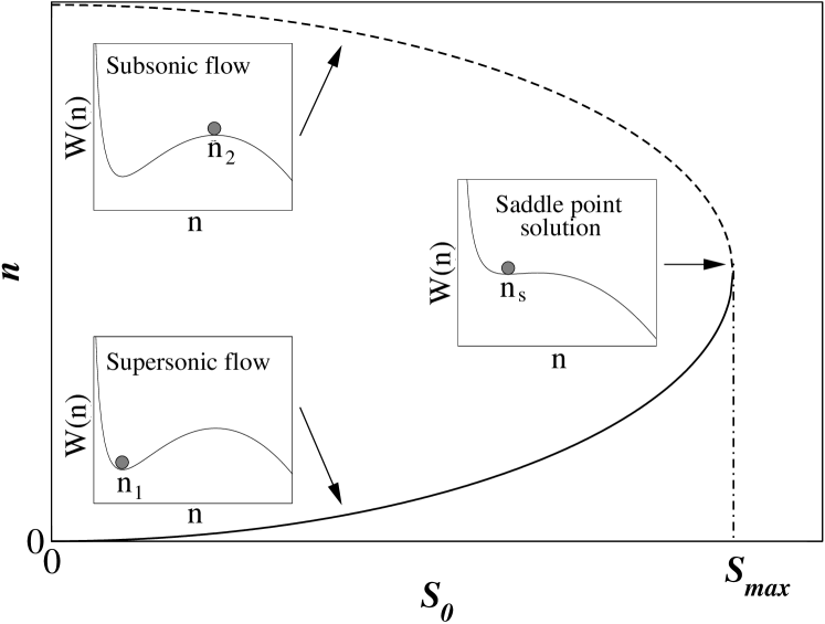
Figure 6: Illustration of the relation (50) between the source amplitude $S_{0}$ and the densities $n_{1,2}$ of a homogeneous flow. The lower branch corresponds to the supersonic solutions with density $n_{1}$ and the upper branch to the subsonic solutions with density $n_{2}$. The insets illustrate the configuration of the classical potential $W(n)$ for the different types of solutions.

As already discussed in Sec. II.2 (see Eq. (21)) this equation admits two flat-density solutions, $n=n_{1}$ and $n=n_{2}$, corresponding to a supersonic and a subsonic propagation of the condensate, respectively. Rewriting Eq. (48) in the form

$$n_{1,2}=\frac{1}{2g}\left(\mu\mp\sqrt{\mu^{2}-2gm|S_{0}|^{2}/\hbar^{2}}\right)$$ (50)

allows one to compute the two densities $n_{1,2}$ that are possible for a given value of the source amplitude $S_{0}$. This relation is illustrated in Fig. 6: the lower branch contains the supersonic solutions and the upper branch the subsonic solutions. The value $S_{max}=\hbar\mu/\sqrt{2gm}$ corresponds to the saddle point configuration of the classical potential $W(n)$; for source amplitudes larger than this threshold, no stationary solutions of Eq. (43) are possible. In the limit of noninteracting particles, $g=0$, only the supersonic branch survives (because the speed of sound is zero) and Eq. (50) takes the simple form $n=|S_{0}|^{2}m/(2\hbar^{2}\mu)$.

Now we study the time evolution of $\psi(x,t)$ in presence of a variable source amplitude $S(t)$. Here, the scenario of an initially empty waveguide that is gradually filled with matter waves is of peculiar interest as this corresponds to the experimentally realistic situation where the condensate is initially confined in a microtrap (playing the role of the reservoir) and then smoothly released to propagate into the waveguide. To simulate such a process, we propagate $\psi(x,t)$ by numerically integrating the wave equation (43) in presence of an adiabatic increase of the source amplitude $S(t)$ from $S(t=0)=0$ up to a given maximal value $S_{0}$, with the initial condition $\psi(x,t=0)\equiv 0$. The amplitude $S(t)$ is increased adiabatically in order to ensure that, at any instant during the propagation, the wave function in the guide remains as close as possible to a stationary scattering state of the form $\psi(x)\exp(-i\mu t/\hbar)$. Quantitatively this means that the typical time scale $\Delta T$ on which the amplitude $S(t)$ increases is much larger than the characteristic time scale $\tau\equiv\hbar/\mu$ that is associated with the chemical potential $\mu$ of the source: $\Delta T\gg\tau$. As we are studying an infinitely extended scattering problem, we have to impose absorbing boundary conditions in order to avoid artificial back-reflection at the boundaries of the numerical grid. Details on these absorbing boundaries, which are taken from Ref. Shibata and adapted to account also for a finite nonlinearity, as well as on the numerical integration procedure are given in Appendix B.

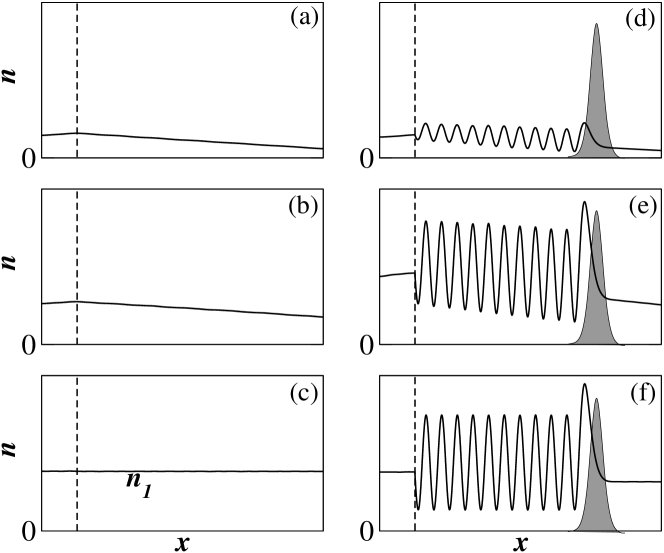
Figure 7: Time evolution of the condensate density during the adiabatic increase of the source amplitude (the source is located at the vertical dashed lines). The panels (a-c) show three snapshots of the condensate in a waveguide without scattering potential: at (a) $t=0.1\,\Delta T$, (b) $t=\Delta T$, and (c) $t=10\,\Delta T$. The bottom part of the figure shows the real and imaginary part of the wave function whose density is displayed in panel (b). The panels (d-f) illustrate the scattering of the matter waves at a repulsive barrier potential (gray-shaded region). Panel (f) clearly shows that a stationary scattering state is populated in the long-time limit $t\gg\Delta T$.

In a first step we discuss the filling of the waveguide in absence of a scattering potential, i.e. for $V_{||}(x)\equiv 0$. Fig. 7(a-c) displays the time-evolution of the wave function $\psi(x,t)$ by a series of snapshots showing the density at different times. For the sake of definiteness we chose $S(t)=S_{0}[1-\exp(-t/\Delta T)]\$, which provides a smooth evolution towards the desired final value $S(t\to\infty)=S_{0}$. We find that for propagation times $t\gg\Delta T$ the calculation converges towards the flat density (Fig. 7c) that corresponds to the stationary plane wave (46) at the source amplitude $S=S_{0}$. The bottom part of Fig. 7 shows the real and imaginary parts of the wavefunction $\psi$ at the time $t=\Delta T$ during the filling process. These panels clearly illustrates that the source emits a plane-wave like solution of the form $A(x,t)\exp[-i\mu t+ik(x,t)x]$ where $A(x,t)$ and $k(x,t)$ vary slowly with position and time.

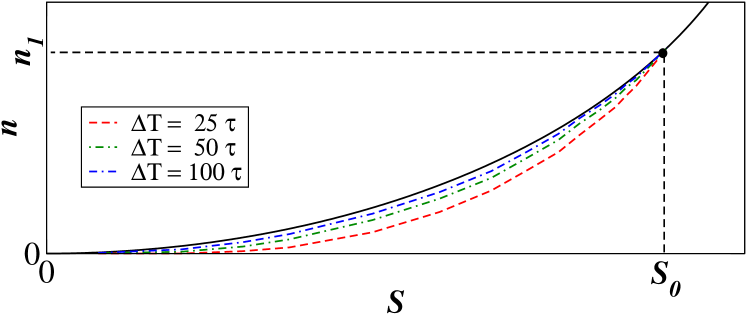
Figure 8: (color online) Evolution of the condensate density as a function of the source amplitude $S$ for three different values of the time scale $\Delta T$ in which $S$ is ramped to its maximal value $S_{0}$ (dashed and dashed-dotted curves). For an increasing ratio $\Delta T/\tau$ with $\tau\equiv\hbar/\mu$, the curves converge towards the supersonic branch of Eq. (50) (solid line). For $S\to S_{0}$ the supersonic scattering state with constant density $n=n_{1}$ is reached.

It is instructive to display the evolution of the condensate density as a function of the time-dependent source amplitude $S$. Fig. 8 shows this evolution for different values of $\Delta T$ (dashed lines). We notice that these curves approach the lower branch of the relation (50) (solid line in Fig. 8, see also Fig. 6) if we reach the limit $\Delta T\gg\tau$. We therefore deduce that the adiabatic filling of an initially condensate-free waveguide can only populate stationary solutions that correspond to a supersonic flow; hence, the final condensate density is given by $n=n_{1}$ as defined by Eq. (50). In analogy to the fixed output problem discussed in Sec. II.2, the implementation of the source term therefore allows one to investigate the transport of the condensate in terms of a so-called fixed input problem, where the incident current $j_{i}$ that is emitted into the guide parametrizes the process. The fixed input approach is much closer to experimental situations because the current that is injected into the guide is typically under much better control than the total transmitted current $j_{t}$.

In a second step, we consider a scattering process in presence of a barrier potential $V_{||}(x)$. Due to the partial backscattering of the condensate at the barrier, the dynamics becomes more complex as compared to the potential-free case. Nevertheless, for weak or moderate nonlinearities the wave function $\psi(x,t)$ is found to converge towards a stationary scattering state $\psi(x)\exp(-i\mu t/\hbar)$ during the adiabatic increase of the source amplitude towards its final value $S_{0}$, as illustrated in Fig. 7(d - f). During the gradual filling of the guide, the condensate is partially reflected at the barrier, which leads to the oscillating density pattern between the barrier and the position of the source in the upstream region. On the right-hand side of the barrier, in the downstream region, the density is flat in the long-time limit $t\gg\Delta T$, which reflects the fact that the wave function $\psi(x)$ is given there by an outgoing plane wave of the form $\psi(x)=A\exp(ikx)$. We checked that the state $\psi(x)$ that is reached at the end of the propagation fulfills the stationary Gross-Pitaevskii equation, i.e., the wave function’s amplitude $A(x)={|\psi(x)|}$ is a solution of Eq. (17).

Once we populate a stationary state, we have another straightforward access to the transmission coefficient $T$ in the nonlinear scattering problem: $T$ is given by the ratio of the transmitted current $j_{t}$, evaluated through the current operator in the downstream region, to the current that would propagate through the waveguide in absence of the barrier potential, which is the current $j_{i}$ that is directly emitted from the source. This approach provides another natural extension of the definition of transmission coefficients to nonlinear wave equations. Hence, the numerical method introduced in this section allows not only to calculate scattering states that are dynamically stable and can be populated in a realistic propagation process Bemerkung1 , but provides also a straightforward access to transmission coefficients for a fixed input problem.

We point out that in the nonlinear case, convergence towards a stationary scattering state is not always guaranteed. Indeed, studying the transport of condensates through a waveguide with an extended disorder region by means of the method described in this section revealed that, beyond a critical interaction strength respectively a critical length of the disorder region, the transport process generally remains time-dependent and stationary states are not populated PauO05PRA .

II.4 Transport through a quantum point contact

As a first and simple example we study the transport of a Bose-Einstein condensate through a quantum point contact. We consider a waveguide with a constriction given by a single repulsive Gaussian barrier potential $V_{||}(x)=V_{0}\exp(-x^{2}/\sigma^{2})$ which can be experimentally implemented by focusing a blue detuned laser beam in its transverse ground mode onto the waveguide Engels . For the sake of definiteness we consider in the following a condensate of ⁸⁷Rb atoms ($m=1.45\times 10^{-25}kg$, $a_{s}=5.77$ nm) flowing through a waveguide with transverse trapping frequency $\omega=2\pi\times 10^{3}$ s^-1 that corresponds to a harmonic oscillator length $a_{\perp}=0.34$ $\mu$m. It is convenient to measure energies in units of $\hbar\omega$, lengths in units of $a_{\perp}$ and particle currents in units of $\omega$. In these units the interaction parameter reads $g=0.034\hbar\omega a_{\perp}$. For the longitudinal extension of the barrier we assume $\sigma=2a_{\perp}\simeq 0.7\mu m$ (which would be at the limit of experimental realizability) and its height is chosen as $V_{0}=3\,\hbar\omega$.

In a first step, we investigate the transport process in terms of a fixed output problem: We calculate scattering states by integrating the stationary Gross-Pitaevskii equation,

$$\mu\psi(x)=\left[-\frac{\hbar^{2}}{2m}\frac{\partial^{2}}{\partial x^{2}}+V_{0}e^{-x^{2}/\sigma^{2}}+g|\psi(x)|^{2}\right]\psi(x),$$ (51)

for given values of the chemical potential $\mu$ and the transmitted current $j_{t}$ from the downstream to the upstream region (where a supersonic density $n(x\to\infty)=n_{1}$ is assumed in the downstream region). Eq. (II.2) allows us to compute the corresponding transmission coefficient from which we can deduce the incident current via $j_{i}=j_{t}/T$. Varying the transmitted current allows us to compute the $j_{t}-j_{i}$ current characteristics which is displayed for $\mu=3\hbar\omega$ in the inset of Fig. 9. For noninteracting particles ($g=0$) the $j_{t}-j_{i}$ characteristics is linear, because the transmission coefficient $T$ does not depend on the particle current, whereas for non-vanishing interaction parameters the $j_{t}-j_{i}$ characteristics shows a nonlinear behavior and displays increasing deviations from the linear case with increasing particle currents. This means that the presence of repulsive interactions suppresses the transmission through the quantum point contact with growing current.

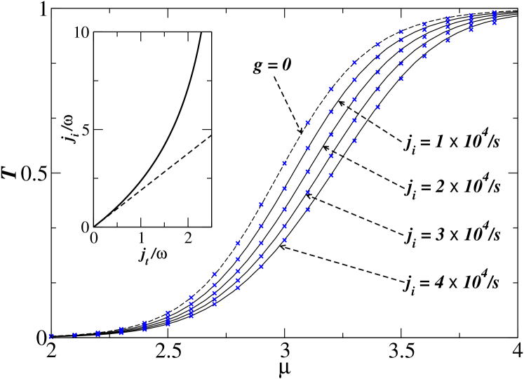
Figure 9: (color online) Transmission spectrum of the condensate flow through a quantum point contact for different values of the incident current $j_{i}$ ($\mu$ in units of $\hbar\omega$). The solid lines are found by evaluating the stationary Gross-Pitaevskii equation, the values denoted by crosses are obtained by integrating the time-dependent Gross-Pitaevskii equation in presence of the source term (the dashed line displays the result for a noninteracting condensate). The inset shows the $j_{t}-j_{i}$ current characteristics for a condensate flow without interactions ($g=0$, dashed line) and in presence of interactions ($g=0.034\hbar\omega$, solid line), at $\mu=3\hbar\omega$.

It is now easy to switch from the fixed output to the fixed input problem where the incident current $j_{i}$ is kept constant. To this end, we basically have to invert the $j_{t}-j_{i}$ characteristics, in order to determine the total current $j_{t}$ and the corresponding transmission coefficient $T$ that result from a given incident current $j_{i}$. This can be done in a unique way in the present case, since the $j_{t}-j_{i}$ characteristics is monotonous and therefore allows one to unambiguously assign to each value of $j_{t}$ a unique incident current $j_{i}$. Computing the current characteristics for different values of $\mu$ allows one then to obtain the transmission spectrum, i.e. the transmission coefficient $T$ as a function of the chemical potential $\mu$ at a fixed incident current $j_{i}$. Transmission spectra of the point contact for different incident currents are displayed in Fig. 9. Qualitatively, we find that in presence of repulsive interactions the spectra resemble strongly the spectrum for a single particle: for chemical potentials considerably smaller than $V_{0}$ the transmission tends to zero, whereas for $\mu$ much larger than $V_{0}$ we reach a regime of perfect transmission. In the intermediate regime, we clearly see that increasing particle currents $j_{i}$ yield a moderate suppression of the condensate flow through the point contact. This is attributed to the fact that the presence of the repulsive interaction leads, at fixed $\mu$, to a reduction of the available kinetic energy, which in turn reduces the probability for the atoms to penetrate the barrier.

So far, the computation of the transmission spectra was based on the stationary Gross-Pitaevskii equation. As a complementary access, we apply the method based on integrating the time-dependent Gross-Pitaevskii equation with source term. For each value of $\mu$, the wave function was propagated according to Eq. (44) in the presence of an adiabatic increase of the source amplitude $S$ up to the maximum value $S_{0}$ that corresponds to a given incident current $j_{i}$. For the considered range of incident currents $j_{i}$ we find stationary scattering states at the end of the propagation. As shown in Fig. 9, the results for the transmission obtained from the time-dependent integration (marked by blue crosses) coincide with the result based on evaluating the stationary Gross-Pitaevskii equation. Hence we can conclude that a gradual filling of the guide populates precisely those scattering states that are eigenmodes of the stationary problem, and that these stationary states are dynamically stable.

III Transport through a double barrier potential

Now we study the particularly interesting propagation process of a Bose-Einstein condensate through a symmetric repulsive double barrier potential which can be seen as a Fabry-Perot interferometer for matter waves. This setup was first discussed by Carusotto and La Rocca CarLar99PRL ; Car01PRA who proposed to use a combination of optical lattices for the realization of this bosonic quantum dot. In the context of atom chips, a double barrier potential could also be implemented by suitable geometries of microfabricated wires on a multilayer chip geometry Bem1 . Another straightforward implementation relies on two blue-detuned parallel laser beams, crossing transversely the waveguide. Assuming the laser beams to be in the lowest transverse mode, this setup creates a potential geometry with two Gaussian shaped barriers. For the sake of definiteness, we consider this latter case and assume a double barrier given by

$$V_{db}(x)=V_{0}\left[e^{-(x+L/2)^{2}/\sigma^{2}}+e^{-(x-L/2)^{2}/\sigma^{2}}\right].$$ (52)

Here, $\sigma$ is the width of one barrier and $L$ is the distance between the barriers.

For a flow of noninteracting particles it is well known that the transmission spectrum of a symmetric double barrier potential exhibits Breit-Wigner resonances Ferry which are related to resonant transport states. In our context, these resonant states can be defined as stationary scattering states of the condensate (see Eq. (23) ) that exhibit perfect transmission. In the following, we investigate to which extent resonant transport through such a double barrier potential can be achieved for an interacting condensate, and how interactions modify the transmission spectrum.

III.1 Resonant transmission spectra

We now compute transmission spectra for the double barrier potential (52) by applying the same methods that have been employed to find the spectra of the quantum point contact in Sec. II.4, using again the same units that were already introduced there. In the following, we consider a condensate with effective interaction strength $g$ (which will be varied to investigate the effect of an increasing nonlinearity), a waveguide with transverse trapping frequency $\omega=2\pi\times 10^{3}s^{-1}$, and a double barrier potential (52) with the parameters $V_{0}=1.1\,\hbar\omega$, $\sigma=a_{\perp}$, and $L=4.25a_{\perp}$. We study the transport of the condensate in terms of a fixed input problem, with incident current $j_{i}=1.0\,\omega$. The influence of the atom-atom interaction on the transmission spectrum is exemplarily investigated in the vicinity of the energetically lowest resonance which has one density maximum in between the two barriers (see inset in Fig. 10). In Ref. PauRicSch05PRL we showed that qualitatively similar results are also found for higher resonances.

First we compute transmission spectra by use of the integration method based on the stationary Gross-Piatevskii equation, respectively Eq. (17): The spectrum is, as in Sec. II.4, determined by calculating stationary scattering states for given $j_{t}$ and $\mu$, and the incident current of the scattering states is computed via Eq. (II.2). Finding the value of $j_{t}$ that results from a given $j_{i}$ is an optimization problem that can be solved systematically by analyzing the $j_{t}-j_{i}$ current characteristics. In the linear case, $g=0$, we obtain a Breit-Wigner resonance at $\mu=0.389\hbar\omega$ corresponding to the energetically lowest resonance state (Fig. 10).

Now we consider the case of a weak atom-atom interaction, $g=0.002\hbar\omega a_{\perp}$. As the most striking result, we find, close to the resonance, a multivalued transmission spectrum where two further solutions appear for $0.419<\mu/(\hbar\omega)<0.472$. These solutions join together to form a resonance peak that is asymmetrically distorted towards higher values of the chemical potential Bem333 . The resonant state, which is found at $\mu=0.472\hbar\omega$, coexists with a low-transmission state, as depicted in the central panel of Fig. 10. The asymmetric distortion becomes even more pronounced for an increasing interaction strength. This is shown in the bottom panel of Fig. 10 where we dipslay the spectrum in the vicinity of the first resonance for $g=0.01\hbar\omega_{\perp}$.

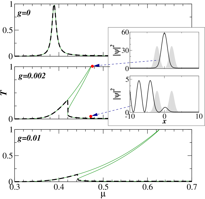
Figure 10: (color online) Transmission spectra of the double barrier potential at $g=0$ (upper panel), $g=0.002$ $\hbar\omega a_{\perp}$ (middle panel), and $g=0.01$ $\hbar\omega a_{\perp}$ (lower panel). The (green) solid lines show the transmissions of all scattering states, calculated by the “stationary” method based on Eq. (17), that exist at the incident current $j_{i}=1.0\,\omega$ of the matter-wave beam. The dashed lines display the spectra obtained from the time-dependent integration approach. The inset shows the longitudinal atom densities (in units of $a_{\perp}^{-1}$) of the first resonant state and the coexisting low-transmission state for $g=0.002$ $\hbar\omega a_{\perp}$ (the position $x$ is given in units of $a_{\perp}$). The gray-shaded curves indicate the positions of the two barriers. The (red) dots (marked by the arrows) designate the positions of the resonant state and the low-transmission state in the transmission spectrum.

It is instructive to trace the evolution of the $j_{t}-j_{i}$ characteristics in the vicinity of the onset of the multivalued subzone in the spectrum. In contrast to the monotonously increasing current characteristics that we found for the quantum point contact (Fig. 9), the characteristics of the double barrier potential shows a more complex behavior, where it is not always possible to unambiguously attribute to each incident current $j_{i}$ one single transmitted current $j_{t}$. Fig. 11 shows that for values of $\mu$ below the critical chemical potential from which on three branches coexist, the current characteristics intersects only once the horizontal line that represents the fixed incident current $j_{i}=1.0\,\omega$. Above this critical value of $\mu$ three intersection points are found, corresponding to the three coexisting scattering states.

Our findings are characteristic for a bistability phenomenon, similar to processes in nonlinear optics BoydBook and in the electronic transport through quantum wells Goldman87 ; Azbel99 . It is crucial to know which branches of the transmission spectrum are actually populated in a realistic experimental situation in order to decide if resonant transport is possible in presence of a finite interaction strength. To this end, we recalculate the transmission spectrum with the time-dependent integration approach, which simulates, at given value of $\mu$, the adiabatic release of the condensate from the reservoir into the waveguide. As explained in Sec. II.4, this method provides another straightforward access to the transmission values, and stationary states that are selected by this method automatically satisfy the criterion that they are dynamically stable and can be populated in a realistic propagation process.

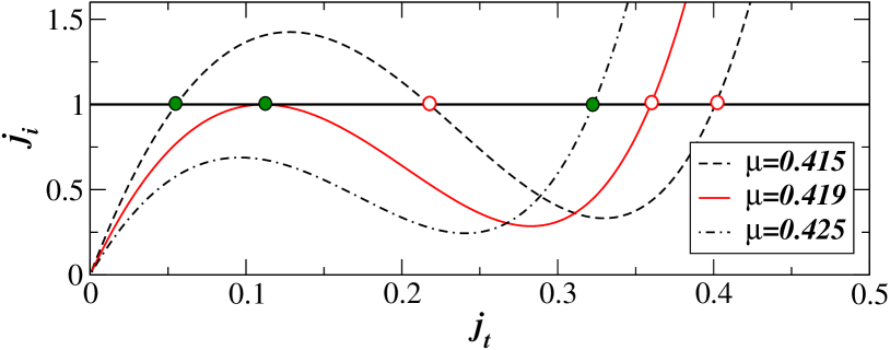
Figure 11: (color online) Current characteristics for the double barrier potential in the vicinity of the onset of the multivalued subzone of the spectrum (for $g=0.002$ $\hbar\omega a_{\perp}$). Below the critical $\mu=0.419\hbar\omega$, the $j_{i}-j_{t}$ characteristics (dashed-dotted line) intersects only once the horizontal line indicating the fixed incident current $j_{i}=1.0\,\omega$. Above this critical value, three intersection points are found (dashed line). At $\mu=0.419\hbar\omega$, the current characteristics (solid line) exhibits a tangent to the horizontal line. The intersection points marked with filled (green) points correspond to scattering states that are populated during a time-dependent propagation process.

The dashed lines in Fig. 10 show the result of this calculation. While a perfect agreement with the method based on the stationary Gross-Pitaevskii equation is found for $g=0$, the time-dependent approach reproduces, for $g\neq 0$, only the lowest branches of the spectra in the multivalued region. This apparently implies that the asymmetrically distorted peak structure is essentially inaccessible in the propagation process that is considered here. We therefore conclude that resonant transport, which would necessarily require the population of such a distorted peak, will generally be suppressed in presence of finite interactions, and only the low branches of the spectrum which have rather low transmission will be populated. Qualitatively, this behavior of the nonlinear system can be understood by comparing the “internal” interaction energy (evaluated within the internal region of the double barrier)

$$E_{\text{int}}=g\int_{-L/2}^{+L/2}|\psi(x)|^{2}\,dx$$ (53)

of the resonant with the one of the coexisting low-transmission state. The system can minimize $E_{\text{int}}$ by realizing a state with a low particle density in between the barriers. As displayed in the inset of Fig. 10, this favors the low-transmission state.

To conclude this section, we remark that a temporary enhancement of the transmission of matter waves near the resonance can be achieved by a variation of the external potential during the propagation process. In Ref. PauRicSch05PRL we devised a temporal modulation scheme where the potential is shifted with time according to $V(x)\to V(x,t)\equiv V(x)-V_{0}(t)$. Specifically, such a modulation can be induced by illuminating the scattering region with a red-detuned laser pulse, where $V_{0}(t)>0$ would be determined by the detuning and the intensity of the laser. In the case of an adiabatic modulation of $V$, the wave function $\psi(x,t)$ remains, at each time $t$, close to the instantaneous scattering state that is associated with the external potential $V(x,t)$ — or, equivalently formulated, close to the scattering state for the potential $V(x)$ at the shifted chemical potential $\mu+V_{0}(t)$. As soon as $\mu+V_{0}(t)$ is raised above the critical chemical potential from which on the transmission spectrum becomes multivalued, the wave function follows continuously the upper branch of the resonance and evolves into a near-resonant scattering state with high transmission. This state turns out to be dynamical unstable, and the wave function decays after a typical lifetime of the order of several milliseconds towards a low-transmission state PauRicSch05PRL .

III.2 Transmission in terms of quasi-bound states

In this subsection, we present analytical and numerical evidence that the distortion of the resonance peak arises indeed due to the nonlinearity-induced level shift of the self-consistent quasi-bound state within the atomic quantum dot. We describe, for this purpose, our system in a similar way as in the well-known scattering matrix approach MahWei , namely by a discrete “bound” (or quasi-bound) state within the quantum dot that is weakly coupled to two symmetric continua of unbound “lead” states in the up- and downstream regions of the waveguide. In contrast to the situations for which the scattering matrix formalism was originally developed MahWei , we consider here nonlinear dynamics within the quantum dot, which is described by the Gross-Pitaevskii equation. As was pointed out above the outcome of a given scattering process is, in this case, not completely independent of the “history” of the process, i.e., of the way in which the condensate is injected into the waveguide. Different scattering states might, specifically, be populated if the chemical potential is adiabatically varied in different ways during the propagation PauRicSch05PRL . To account for this complication, we formulate our nonlinear scattering theory in a time-dependent way, namely by considering the asymptotic propagation of a spatially broad (and energetically narrow) wave packet that is injected onto the quantum dot from the left (upstream) lead. The population of the wave packet that exits the scattering region in the right lead gives naturally rise to the transmission coefficient.

As starting point, we subdivde of the Hilbert space $\mathcal{H}$ into a subspace $\mathcal{H}_{0}$ containing discrete bound states within the quantum dot region, and two other subspaces $\mathcal{H}_{L/R}$ containing continuous states in the left and right leads of the waveguide. This subdivision can be formally achieved by means of the Feshbach projection method Fes58AP , where those subspaces are defined by the projection operators $P_{L}=\theta(x_{L}-\hat{x})$, $P_{R}=\theta(\hat{x}-x_{R})$, and $Q=1-P_{L}-P_{R}$. Here $x_{L}$ and $x_{R}$ are suitably chosen positions that mark the left and right boundaries of the quantum dot, and $\theta$ denotes the Heavyside step function. As an essential ingredient of the Feshbach formalism, different boundary conditions (i.e., of Dirichlet or Neumann type) are imposed within and outside the dot, which allows one then to shift the boundary contributions from matrix elements of the Laplace operator to appropriate sides of the spatial cuts at $x=x_{L/R}$, in such a way that the operator $T$ of the kinetic energy remains Hermitean within each subspace, but exhibits finite coupling matrix elements across the boundaries (see, e.g., Ref. VivHac03PRA for more details). Choosing Dirichlet boundary conditions within the resonator and Neumann boundary conditions in the leads, these matrix elements would read

$$\langle\psi_{R}|T|\phi\rangle = \frac{\hbar^{2}}{2m}\psi_{R}^{*}(x_{R})\phi^{\prime}(x_{R})$$ (54)

$$\langle\psi_{L}|T|\phi\rangle = -\frac{\hbar^{2}}{2m}\psi_{L}^{*}(x_{L})\phi^{\prime}(x_{L})$$ (55)

for wave functions $\phi(x)$, $\psi_{L}(x)$, and $\psi_{R}(x)$ defined within the subspaces $\mathcal{H}_{0}$, $\mathcal{H}_{L}$, and $\mathcal{H}_{R}$, respectively. Without loss of generality, we set $x_{L}\equiv-a$ and $x_{R}\equiv a$ in the following, where $a=L/2$ denotes the position of the maximal barrier height.

We now make the assumption that the nonlinearity can be neglected in the lead regions outside the quantum dot, which should be valid at weak interaction strengths and which is motivated by the fact that close to resonance the density within the double barrier potential is strongly enhanced as compared to the leads. We furthermore assume that only one quasi-bound state, namely the local “ground state” of the quantum dot, appreciably contributes to the scattering process, which is indeed the case in our specific double barrier potential (52) where “excited” quasi-bound states are energetically located above the barrier height. Neglecting the contribution of those excited states, we make the ansatz

$$\psi(x,t) = \int_{0}^{\infty}dEA_{E}^{L}(t)\phi_{E}^{L}(x)+B(t)\phi_{0}(x)$$ (56)

$$+\int_{0}^{\infty}dEA_{E}^{R}(t)\phi_{E}^{R}(x)$$

for the wave function, where $\phi_{0}\in\mathcal{H}_{0}$ denotes the above quasi-bound state and $\phi_{E}^{L/R}\in\mathcal{H}_{L/R}$ are the energy-normalized continuum eigenstates within the left and right lead, respectively, at energy $E$. Inserting this ansatz into the Gross-Pitaevskii equation yields the equations

$$i\hbar\frac{d}{dt}A_{E}^{L/R}(t) = EA_{E}^{L/R}(t)+V_{E}B(t)$$ (57)

$$i\hbar\frac{d}{dt}B(t) = \mu_{0}\left(|B(t)|^{2}\right)B(t)$$ (58)

$$+\int_{0}^{\infty}dE\,V_{E}\left[A_{E}^{L}(t)+A_{E}^{R}(t)\right]$$

for the amplitudes $A_{E}^{L}$, $A_{E}^{R}$, and $B$. Here,

$$\mu_{0}\left(|B(t)|^{2}\right)\equiv\mu_{0}^{(0)}+\tilde{g}|B(t)|^{2}$$ (59)

with

$$\tilde{g}\equiv g\int_{-a}^{a}|\phi_{0}(x)|^{2}dx$$ (60)

represents the population-dependent chemical potential of the quasi-bound state, and

$$V_{E}\equiv\frac{\hbar^{2}}{2m}\phi_{0}^{\prime}(a)\phi_{E}^{R}(a)=-\frac{\hbar^{2}}{2m}\phi_{0}^{\prime}(-a)\phi_{E}^{L}(-a)$$ (61)

denotes the coupling matrix element between $\phi_{0}$ and $\phi_{E}^{L/R}$. We assume here, without loss of generality, that the wave functions $\phi_{0}(x)$, $\phi_{E}^{L}(x)$, and $\phi_{E}^{R}(x)$ are real-valued and that the continuum eigenfunctions exhibit the symmetry-related property $\phi_{E}^{R}(x)=\phi_{E}^{L}(-x)$.

As appropriate initial state for the quasi-stationary scattering process, we consider a spatially broad Gaussian wave packet that is injected from the left-hand side onto the double barrier potential. This wave packet is explicitly written as

$$\psi(x,t_{\epsilon})=\alpha\exp\left[-\frac{(x+x_{\epsilon})^{2}}{2\sigma_{\epsilon}^{2}}+ik\left(x+\frac{1}{2}x_{\epsilon}\right)\right]$$ (62)

with $x_{\epsilon}\equiv x_{0}/\epsilon^{3}$ and $\sigma_{\epsilon}\equiv\sigma_{0}/\epsilon^{2}$ for $x_{0},\sigma_{0}>0$. Choosing the initial time $t_{\epsilon}$ in the asymptotic past according to $t_{\epsilon}=-mx_{\epsilon}/(\hbar k)$, the wave packet will, in the limit $\epsilon\to 0_{+}$, evolve into the plane wave

$$\psi(x,t)=\alpha e^{i(kx-\mu t/\hbar)}$$ (63)

at finite times $t$, with the incident chemical potential $\mu\equiv\hbar^{2}k^{2}/(2m)$. Using the fact that the energy-normalized continuum eigenfunctions are, in the asymptotic spatial region $x\gg a$, given by

$$\phi_{E}^{R}(x)=\phi_{E}^{L}(-x)=\sqrt{\frac{2m}{\pi\hbar^{2}k_{E}}}\cos(k_{E}x+\varphi_{E})$$ (64)

with $k_{E}\equiv\sqrt{2mE}/\hbar$ and with a potential-dependent phase $\varphi_{E}$, we obtain the initial amplitudes

$$A_{E}^{L}(t_{\epsilon}) = \sqrt{\frac{m\sigma_{\epsilon}^{2}}{\hbar^{2}k_{E}}}\alpha\exp\left[-\frac{1}{2}\sigma_{\epsilon}^{2}(k_{E}-k)^{2}\right]$$ (65)

$$\times\exp\left[+ix_{\epsilon}\left(k_{E}-\frac{k}{2}\right)+i\varphi_{E}\right]$$

and $B(t_{\epsilon})=A_{E}^{R}(t_{\epsilon})=0$ for $\epsilon\to 0_{+}$.

Equation (57) can now be formally integrated yielding

$$A_{E}^{L/R}(t) = A_{E}^{L/R}(t_{\epsilon})e^{-iE(t-t_{\epsilon})/\hbar}$$ (66)

$$-\frac{i}{\hbar}V_{E}\int_{t_{\epsilon}}^{t}B(t^{\prime})e^{-iE(t-t^{\prime})/\hbar}dt^{\prime}\,.$$

Inserting this expression into Eq. (58) leads to the equation

$$i\hbar\frac{d}{dt}B(t) = \mu_{0}\left(|B(t)|^{2}\right)B(t)$$ (67)

$$-\frac{2i}{\hbar}\int_{t_{\epsilon}}^{t}dt^{\prime}\,B(t^{\prime})e^{-i\mu(t-t^{\prime})/\hbar}K(t-t^{\prime})$$

$$+\int_{0}^{\infty}dE\,V_{E}A_{E}^{L}(t_{\epsilon})e^{-iE(t-t_{\epsilon})/\hbar}$$

for the bound component, with the Kernel

$$K(\tau)=\int_{0}^{\infty}dE\,V_{E}^{2}e^{-i(E-\mu)\tau/\hbar}\,.$$ (68)

In the limit $\epsilon\to 0$, the last term on the right-hand side of Eq. (67) is evaluated as $Se^{-i\mu t/\hbar}$ with the effective source amplitude

$$S=\sqrt{\frac{2\pi\hbar^{2}k}{m}}V_{\mu}\alpha e^{i\varphi_{\mu}}\,.$$ (69)

This suggests that the time-dependence of the bound amplitude is, in the quasi-stationary case, dominated by the exponential factor $e^{-i\mu t/\hbar}$.

This latter information permits now to evaluate the second term on the right-hand side of Eq. (67): if $B(t^{\prime})\exp(i\mu t^{\prime}/\hbar)$ varies much more slowly with time than $K(t-t^{\prime})$, we can justify the approximation

$$\int_{t_{\epsilon}}^{t}dt^{\prime}\,B(t^{\prime})e^{-i\mu(t-t^{\prime})/\hbar}K(t-t^{\prime}) \simeq B(t)\int_{0}^{\infty}d\tau K(\tau)$$

$$=\frac{i\hbar}{2}\left(\delta_{\mu}-\frac{i}{2}\hbar\gamma_{\mu}\right)$$ (70)

where the energy shift $\delta_{\mu}$ and the rate $\gamma_{\mu}$ are, respectively, given by the principal value integral

$$\delta_{\mu}=\mathcal{P}\!\!\!\!\!\!\int dE\frac{2V_{E}^{2}}{\mu-E}\,.$$ (71)

and by the expression

$$\gamma_{\mu}=4\pi V_{\mu}^{2}/\hbar\,.$$ (72)

Omitting the small shift $\delta_{\mu}$ in the following, we obtain the equation

$$i\hbar\frac{d}{dt}B(t) = \left(\mu_{0}\left(|B(t)|^{2}\right)-\frac{i}{2}\hbar\gamma_{\mu}\right)B(t)$$ (73)

$$+Se^{-i\mu t/\hbar}$$

for the bound component $B(t)$, which exhibits strong analogies to a nonlinear damped oscillator model that is subject to a periodic driving. Obviously, stationary solutions of Eq. (73) are of the form

$$B(t)=B_{0}e^{-i\mu t/\hbar}$$ (74)

where the bound amplitude $B_{0}$ satisfies the self-consistent equation

$$B_{0}=\frac{S}{\mu-\mu_{0}\left(|B_{0}|^{2}\right)+\frac{i}{2}\hbar\gamma_{\mu}}\,.$$ (75)

For the noninteracting case $g=0$, one can show that this solution is necessarily realized after a transient propagation time of the order of $\gamma_{\mu}^{-1}$.

Inserting this stationary solution into the equation (66) for the transmitted component finally yields

$$A_{\mu}^{R}(t)=-2\pi i\frac{V_{\mu}^{2}e^{-i\mu(t-t_{\epsilon})/\hbar}}{\mu-\mu_{0}\left(|B_{0}|^{2}\right)+\frac{i}{2}\hbar\gamma_{\mu}}A_{\mu}^{L}(t_{\epsilon})$$ (76)

while $A_{E}^{R}(t)$ would, for $E\neq\mu$, vanish in the limit $\epsilon\to 0$. We therefore obtain the transmission coefficient through

$$T(\mu)\equiv\frac{|A_{\mu}^{R}(t)|^{2}}{|A_{\mu}^{L}(t_{\epsilon})|^{2}}=\frac{(\hbar\gamma_{\mu}/2)^{2}}{\left[\mu-\mu_{0}\left(|B_{0}|^{2}\right)\right]^{2}+(\hbar\gamma_{\mu}/2)^{2}}\,.$$ (77)

In the noninteracting limit $g\to 0$, this expression describes the Breit-Wigner profile of a single resonance peak at $\mu=\mu_{0}$. Indeed, if the decay rate $\gamma_{\mu}$ is sufficiently small around this resonance, we can safely approximate $\gamma_{\mu}$ by $\gamma_{\mu_{0}}$ in the relevant energy range $|\mu-\mu_{0}|\lesssim\hbar\gamma_{\mu_{0}}$. Then $T(\mu)$ is given by a perfect Lorentzian centered around $\mu=\mu_{0}$ with the width $\hbar\gamma_{\mu_{0}}$. At finite $g\neq 0$, however, $T$ may exhibit several branches for a given value of $\mu$, due to the implicit relation (75) between the bound component $B_{0}$ and the incident chemical potential $\mu$.

We now aim at reproducing the numerically calculated transmission spectrum (see Fig. 10) through Eqs. (77) and (75) using information that is obtained from the corresponding decay problem MoiO04JPB ; WitMosKor05JPA ; CarHolMal05JPB ; SchPau06PRA ; WimSchMan06JPB , namely the chemical potential and the instantaneous decay rate of the local quasi-bound state at given population $|B_{0}|^{2}$. The latter quantity can also be derived from Eq. (67), now in absence of the incident wave $A_{E}^{L}(t_{\epsilon})$ and with the initial population $B(t_{0})=B_{0}$. Taking into account the fact that the dominant time-dependence of $B(t)$ is, in this case, given by $\exp[-i\mu(|B_{0}|^{2})t/\hbar]$ for not too long evolution times $t$, we obtain

$$i\hbar\frac{d}{dt}B(t)=\left(\mu_{0}\left(|B(t)|^{2}\right)-\frac{i}{2}\hbar\gamma_{0}\left(|B(t)|^{2}\right)\right)B(t)$$ (78)

as equation for the bound component $B(t)$, with $\gamma_{0}\left(|B|^{2}\right)\equiv\gamma_{\mu_{0}\left(|B|^{2}\right)}$. Clearly, Eq. (78) describes a nonexponential decay of the condensate in the quantum dot, which is explicitly given by the equation

$$\frac{d}{dt}N_{b}(t)=-\gamma_{0}\left[N_{b}(t)\right]N_{b}(t)$$ (79)

where the decay rate varies adiabatically with the remaining population $N_{b}(t)\equiv|B(t)|^{2}$ of the quasi-bound state. Such nonexponential decay processes of Bose-Einstein condensates were discussed in detail in Refs. CarHolMal05JPB ; SchPau06PRA ; WimSchMan06JPB , where the instantaneous decay rates $\gamma_{0}(N_{b})$ at various populations $N_{b}$ were used to predict the time evolution of the quasi-bound population through the numerical integration of Eq. (79).

Figure 12: Chemical potential $\mu_{0}$ and decay rate $\gamma_{0}$ of the quasi-bound state within the double barrier potential, calculated as a function of $N_{b}g$ with $N_{b}$ the population of the quasi-bound state and $g$ the effective one-dimensional interaction strength. In practice, $\mu_{0}$ and $\gamma_{0}$ were computed at $30$ equidistant values of $N_{b}g$ within $0\leqslant N_{b}g\leqslant 1.5$, and cubic interpolation was employed to obtain intermediate values of $\mu_{0}$ and $\gamma_{0}$ for the self-consistent solution of Eq. (81). $\mu_{0}$, $\hbar\gamma_{0}$, and $g/\sigma$ are given in “natural” energy units of $\hbar\omega$.

In analogy with the noninteracting case, we now replace $\gamma_{\mu}\to\gamma_{0}\left(|B|^{2}\right)$ in Eq. (77), which approximately interpolates between the decay rate of the weakly populated quasi-bound state at $\mu=\mu_{0}(0)$ (which is naturally given by $\gamma_{0}(0)$) and the decay rate near maximum of the shifted resonance peak. Using this approximation, the equation for the transmission coefficient reads

$$T(\mu)\simeq\frac{\left[\hbar\gamma_{0}(N_{b})/2\right]^{2}}{\left[\mu-\mu_{0}(N_{b})\right]^{2}+\left[\hbar\gamma_{0}(N_{b})/2\right]^{2}},$$ (80)

where the quasi-bound population $N_{b}$ implicitly depends, via Eqs. (75) and (69), on the incident chemical potential $\mu$ and the incident current $j_{i}=\hbar k|\alpha|^{2}/m$ according to

$$N_{b}(t)=\frac{\hbar\gamma_{0}(N_{b})/2}{\left[\mu-\mu_{0}(N_{b})\right]^{2}+\left[\hbar\gamma_{0}(N_{b})/2\right]^{2}}\hbar j_{i}\,.$$ (81)

As in the corresponding decay problem CarHolMal05JPB ; SchPau06PRA ; WimSchMan06JPB , we now need to know the instantaneous chemical potentials $\mu_{0}(N_{b})$ and decay rates $\gamma_{0}(N_{b})$ at given quasi-bound populations $N_{b}$ in order to calculate solutions of this set of equations. We apply for this purpose a real-time propagation method which is based on the numerical integration of the “homogeneous” time-dependent Gross-Pitaevskii equation (i.e., without the inhomogeneous source term) in presence of absorbing boundaries. Starting from an appropriate initial condensate wave function (which should approximate quite well the resonance state to be calculated), and renormalizing the wave function after each propagation step to satisfy the condition

$$\int_{-a}^{a}|\psi(x)|^{2}dx=N_{b}$$ (82)

within the quantum dot, one indeed obtains, after a sufficiently long propagation time, convergence towards the lowest decaying state of the system. The scaling factor that is needed to perform the renormalization (82) gives then rise to the decay rate $\gamma_{0}=\gamma_{0}(N_{b})$ of the quasi-bound state, while the chemical potential $\mu_{0}=\mu_{0}(N_{b})$ of the decaying state can be extracted from the expectation value of the nonlinear Gross-Pitaevskii Hamiltonian. In practice, it is sufficient to compute $\mu_{0}$ and $\gamma_{0}$ in this way for the equidistant values $N_{b}g=0,0.05,0.1\ldots$ of the population $N_{b}$, and to use cubic interpolation in order to determine intermediate values of $\mu_{0}$ and $\gamma_{0}$.

With this information, the possible self-consistent values of the quasi-bound population can be computed by applying a numerical root-search method to Eq. (81) at given chemical potential $\mu$ and given incident current $j_{i}$. The resulting occupation numbers $N_{b}$ are then inserted in the expression (80) for the transmission coefficient. As shown in Fig. 13, a distorted resonance peak is then obtained for $g>0$. Apart from a slight overestimation of the peak width, this peak agrees quite well with the peak structure that would be formed through the transmission coefficients of all possible stationary scattering states at the above incident density. This ultimately confirms the one-to-one correspondence between quasi-bound states of the atomic quantum dot and resonance peaks in the transmission spectrum.

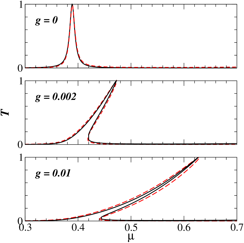
Figure 13: (color online) Transmission spectra of the double barrier potential at $g=0$ (upper panel), $g=0.002$ $\hbar\omega a_{\perp}$ (middle panel), and $g=0.01$ $\hbar\omega a_{\perp}$ (lower panel). The solid line shows the transmissions of all scattering states, calculated by the “stationary” method based on Eq. (17), that exist at the incident current $j_{i}=1\,\omega$ of the matter-wave beam. The dashed line is obtained from self-consistent solutions of Eq. (81) at $j_{i}=1\,\omega$, which are inserted in the expression (80) for the nonlinear transmission coefficient. The good agreement confirms the one-to-one correspondence between quasi-bound states of the atomic quantum dot and resonance peaks in the transmission spectrum ($\mu$ in units of $\hbar\omega$)

It is worthwhile to note that self-consistent solutions of the quasi-bound populations can also be found in a different way, namely by iteratively inserting approximate expressions for $N_{b}$ into the right-hand side of Eq. (81) starting with $N_{b}=0$. This approach would effectively mimic the quasi-stationary propagation of a Bose-Einstein condensate through the initially empty quantum dot. In agreement with the time-dependent propagation approach based on the inhomogeneous Gross-Pitaveskii equation (see Sec. II.3), only the lowest branch of the distorted resonance peak is populated in this way. This again underlines that the framework used in this section is intrinsically suited to take into account time-dependent effects and might therefore be used to predict the outcome of specific propagation processes.

IV Conclusion

We have presented analytical and numerical results for steady and time-dependent flows of repulsively interacting Bose condensed atoms through mesoscopic waveguide structures. To this end, we described a theoretical framework that is suitable to study transport and scattering processes in the 1D mean-field regime. In this context we introduced a non-perturbative method to extend the concept of transmission and reflection coefficients to nonlinear wave equations. On the other hand, to predict the behavior of the condensate flow under realistic experimental conditions, it is necessary to study time-dependent transport processes. We developed for this purpose a numerical method based on integrating the time-dependent Gross-Pitaevskii equation in presence of a source term that simulates the coupling of the waveguide to a reservoir from which a quasi-stationary flow of condensate is smoothly released into the guide.

The approach was first applied to the transport through a single quantum point contact, where we found as a main result that an increasing nonlinearity leads to a distinct reduction of the transmission. Much more complex behavior was found for the condensate flow through a double barrier potential. Here, the atom-atom interaction induces a bistability phenomenon of the transmitted flux in the vicinity of resonances, which manifests as a strong distortion of the transmission peaks. By means of the time-dependent integration scheme, we demonstrated that resonant transport will consequently be suppressed in a realistic propagation process. However, as we showed in Ref. PauRicSch05PRL , a suitable variation of the external potential during the propagation process can enhance the flow to reach a near-resonant state on finite time scales. Finally, an analytical description of the transport problem through the double barrier was developed, which establishes a clear link between the nonlinear signatures of the transmission spectra and the properties of the self-consistent quasi-bound states of the quantum dot. Similar results were recently obtained in Ref. RapKor07 as well.

Our numerical approach based on the inhomogeneous time-dependent Gross-Pitaevskii equation can be straightforwardly generalized to describe scttering processes in multidimensional geometries. It can certainly be applied also to more complex scattering potentials, involving more than two barriers. In that case, however, we do not expect that the calculation always converges towards a stationary scattering state, even if the source amplitude in the inhomogeneous Gross-Pitaevskii equation is varied on a very long time scale. This was demonstrated in our study on the transport of Bose-Einstein condensates through one-dimensional disorder, where we found that randomly generated disorder potentials of finite range will generally give rise to permanently time-dependent scattering processes at finite interaction, as long as the length of the disorder region exceeds a critical interaction-dependent value PauO05PRA ; Pau07PRL . Interestingly, this cross-over between quasi-stationary and time-dependent scattering, arising for disorder samples with lengths below and above this critical value respectively, correlates with a transition from an exponential (Anderson-like) to an algebraic decrease of the average transmission with the sample length PauO05PRA , which indicates that the depletion of the condensate during the propagation process might play a prominent role there. We note in this context that the effect of depletion can to a certain extent be accounted for within the framework of our approach, namely through the implementation of the microscopic quantum dynamics approach introduced by Köhler and Burnett Koe02PRA in combination with an external source Tom .

The results that were obtained in this work are related to other fields of nonlinear physics as well, such as nonlinear optics Vau96PRA and the electronic transport through quantum wells Goldman87 ; Azbel99 , where similar observations on resonant transport were made. In the context of Bose-Einstein condensates, the realization of a quasi-stationary flux of interacting matter waves though scattering potentials that are defined on microscopic length scales still represents a formidable experimental challenge. There are, however, promising advances in this direction, such as the atom-laser-like injection of a condensate into an optical waveguide Gue06PRL as well as the scattering of a stationary condensate in presence of a moving obstacle Engels . Such advances should, in combination with detection techniques for single atoms Teper06 ; Haase06 (which would allow one to measure very low transmissions), make it possible to experimentally investigate the role of interaction in mesoscopic transport processes from a new perspective, namely the one of cold bosonic atoms.

Appendix A

In this appendix we describe the numerical integration procedure of the time-dependent Gross-Pitaevskii equation and the implementation of the source term into this integration scheme. We consider the equation of motion (in the following we set for simplicity $\hbar=1$, $m=1$)

$$i\frac{\partial}{\partial t}\psi(x,t)=H(x,t)\psi(x,t),$$ (83)

with the effective nonlinear Hamiltonian

$$H(x,t)\equiv-\frac{1}{2}~{}\frac{\partial^{2}}{\partial x^{2}}+V(x)+g|\psi(x,t)|^{2},$$ (84)

which we want to integrate for a given initial state $\psi(x,t_{0})$ of the condensate. In order to compute the time evolution of the condensate wave function $\psi(x,t)$ for $t>t_{0}$, we subdivide the time interval $t-t_{0}$ into $n$ discrete time steps of the size $\Delta t=(t-t_{0})/n$, and use an implicit Crank-Nicholson integration scheme NumRec to propagate the wavefunction from one time step to the next one. The effective time evolution operator $\mathcal{U}$ for one discrete time step $\Delta t$ is then given by Ames

$${\mathcal{U}}(t+\Delta t,t)\equiv\frac{1}{1+\frac{i}{2}H(x,t)\Delta t}\left[1-\frac{i}{2}H(x,t)\Delta t\right].$$ (85)

The representation (85) of $\mathcal{U}$ is unitary and thus conserves the norm of the wave function $\psi$. The implicit integration scheme for the wave function reads then

$$\left(1+\frac{i\Delta t}{2}H\right)\psi(x,t+\Delta t)=\left(1-\frac{i\Delta t}{2}H\right)\psi(x,t).$$ (86)

We expand the wave function on a discrete lattice with $N$ lattice sites by introducing the grid basis

$$\chi_{j}\equiv\begin{cases}1:x_{j}-\frac{1}{2}\Delta x\leqslant x<x_{j}+\frac{1}{2}\Delta x\\ 0:\text{otherwise},\end{cases}$$ (87)

with $\Delta x\equiv(x_{min}-x_{max})/N$. Here, $x_{min}$ and $x_{max}$ are the boundaries of the finite grid. The wave function then reads

$$\psi(x,t_{n})=\sum\limits_{j=1}^{N}\psi_{j}^{n}\chi_{j},$$ (88)

where $\psi^{n}_{j}\equiv\psi(x_{j},t_{n})$ is value of the wave function at the position $x_{j}$ of the $j$’th lattice site (the index $n$ labels the discrete times, $t_{n}=t_{0}+n\Delta t$). Using the finite-difference representation for the kinetic part of $H(x,t)$, we find

$$\left(1\pm\frac{i\Delta t}{2}H\right)\psi(x_{j},t_{n})\simeq\psi_{j}^{n}\pm\frac{i\Delta t}{2}\times$$ (89)

$$\times\left[-\frac{\psi_{j+1}^{n}-2\psi_{j}^{n}+\psi_{j-1}^{n}}{2\,\Delta x^{2}}+V_{j}\psi_{j}^{n}+g|\psi_{j}^{n}|^{2}\psi_{j}^{n}\right]\qquad$$

with $V_{j}\equiv V(x_{j})$. By introducing $\vec{\psi}^{n}=\left(\psi_{1}^{n}...\psi_{j}^{n}...\psi_{N}^{n}\right)^{T}$, the lattice representation of Eq. (86) finally reads

$${\bf D}_{2}\vec{\psi}^{n+1}={\bf D}_{1}\vec{\psi}^{n}\quad\Leftrightarrow\quad\vec{\psi}^{n+1}={\bf D}_{2}^{-1}{\bf D}_{1}\vec{\psi}^{n}\,,$$ (90)

where we define

$${\bf D}_{1}\equiv\left[\left(1-\frac{i\Delta t}{2}H\right)\right],\ {\bf D}_{2}\equiv\left[\left(1+\frac{i\Delta t}{2}H\right)\right],$$ (91)

and the $N\times N$ matrix representation of ${\bf D}_{1,2}$ reads

$${\bf D}_{1,2}=\begin{pmatrix}\ddots&\ddots&\ddots&&&&\\ &\pm\alpha&1\mp\beta_{j-1}&\pm\alpha&&&\\ &&\pm\alpha&1\mp\beta_{j}&\pm\alpha&&\\ &&&\pm\alpha&1\mp\beta_{j+1}&\pm\alpha&\\ &&&&\ddots&\ddots&\ddots\end{pmatrix},$$

with

$$\alpha\equiv\frac{i\Delta t}{4\Delta x^{2}},\ \ \beta_{j}\equiv\frac{i\Delta t}{2}\left(\frac{1}{\Delta x^{2}}+V_{j}+g|\psi_{j}^{n}|^{2}\right).$$ (92)

Hence, the integration of Eq. (83) reduces to the solution of a system of linear equations with a tridiagonal matrix.

So far, our integration scheme uses the value of $\psi^{n}$ at the beginning of the integration step. This neglects the fact that the effective Hamiltonian (84) is implicitly time-dependent due to the presence of the nonlinear term $g|\psi(x,t)|^{2}$. Thus, it would be appropriate to use a more precise estimate for this nonlinear term, which is somehow averaged over the timestep $\Delta t$ leading from $t_{n}$ to $t_{n+1}$. This problem can be handled by using a predictor-corrector-like scheme which was already successfully applied in Cerbo . In this scheme, each integration step is done twice: First, we propagate the wave function from time $t_{n}$ to time $t_{n+1}$ using $\psi^{n}$ in the nonlinear term, in order to obtain a predicted wave function $\tilde{\psi}^{n+1}$. Then, we repeat this integration step but using now the averaged value $\frac{1}{2}[\psi^{n}+\tilde{\psi}^{n+1}]$ in the nonlinear term, yielding a corrected wave function $\psi^{n}$.

Now we consider the presence of the source term. The equation of motion reads therefore

$$i\frac{\partial}{\partial t}\psi(x,t)=H(x,t)\psi(x,t)+S(t)\exp(-i\mu t)\,\delta(x).$$ (93)

Working with a grid representation of the wave function, it is convenient to approximate the $\delta$-function by

$$R(x)=\frac{1}{\Delta x}\left[\Theta(x+\Delta x/2)-\Theta(x-\Delta x/2)\right],$$ (94)

where $\Theta$ is the Heavyside step function. Before including the source term to the finite difference scheme, we estimate the error that is introduced by this approximation. To this end, we study the steady-state solutions of the wave equation

$$i\frac{\partial\psi}{\partial t}-\left[-\frac{1}{2}\frac{\partial^{2}}{\partial x^{2}}+V_{\|}(x)+g|\psi|^{2}\right]\psi=S_{0}~{}R(x)\;,$$ (95)

that are obtained in the limit $t\to\infty$. The Green function that is associated with the stationary equivalent of Eq. (95) is given by

$$G(x-x^{\prime})=\frac{S_{0}}{ik}\;e^{ik|x-x^{\prime}|}$$ (96)

with $k=\sqrt{2(\mu-gn)}$ (see Sec. II.4, Eq. (46) ). Hence, the ansatz

$$\psi_{{}_{R}}(x)=\int_{-\infty}^{+\infty}dx^{\prime}\,\frac{S_{0}}{ik}e^{ik|x-x^{\prime}|}\,R(x^{\prime})$$ (97)

yields a solution $\psi_{{}_{R}}(x)$ of Eq. (95). Evaluating this integral yields

$$\psi_{{}_{R}}(x)=\frac{2S_{0}}{ik^{2}\Delta x}\left\{\begin{array}[]{r@{\; : \;}l}\displaystyle e^{-ikx}\sin(k\Delta x/2)&\displaystyle x<-\frac{\Delta x}{2}\\ \displaystyle 1-e^{ik\Delta x/2}\cos(kx)&\displaystyle|x|<\frac{\Delta x}{2}\\ \displaystyle e^{ikx}\sin(k\Delta x/2)&\displaystyle x>\frac{\Delta x}{2}\end{array}\right.$$ (98)

which converges towards Eq. (96) in the limit $\Delta x\to 0$. The result (98) can serve as an estimate for the relative error $\mathcal{F}$ that is done by approximating $\delta(x)$ with $R(x)$: we obtain

$${\mathcal{F}}=1-\frac{2\sin(k\Delta x/2)}{k\Delta x}\simeq\frac{k^{2}\Delta x^{2}}{24}\ \text{if}\ \frac{k\Delta x}{2}\ll 1.$$ (99)

The relative error therefore scales quadratically with the grid spacing $\Delta x$ and becomes negligible for reasonably small values of $\Delta x$.

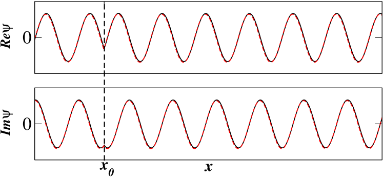
Figure 14: (color online) Real and imaginary parts (black solid lines) of the steady-state plane-wave solution obtained by integrating the time-dependent Gross-Pitaevskii equation with the numerical source term (94) using the time step $\Delta t=\hbar/(50\mu)$ and the grid spacing $\Delta x=\lambda/20$ with $\lambda=2\pi/k$ the wavelength of the condensate. An excellent agreement with the exact analytical result (95) (red dashed lines) is found. The source is located at the position $x=x_{0}$.

The above considerations justify the implementation of the source term at the position $x_{j^{\prime}}$ through the discretized form

$$S_{j}^{n}=S(t_{n})\exp({-i\mu t_{n}})\,\delta_{j,j^{\prime}}\,,$$ (100)

where $\delta_{j,j^{\prime}}=1$ if $j=j^{\prime}$ and $0$ otherwise. In the presence of the source term, Eq. (90) is modified and reads

$${\bf D}_{2}\vec{\psi}^{n+1}+\vec{b}^{n}={\bf D}_{1}\vec{\psi}^{n}\Leftrightarrow\vec{\psi}^{n+1}={\bf D}_{2}^{-1}({\bf D}_{1}\vec{\psi}^{n}-\vec{b}^{n}),$$

where the components of the vector $\vec{b}^{n}$ are given by

$$b_{j}^{n}=\frac{i\Delta t}{2}\left(S_{j^{\prime}}^{n}+S_{j^{\prime}}^{n+1}\right)\,\delta_{j,j^{\prime}}.$$ (101)

In Fig. 14, we compare the exact result (95) to the numerically computed plane-wave solution that is obtained in the limit $t\to\infty$ by simulating the gradual filling of a waveguide without scattering potential, $V_{\|}(x)\equiv 0$. Indeed, we find an excellent agreement between the numerical result and the exact plane-wave solution (95) if we choose, e.g., $\Delta x=\lambda/20$ (with the wavelength $\lambda=2\pi/k$) and $\Delta t=\hbar/(50\mu)$.

It is worthwhile to mention that in the presence of strong nonlinearities (for values of $g$ considerably larger than in this paper) and strong backreflection, a nonlinear back-action between the reflected matter wave and the source term can occur. As a consequence, the transmitted current depends not only on the source amplitude $S_{0}$ but also on the position of the source. In such a situation, it is advisable to implement the adiabatic transition scheme that is displayed in Fig. 3 where $g$ vanishes in the far-upstream region. By positioning the source term there and by choosing a sufficiently large transition region, one can avoid this nonlinear back-action and ensure that the wave function is adiabatically conveyed from a linear wave to a nonlinear scattering state obeying the Gross-Pitaevskii equation .

Appendix B

In the numerical treatment of time-dependent scattering processes in open quantum systems, one often encounters the problem of defining physically meaningful boundaries at the edges of the computational domain. The naive, straightforward expansion of the wave function on a finite spatial grid generally leads to an artificial backscattering of the wave function from the boundaries of the grid, which makes it impossible to simulate infinitely extended scattering states. This problem can be circumvented by introducing complex absorbing potentials in the vicinity of the grid boundaries (see, e.g., Ref. MoiO04JPB ), which should be designed such that they absorb the outgoing flux as best as possible without affecting the dynamics inside the scattering region. An alternative method, which was introduced by Shibata for the linear Schrödinger equation Shibata , consists in the definition of absorbing boundary conditions (ABC) at the edges of the grid, which are formulated in order to perfectly match outgoing plane waves with a specified dispersion relation. This method is particularly suited for quasi-stationary propagation processes where the outgoing part of the wave function is well described by a plane monochromatic wave. We show in this Appendix how this approach can be numerically implemented, and how the effect of a moderate nonlinearity in the Gross-Pitaevskii equation can be taken into account.

We first discuss the absorbing boundary conditions for the Schrödinger equation (with $\hbar=1$ and $m=1$)

$$i\frac{\partial}{\partial t}\psi(x,t)=\left(-\frac{1}{2}\frac{\partial^{2}}{\partial x^{2}}+V_{e}\right)\psi(x,t),$$ (102)

where $V_{e}$ is a constant potential which is independent of the position $x$. This equation admits plane-wave solutions $\psi(x,t)=Ae^{-i(\mu t-kx)}$ satisfying the dispersion relation

$$k=\pm\sqrt{2(\mu-V_{e})}.$$ (103)

The “$+$” and “$-$” branches of Eq. (103) correspond to plane waves that propagate to the right- and left-hand side, respectively. Thus, the ABC should satisfy the dispersion relation given by the “$+$” branch of Eq. (103) at the right boundary and the “$-$” branch at the left boundary of the grid.

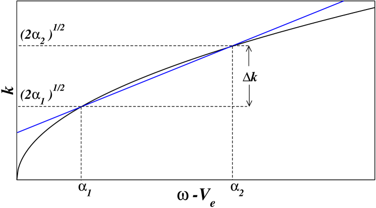
Figure 15: (color online) The positive branch of the dispersion relation of a plane wave (black line) is approximated by a linear function (straight blue line). The parameters $\alpha_{1},\alpha_{2}$ are chosen such that the wave numbers of the plane waves to be absorbed lie within the momentum interval $\Delta k$.

We derive now so called “one-way wave equations” on the basis of the dispersion relation (103), which we will implement at the boundaries of the grid and which locally allow for wave propagation only in the outgoing direction. To this end, we make use of the duality relations

$$\frac{\partial}{\partial t}\Longleftrightarrow-i\mu,\quad\frac{\partial}{\partial x}\Longleftrightarrow ik$$ (104)

which is going to be inserted into the dispersion relation (103). Unfortunately Eq. (103) is nonlinear in $\mu$ and cannot be straightforwardly converted into a linear differential equation. To circumvent this problem, we approximate Eq. (103) in the vicinity of the chemical potential of the wave to be absorbed by the linear function

$$k=\pm\frac{\sqrt{2\alpha_{2}}-\sqrt{2\alpha_{1}}}{\alpha_{2}-\alpha_{1}}~{}\mu~{}\pm\frac{\alpha_{2}\sqrt{2\alpha_{1}}-\alpha_{1}\sqrt{2\alpha_{2}}}{\alpha_{2}-\alpha_{1}}$$ (105)

(see Fig. 15). The parameters $\alpha_{1},\alpha_{2}$ are chosen such that Eq. (105) is a good approximation to the dispersion relation (103) within the interval $\Delta k\equiv\sqrt{2\alpha_{2}}-\sqrt{2\alpha_{1}}\,$ around the central wave number $\frac{1}{2}(\sqrt{2\alpha_{2}}+\sqrt{2\alpha_{1}})$. By use of the duality relations (104), Eq. (105) is transformed into the one-way wave equation

$$i\frac{\partial\psi}{\partial t} = \left(-i\frac{1}{g_{1}}\frac{\partial}{\partial x}+V_{e}-\frac{g_{2}}{g_{1}}\right)\psi,$$ (106)

with

$$g_{1} \equiv \pm\frac{\sqrt{2\alpha_{2}}-\sqrt{2\alpha_{1}}}{\alpha_{2}-\alpha_{1}},$$

$$g_{2} \equiv \pm\frac{\alpha_{2}\sqrt{2\alpha_{1}}-\alpha_{1}\sqrt{2\alpha_{2}}}{\alpha_{2}-\alpha_{1}}.$$ (107)

Implementing these one-way wave equations at the boundaries of the grid (see below) leads to a very good absorption of plane waves with wave numbers $k$ satisfying $\sqrt{2\alpha_{1}}\lesssim k\lesssim\sqrt{2\alpha_{2}}$. In Ref. Shibata it was demonstrated that also wave packets of the form $\psi\equiv\sum_{j}A_{i}\exp(ik_{j}x)$ can be absorbed if all wave numbers in this superposition lie within the above interval.

It is straightforward to see that the one-way equations (106) absorb plane waves also in the presence of the nonlinear term $g|\psi|^{2}$. This is evident for the special case of a constant density: $\psi(x,t)=\sqrt{n}\exp(-i\mu t/\hbar\pm ikx)$ with the dispersion relation

$$k=\pm\sqrt{2(\mu-gn)}.$$ (108)

is obviously a solution of the Gross-Pitaevskii equation. A comparison of Eq. (108) with Eq. (103) reveals that the term $gn$ can be identified as a constant effective potential. Hence we set $V_{e}\equiv gn$ for a proper absorption of the plane wave.

We now generalize this result for plane waves whose parameters are slowly varying in time and position. This case is of high relevance for our work since the gradual filling of the guide with matter waves leads to the population of a scattering state whose outgoing parts, which have to be absorbed at the boundaries of the grid, exhibit slowly varying amplitudes and phases. We consider

$$\psi(x,t)=A(x,t)e^{-i\mu t\pm iS(x,t)}$$ (109)

where $A(x,t)$ and $S(x,t)$ represent the local amplitude and phase, respectively, of the wave function. Locally, at position $x=x_{0}$, we can expand the phase according to

$$S(x,t)=S(x_{0},t)+k(x_{0},t)(x-x_{0})+{\mathcal{O}}[(x-x_{0})^{2}]$$ (110)

with $k(x_{0},t)\equiv\partial_{x}S(x,t)|_{x=x_{0}}$ In the limiting case where $A(x,t)$ and $S(x,t)$ vary on time and length scales that are considerably larger than $1/\mu$ and $1/k(x_{0},t)$, respectively (for $x\simeq x_{0}$ and for all times $t$), Eq. (109) locally takes the form of a plane wave with a slowly varying amplitude and wave number. Under this condition, we find at a given position $x_{0}$ at any time the local dispersion relation

$$k(x_{0},t)=\pm\sqrt{2(\mu-gn(x_{0},t))}.$$ (111)

with $n(x_{0},t)=|A(x_{0},t)|^{2}$. Hence, $k(x_{0},t)$ parametrically depends on $t$ via the condensate density at the position $x_{0}$ which is supposed to be at the boundary of the grid. By adjusting the values of $\alpha_{1}$ and $\alpha_{2}$ such that $\sqrt{2\alpha_{1}}\lesssim k(x_{0},t)\lesssim\sqrt{2\alpha_{2}}$ is satisfied for all times $t$, the wave $\psi$ is absorbed at the edge of the lattice.

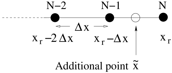
Figure 16: Sketch of the right lattice boundary. The additional point at position $\tilde{x}$ allows for a proper implementation of the absorbing boundary conditions in a grid representation of the wave function.

We now outline how to incorporate the ABC into the lattice representation (88) of the wave function. Here we consider exemplarily the right-hand side boundary $x_{r}=x_{N}$ of the grid, where the wave function has to obey Eq. (106) with the upper ($+$) sign in the definition (B) of the prefactors. The idea is now to replace the equation for the boundary component $\psi_{N}^{n}$ of the state vector $\vec{\psi}^{n}$, i.e. the last component in the equation (90), by the finite-difference version of the one-way wave equation (106). To this end, we need a finite-difference expression for the derivative $\partial_{x}\psi(x,t)|_{x=x_{r}}$ at the grid boundary. Since $x_{r}$ is the last grid point, this expression can only be obtained in an asymmetric way with respect to $x_{r}$, namely through the difference between $\psi(x_{r},t)$ and $\psi(x_{r}-\Delta x,t)$. This would lead to the equation

$$\frac{i}{\Delta t}[\psi(x_{r},t+\Delta t)-\psi(x_{r},t)]=\left(V_{e}-\frac{g_{2}}{g_{1}}\right)\psi(x_{r},t)$$ (112)

$$\qquad\qquad\quad-\frac{i}{g_{1}}\frac{\psi(x_{r},t)-\psi(x_{r}-\Delta x,t)}{\Delta x}\qquad$$

which was also used in Ref. Shibata .

The asymmetric structure of Eq. (112) introduces a small but systematic error in the propagation of the wave function, since the value and the derivate of $\psi$ are, strictly speaking, computed at different positions, namely at $x_{r}$ and at the intermediate point $\tilde{x}=x_{r}-\Delta x/2$, respectively. This problem can be circumvented by replacing Eq. (112) with the analogous equation for the wave function $\psi(\tilde{x},t)$ evaluated at this intermediate point $\tilde{x}$ (see Fig. 16). There we have

$$\left.\frac{\partial}{\partial x}\psi(x,t)\right|_{x=\tilde{x}}\simeq\frac{\psi(x_{r},t)-\psi(x_{r}-\Delta x,t)}{\Delta x}\,.$$ (113)

as “exact” (i.e., symmetric) finite-difference expression for the derivative, and the value of the wave function at this additional point is obtained through

$$\psi(\tilde{x},t)\simeq\frac{1}{2}\left[\psi(x_{r},t)+\psi(x_{r}-\Delta x,t)\right].$$ (114)

Inserting these expressions (113) and (114) into Eq. (106) leads to a symmetric finite-difference equation for $\psi(x_{r},t)$ and $\psi(x_{r}-\Delta x,t)$ where the value of the wave function at the auxiliary point $\tilde{x}$ does not explicitly appear any longer. In the grid representation, this finite-difference equation reads

$$\frac{i}{2\Delta t}(\psi_{N}^{n+1}+\psi_{N-1}^{n+1}-\psi_{N}^{n}-\psi_{N-1}^{n})=\frac{-i}{g_{1}\Delta x}(\psi_{N}^{n}-\psi_{N-1}^{n})$$ (115)

$$\qquad\qquad\qquad+\frac{1}{2}\left(V_{e}-\frac{g_{2}}{g_{1}}\right)\left(\psi_{N}^{n}+\psi_{N-1}^{n}\right).\qquad\qquad$$

Eq. (115) allows for a straightforward incorporation into the matrix representation (91): the modified matrices ${\bf D}_{1,2}$ read at the right-hand side edge of the numerical grid

$${\bf D}_{1} \equiv \begin{pmatrix}&\ddots&\ddots&\ddots&&\\ &&\alpha&1-\beta_{N-2}&\alpha&\\ &&&\alpha&1-\beta_{N-1}&\alpha\\ &&&&\gamma_{3}&\gamma_{4}\end{pmatrix},$$

$${\bf D}_{2} \equiv \begin{pmatrix}&\ddots&\ddots&\ddots&&\\ &&-\alpha&1+\beta_{N-2}&-\alpha&\\ &&&-\alpha&1+\beta_{N-1}&-\alpha\\ &&&&\gamma_{1}&\gamma_{2}\end{pmatrix}$$ (116)

where we define

$$\gamma_{1} \equiv \gamma_{2}\equiv\frac{i}{2\Delta t},$$

$$\gamma_{3} \equiv \frac{i}{2\Delta t}+\frac{i}{g_{1}\Delta x}+\left(V_{e}-\frac{g_{2}}{g_{1}}\right),$$

$$\gamma_{4} \equiv -\frac{i}{2\Delta t}-\frac{i}{g_{1}\Delta x}+\left(V_{e}-\frac{g_{2}}{g_{1}}\right).$$ (117)

The main cause for artificial backreflection in presence of the above boundary conditions comes from the approximate nature of the finite-difference evaluations (113) and (114). Clearly, these approximations become better with decreasing grid spacing $\Delta x$, which means that a reduction of the grid spacing should lead to a more efficient absorption of the outgoing flux. In practice, we find for grid spacings of the order of $\Delta x=\lambda/30$ (with $\lambda=2\pi/k$ the wavelength of the condensate) that the relative amplitude of artificial backreflections from the grid boundaries is below $1\%$. We note that the amount of backreflection that is accumulated during the numerical propagation process would, at the same value of the grid spacing $\Delta x$, be considerably larger if the asymmetric version (112) of the one-way wave equation was used instead of Eq. (115).

References

- (1) T. Anker, M. Albiez, R. Gati, S. Hunsmann, B. Eiermann, A. Trombettoni, and M. K. Oberthaler, Phys. Rev. Lett. 94, 020403 (2005).
- (2) Y. Shin, C. Sanner, G.-B. Jo, T. A. Pasquini, M. Saba, W. Ketterle, D. E. Pritchard, M. Vengalattore, M. Prentiss, Phys. Rev. A 72, 021604 (2005).
- (3) T. Schumm, S. Hofferberth, L. M. Andersson, S. Wildermuth, S. Groth, I. Bar-Joseph, J. Schmiedmayer, and P. Krüger, Nature Physics 1, 57 (2005).
- (4) A. Günther, S. Kraft, M. Kemmler, D. Koelle, R. Kleiner, C. Zimmermann, and J. Fortágh, Phys. Rev. Lett. 95, 170405 (2005).
- (5) R. Folman, P. Krüger, D. Cassettari, B. Hessmo, T. Maier, and J. Schmiedmayer, Phys. Rev. Lett. 84, 4749 (2000).
- (6) W. Hänsel, P. Hommelhoff, T. W. Hänsch, and J. Reichel, Nature 413, 498 (2001).
- (7) H. Ott, J. Fortágh, S. Kraft, A. Günther, D. Komma, and C. Zimmermann, Phys. Rev. Lett. 91, 040402 (2003).
- (8) J. H. Thywissen, R. M. Westervelt, and M. Prentiss, Phys. Rev. Lett. 83, 3762 (1999).
- (9) I. Carusotto and G. C. La Rocca, Phys. Rev. Lett. 84, 399 (1999).
- (10) I. Carusotto, Phys. Rev. A 63, 023610 (2001).
- (11) T. Paul, K. Richter, and P. Schlagheck, Phys. Rev. Lett. 94, 020404 (2005).
- (12) K. Rapedius, D. Witthaut, and H. J. Korsch, Phys. Rev. A 73, 033608 (2006).
- (13) T. Paul, P. Leboeuf, N. Pavloff, K. Richter, and P. Schlagheck, Phys. Rev. A 72, 063621 (2005).
- (14) T. Paul, P. Schlagheck, P. Leboeuf, and N. Pavloff, Phys. Rev. Lett. 98, 210602 (2007).
- (15) N. Bilas and N. Pavloff, Phys. Rev. Lett. 95, 130403 (2005).
- (16) W. Guerin, J.-F. Riou, J. P. Gaebler, V. Josse, P. Bouyer, and A. Aspect, Phys. Rev. Lett. 97, 200402 (2006).
- (17) I. Bloch and T. W. Hänsch, and T. Esslinger, Phys. Rev. Lett. 82, 3008 (1999).
- (18) C. Menotti and S. Stringari, Phys. Rev. A 66, 043610 (2002).
- (19) P. Leboeuf and N. Pavloff, Phys. Rev. A 64, 033602 (2001).
- (20) P. Leboeuf, N. Pavloff, and S. Sinha, Phys. Rev. A 68, 063608 (2003).
-
(21)
L. Pitaevskii, and S. Stringari,
Bose-Einstein Condensa-
tion, (Oxford University Press, Oxford 2003). - (22) F. Dalfovo S. Giorgini L. P. Pitaevskii and S. Stringari, Rev. Mod. Phys. 71, 463 (1999).
- (23) Y. Castin and R. Dum, Phys. Rev. Lett. 77, 5315 (1996).
- (24) A. D. Jackson G. M. Kavoulakis, and C. J. Pethick, Phys. Rev. A 58, 2417 (1998).
- (25) D. S. Petrov, G. V. Shlyapnikov, and J. T. M. Walraven, Phys. Rev. Lett. 85, 3745 (2001).
- (26) V. Dunjko, V. Lorent, and M. Olshanii, Phys. Rev. Lett. 86, 5413 (2001).
- (27) M. Olshanii, Phys. Rev. Lett. 81, 938 (1998).
- (28) J. H. Thywissen, M. Olshanii, G. Zabow, M. Drndic, K. S. Johnson, R.M. Westervelt, M. Prentiss, Eur. Phys. J. 7, 361 (1999).
- (29) For a given value of , we numerically compute the ground state of Eq. (8) by means of imaginary-time propagation ChiSucTos00PRE and obtain in this way the corresponding value of .
- (30) S. A. Gredeskul and Y. S. Kivshar Phys. Rep 216, 1 (1992).
- (31) R. Knapp, G. Papanicolaou, and B. White J. Stat. Phys. 63, 567 (1991).
- (32) T. Shibata, Phys. Rev. B 43, 6760 (1990).
- (33) Obviously, numerical convergence towards dynamically unstable scattering states is not possible.
- (34) P. Engels and C. Atherton, arXiv:0704.2427 (2007).
- (35) A multilayer chip geometry might be employed to avoid decoherence and fragmentation effects that would result from the near vicinity of the condensate to the wires creating the magnetic waveguide.
- (36) D. Ferry and S. Goodnick. Transport in Nanostructures (Cambridge University Press, Cambridge, 1997).
- (37) For the peak becomes distorted towards lower values of .
- (38) R. W. Boyd, Nonlinear Optics (Academic Press, London, 1992).
- (39) V. J. Goldman, D. C. Tsui, and J. E. Cunningham, Phys. Rev. Lett. 58, 1256 (1987).
- (40) M. Y. Azbel’, Phys. Rev. B 59, 8049 (1999).
- (41) C. Mahaux and H. A. Weidenmüller, Shell-Model Approach to Nuclear Reactions (North-Holland, Amsterdam, 1969); J. J. M. Verbaarschot, H. A. Weidenmüller, and M. R. Zirnbauer, Phys. Rep. 129, 367 (1985).
- (42) H. Feshbach, Ann. Phys. (N.Y.) 5, 357 (1958); Ann. Phys. (N.Y.) 19, 287 (1962).
- (43) C. Viviescas and G. Hackenbroich, Phys. Rev. A 67, 013805 (2003).
- (44) N. Moiseyev, L. D. Carr, B. A. Malomed, and Y. B. Band, J. Phys. B 37, L193 (2004).
- (45) D. Witthaut, S. Mossmann, and H. J. Korsch, J. Phys. A 38, 1777 (2005).
- (46) L. D. Carr, M. J. Holland, and B. A. Malomed, J. Phys. B 38, 3217 (2005).
- (47) P. Schlagheck and T. Paul, Phys. Rev. A 73, 023619 (2006).
- (48) S. Wimberger, P. Schlagheck, and R. Mannella, J. Phys. B 39, 729 (2006), P. Schlagheck and S. Wimberger, Appl. Phys. B 86, 385 (2007).
- (49) K. Rapedius and H.-J. Korsch, arXiv:0706.2826 (2007).
- (50) T. Köhler and K. Burnett, Phys. Rev. A 65, 033601 (2002).
- (51) T. Ernst, T. Paul, and P. Schlagheck, in preparation.
- (52) M. Vaupel, K. Staliunas, and C. O. Weiss, Phys. Rev. A 54, 880 (1996).
- (53) Igor Teper, Yu-Ju Lin, and V. Vuletić, Phys. Rev. Lett. 97, 023002 (2006).
- (54) A.Haase, B.Hessmo and J.Schmiedmayer, Optics Letters, 31, 268 (2006).
- (55) W. H. Press, S. A. Teukolsky, W. T. Vetterling, and B. P. Flannery, Numerical Recipes in C++ (Cambridge University Press, Cambridge, 2002).
- (56) W. A. Ames, Numerical Methods for Partial Differential Equations, (Academic Press, New York, 1977).
- (57) E. Cerboneschi, R. Mannella, E. Arimondo, and L. Salasnich, Phys. Lett. A 249, 495 (1998).
- (58) M. L. Chiofalo S. Succi, and M. P. Tosi, Phys. Rev. E 62, 7438 (2000).