Magnetospheric Emissions from the Planet Orbiting $\tau$ Boo (catalog ): A Multi-Epoch Search

Abstract

All of the solar system gas giants produce electron cyclotron masers, driven by the solar wind impinging on their magnetospheres. Extrapolating to the planet orbiting $\tau$ Boo (catalog ), various authors have predicted that it may be within the detection limits of the 4-meter wavelength (74 MHz) system on the Very Large Array. This paper reports three epochs of observations of $\tau$ Boo (catalog ). In no epoch do we detect the planet; various means of determining the upper limit to the emission yield single-epoch limits ranging from 135 to 300 mJy. We develop a likelihood method for multi-epoch observations and use it to constrain various radiation properties of the planet. Assuming that the planet does radiate at our observation wavelength, its typical luminosity must be less than about $10^{16}$ W, unless its radiation is highly beamed into a solid angle $\Omega\ll 1$ sr. While within the range of luminosities predicted by various authors for this planet, this value is lower than recent estimates which attempt to take into account the stellar wind of $\tau$ Boo (catalog ) using the known properties of the star itself. Electron cyclotron maser emission from solar systems planets is beamed, but with characteristic solid angles of approximately 1 sr illuminated. Future long-wavelength instruments (e.g., the Long Wavelength Array and the Low Frequency Array) must be able to make typical flux density measurements on short time scales ($\approx 15$ min.) of approximately 25 mJy in order to improve these constraints significantly.

1 Introduction

The star $\tau$ Boo (catalog ) is an F6IV star located 15.6 pc away (Perryman et al., 1997) that is orbited by a planet with a minimum mass of 4.14 M_J (Jovian masses) orbiting in a 3.3 day period (semi-major axis of 0.047 AU, Butler et al., 1997).

By analogy to the “magnetic planets” in the solar system (Earth (catalog ), Jupiter (catalog ), Saturn (catalog ), Uranus (catalog ), and Neptune (catalog )), there have been various predictions that Jovian-mass extrasolar planets should also emit intense cyclotron maser emission at radio wavelengths (Zarka et al., 1997; Farrell et al., 1999; Zarka et al., 2001; Lazio et al., 2004; Stevens, 2005; Griessmeier et al., 2005; Zarka, 2006, 2007). Extrapolating empirical relationships based on the solar system planets, it is possible to make quantitative predictions for both the characteristic emission wavelength and radio luminosity for an extrasolar planet (Farrell et al., 1999; Lazio et al., 2004; Stevens, 2005; Griessmeier et al., 2005).

For the planet orbiting $\tau$ Boo (catalog ), these predictions are that its characteristic emission wavelength should be between about 5 and 7 meters (45 and 60 MHz) and that its radio luminosity would result in a flux density at the Earth (catalog ) between roughly 1 and 250 mJy (Lazio et al., 2004; Stevens, 2005; Griessmeier et al., 2005). The lower flux density estimates result from treating $\tau$ Boo (catalog ) as effectively a solar twin, while the higher estimates take into account its (higher) level of stellar activity resulting from it being younger than the Sun (Stevens, 2005; Griessmeier et al., 2005). In addition, for the solar system planets, variations within the level of solar activity can amplify the cyclotron maser emission process, producing radio luminosities (and therefore flux densities) 1–2 orders of magnitude above the nominal level.

Indirect evidence for extrasolar planetary magnetic fields comes in the form of modulations in the Ca II H and K lines of the stars HD 179949 (catalog HD) and $\upsilon$ And (catalog ), modulations that are in phase with the orbital periods of their planets with the smallest semi-major axes (Shkolnik et al., 2005). Though they monitored $\tau$ Boo (catalog ), no similar modulations were seen. Shkolnik et al. (2005) suggest that the Ca II line modulations result from energy transport related to the relative velocity between planet and the stellar magnetosphere. Any such Ca II line modulations for $\tau$ Boo (catalog ) would then be suppressed because the star’s rotation period is comparable to the planet’s orbital period ($\approx 3$ d, Catala et al., 2007). Suggestively, though, the polarization observations of Catala et al. (2007) do suggest a complex surface magnetic field topology for $\tau$ Boo (catalog ), consistent with a possible interaction with the planet’s magnetic field.

For the solar system planets, the cyclotron maser emission is fairly wideband with $\lambda/\Delta\lambda\sim 2$ ($\Delta\nu/\nu\sim 1/2$). The Very Large Array (VLA) is equipped with a 4-meter wavelength (74 MHz) receiving system. Images can be made with the VLA in its more extended configurations (A and B) with rms noise levels of approximately 100 mJy beam^-1. Thus, the radio emission from the planet may extend to wavelengths of 4 meters, and the planet may be detectable with current instrumentation.

This paper reports three epochs of 74 MHz observations of $\tau$ Boo (catalog ) with the VLA. In §2 we describe the observations; in §3 we analyze our observations both from the standpoint of the individual epochs as well as taken collectively and we make suggestions about the methodology for observations with future radio telescopes; and in §4 we present our conclusions.

2 Observations

Our observations were conducted on three epochs with the VLA in its more extended configurations. Table 1 summarizes various observational details. The use of the extended VLA configurations provided angular resolutions comparable to or better than 1′; such resolution is required to reduce the impact of source confusion. Dual circular polarization was recorded at all epochs, and the total bandwidth was 1.56 MHz, centered at 73.8 MHz.

Table 1: 74 MHz Observational Log

Epoch	Configuration	Duration	Beam	Image Noise Level
		(min.)	(″)	(mJy beam-1)
1999 June 8	D$\to$A	281	$30\times 29$	120
2001 January 19	B	175	$80\times 80$	110
2003 September 12	BnA	166	$32\times 21$	100

Post-processing of 4-m wavelength VLA data uses procedures similar to those at shorter wavelengths, although certain details differ. The source Cygnus A (catalog ) served as both the bandpass, flux density, and visibility phase calibrator. For two of the epochs (1999 June 8 and 2003 September 12), visibility phase calibration was performed in much the same manner as at shorter wavelengths, with the phases determined from Cygnus A (catalog ) transferred to the $\tau$ Boo (catalog ) data. Several iterations of hybrid mapping (imaging and self-calibration) then ensued. For the middle epoch, the data were acquired as part of the VLA Low-frequency Sky Survey (VLSS, Cohen et al., 2007). For these data, small “postage stamp” images of bright sources from the NRAO VLA Sky Survey (Condon et al., 1998) within the field of view were made every 1 min. The positions of the NVSS sources are determined at 20 cm, a wavelength at which the ionosphere should present only minor perturbations. The apparent positions at 4-meter wavelength were compared with the known positions from 20 cm. Low-order Zernicke polynomials were used to model the set of position offsets and thereby infer the phase corrections to be applied to the data. After applying these phase corrections, the full data set was imaged.

Two significant differences for the post-processing were the impact of radio frequency interference (RFI) and the large fields of view. In order to combat RFI, the data were acquired with a much higher spectral resolution than used for imaging. Excision of potential RFI is performed on a per-baseline basis for each visibility spectrum. For two of the epochs (1999 June 8 and 2003 September 12), RFI was identified and excised manually; for the second epoch (2001 January 19), RFI was identified and excised on an automated basis by fitting a linear function to each 10-s visibility spectrum and removing outlier channels. The large field of view (11° at 74 MHz) mean that the sky cannot be approximated as flat. In order to approach the thermal noise limit, we used a polyhedron algorithm (Cornwell & Perley, 1992) in which the sky is approximated by many two-dimensional “facets.”

Figures 1–3 present 74 MHz images of the field around $\tau$ Boo (catalog ) at the three epochs.

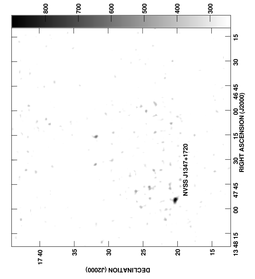
Figure 1: The field around $\tau$ Boo (catalog ) at 74 MHz for the epoch 1999 June 8. The grey scale flux range is linear between 240 ($2\sigma$) and 900 mJy beam^-1. The source in the lower left is NVSS J1347$+$1720 (catalog NVSS) and is used to assess the accuracy of our astrometry.

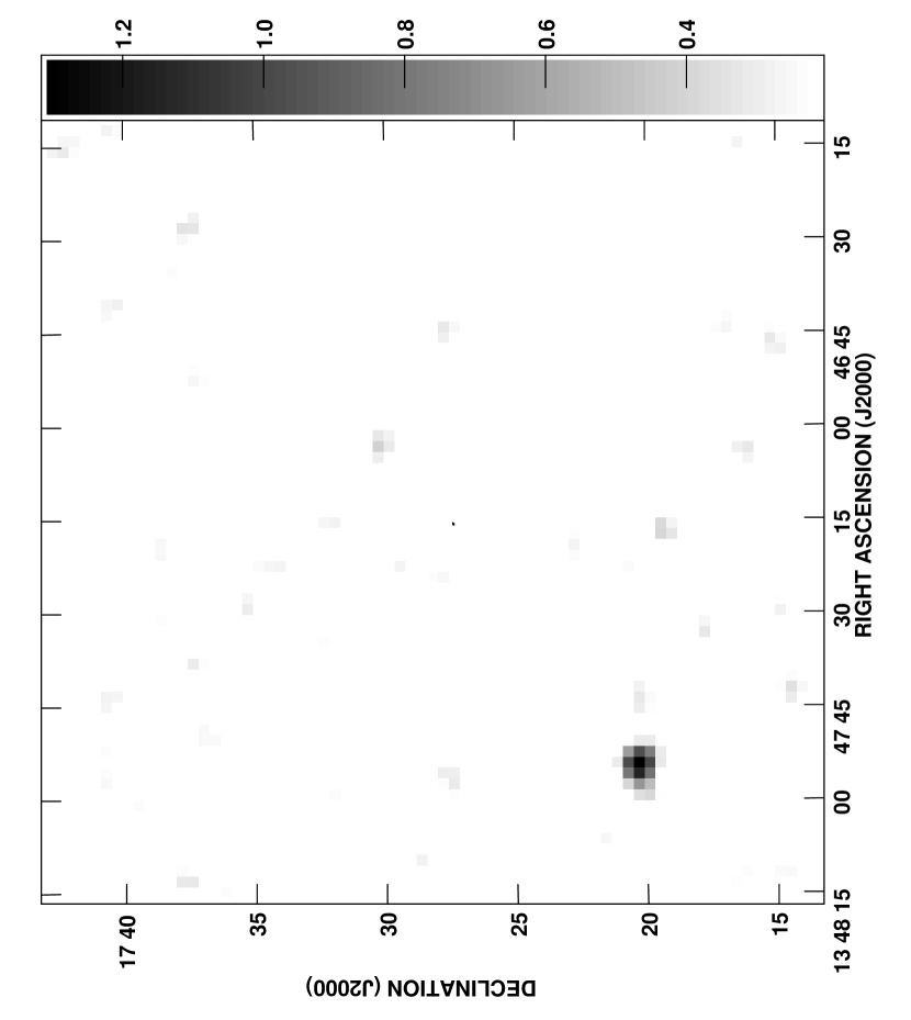
Figure 2: As for Figure 1 for the epoch 2001 January 19. The grey scale flux range is linear between 220 ($2\sigma$) and 1300 mJy beam^-1.

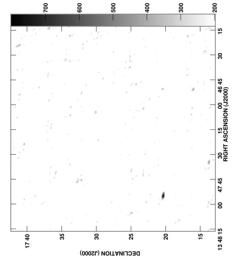
Figure 3: As for Figure 1 for the epoch 2003 September 12. The grey scale flux range is linear between 200 ($2\sigma$) and 800 mJy beam^-1.

3 Discussion and Analysis

We have used a number of different methods in order to assess the limits on the presence of any emission at the location of $\tau$ Boo (catalog ). We begin with an assessment of the astrometric accuracy of the images.

3.1 Astrometric Accuracy

Ionospheric phase fluctuations result in refractive shifts in the apparent positions of sources within the images. In all of the images (Figures 1–3) is the source NVSS J1347$+$1720 (catalog NVSS). The position of this source is determined at a shorter wavelength (20 cm or 1400 MHz) at which the ionospheric-induced position shifts are unimportant. For each epoch, we have fit an elliptical gaussian to NVSS J1347$+$1720 (catalog NVSS) and determined the position from that fit. Uncertainties, in either right ascension or declination, are between 0$\farcs$3 and 6″.

In addition, $\tau$ Boo (catalog ) has a measured proper motion of $\mu_{\alpha}=-480.34\pm 0.66$ mas yr^-1 and $\mu_{\delta}=54.18\pm 0.40$ mas yr^-1, measured in the epoch 1991.25 (Perryman et al., 1997). Over the decade between the epoch of the proper motion determination and the measurements reported here, we expect $\tau$ Boo (catalog ) to have moved by no more than about 5″. Adding these uncertainties in quadrature, we expect that the position of $\tau$ Boo (catalog ) in these images should be uncertain by no more than about 8″. The size of the beam (point spread function) ranges from about 25″ (epochs 1 and 3) to 80″ (epoch 2). We conclude that our astrometry is accurate to a fraction of a beam width.

3.2 Single-Epoch Limits on the Planetary Radio Emission

In no epoch do we detect statistically significant emission at the location of $\tau$ Boo (catalog ). Our first estimate for the upper limit to any emission from the planet orbiting $\tau$ Boo (catalog ) is obtained from the rms noise level in each image (Table 1). Because our astrometry is accurate to better than a beam width, we set an upper limit of $2.5\sigma$ at each epoch. The resulting upper limits are 250–300 mJy.

As a second means for setting an upper limit, we use the brightest pixel within a beam centered on the position of $\tau$ Boo (catalog ) to estimate the flux density of any possible radio emission from its planet. This estimate takes into account the background level determined by the mean brightness in a region surrounding the central beam. Upper limits determined in this manner range from 135 to 270 mJy.

As a final means for setting an upper limit, we have co-added (“stacked” or superposed epoch analysis) the three images, a technique has been used with great success to find weak sources in diverse data sets (e.g., sources contributing to the hard X-ray background, Worsley et al. 2005; intergalactic stars in galaxy clusters, Zibetti et al. 2005). Experience with 74 MHz images shows that the rms noise level in an image produced from the sum of $N$ images is $\sqrt{N}$ lower, as expected if the noise in the images is gaussian random noise. Obviously, by co-adding images, we will be less sensitive to a rare, large enhancement in the planetary radio emission caused by a temporary increase in the stellar wind flux, but we will be more sensitive to the nominal flux density, particularly for the higher estimates for the planet’s flux density (e.g., Stevens, 2005). The ($1\sigma$) noise level in the co-added image is 65 mJy beam^-1, a value consistent with that expected if the noise in all of the images is gaussian. We do not detect any source at the position of $\tau$ Boo (catalog ) at the level of 165 mJy ($2.5\sigma$).

Table 2 summarizes these limits. At any given epoch, the upper limits on radio emission at 74 MHz from the planet orbiting $\tau$ Boo (catalog ) range from an optimistic 135 mJy to, more conservatively, 300 mJy. On average, the planet’s flux density is not larger than 165 mJy. We convert these flux densities to luminosities assuming that the emission is broadband ($37\,\mathrm{MHz}=1/2$ of the observing frequency) and that the planet radiates into a solid angle of 1 sr (see below).

Table 2: 74 MHz $\tau$ Boo (catalog ) Observational Limits

Method	Epoch	Limit
		(mJy)	($\times 10^{16}$ W)
rms noise level	1999 June 8	300	2.6
	2001 January 19	275	2.4
	2003 September 12	250	2.1
brightest pixel	1999 June 8	270	2.3
	2001 January 19	134	1.1
	2003 September 12	189	1.6
stacked image	…	165	1.4

Note. — Luminosity limits adopt a distance of 15.6 pc and assume an emission bandwidth of 37 MHz ($=74\,\mathrm{MHz}/2$).

This planet does not transit its host star. While the planetary magnetosphere might be large, the typical emission altitude for an electron cyclotron maser for solar system planets is approximately 1–3 planetary radii. Thus, these limits should apply regardless of orbital phase.

3.3 Likelihood Estimates for Multi-Epoch Planetary Radio Observations

Earlier work by Bastian et al. (2000), Farrell et al. (2003), Ryabov et al. (2004), and Farrell et al. (2004) (and §3.2) reported non-detections from a single observation of a planet. (In addition, Yantis, Sullivan, & Erickson 1977 and Winglee, Dulk, & Bastian 1986 conducted blind searches for extrasolar planetary radio emission, but it is not clear that they observed any star now known to be orbited by a planet, and we believe that they observed each star for only a single epoch.) In addition, $\tau$ Boo (catalog ) has been observed at 150 MHz with the Giant Metrewave Radio Telescope (GMRT, Majid et al., 2006), the results from which will be reported elsewhere. Here we have reported non-detections from multiple observations of $\tau$ Boo (catalog ). Both in the context of these observations as well as from the standpoint of future observations, to what extent can multiple non-detections of a planet be used to place constraints on its radio emission?

The expected flux density for the radio emission from an extrasolar planet is (Farrell et al., 1999; Lazio et al., 2004)

$$S=\frac{P_{\mathrm{rad}}}{\Delta\nu\Omega D^{2}},$$ (1)

where $P_{\mathrm{rad}}$ is the luminosity or radiated power from the planet, $\Delta\nu$ is the emission bandwidth of the radiation, $\Omega$ is the solid angle into which the radiation is beamed, and $D$ is the distance of the planet (or its host star) from the Sun. In turn, the luminosity or radiated power and the emission bandwidth can be related to various planetary properties (e.g., mass and rotation rate of the planet). The standard practice has been to use empirical laws from the solar system to make predictions for $P_{\mathrm{rad}}$ and $\Delta\nu$.

Planetary radio emission has a characteristic wavelength $\lambda_{c}$ or frequency $\nu_{c}$, which is related to the cyclotron frequency at the lowest altitude at which emission is able to escape (Farrell et al., 1999). In turn, this characteristic wavelength is related to the magnetic moment or the magnetic field strength at the planet’s surface. The emission is typically broadband, with $\lambda_{c}/\Delta\lambda=\nu_{c}/\Delta\nu\sim 2$. In making predictions, it has been assumed that extrasolar planetary radio emission is comparably broadband, and, more importantly, that any observational searches would be carried out at a wavelength near $\lambda_{c}$ (frequency near $\nu_{c}$). From an observational standpoint, we shall incorporate a factor to take into account the possibility that a search may not have been conducted at an optimum wavelength. Guided by the spectrum of Jupiter’s (catalog ) emission, we use

$$f_{\nu}(\nu,\nu_{c})=\begin{cases}{1},&\nu<2\nu_{c};\\ {0},&\nu>2\nu_{c}.\end{cases}$$ (2)

Although the step function nature of $f_{\nu}(\nu,\nu_{c})$ may seem artificial, Jupiter’s (catalog ) spectrum does cutoff sharply around 40 MHz, which is approximately $2\nu_{c}$.

Combining equations (1) and (2), and making the assumption that $\Delta\nu\sim\nu_{c}/2$, the expected flux density of an extrasolar planet when observed at a frequency $\nu$ is

$$S(P_{\mathrm{rad}},\nu_{c},\Omega;D,\nu)=\frac{2}{\nu_{c}}\frac{P_{\mathrm{rad}}}{\Omega D^{2}}f_{\nu}(\nu,\nu_{c}).$$ (3)

We take $P_{\mathrm{rad}}$, $\nu_{c}$ ($\lambda_{c}$), and $\Omega$ to be planetary parameters with the objective of constraining them from observation. The distance $D$ to the planet (or its host star) is typically known from other means.

Our methodology for searching for radio emission from an extrasolar planet has been to utilize a radio interferometer to make images of the field surrounding the planet. In the absence of a source, the pixels in a thermal-noise limited image from a radio interferometer have a zero-mean normal distribution with a variance of $\sigma^{2}$, so that the probability density function (pdf) of obtaining a pixel with a noise intensity between $N$ and $N+dN$ is

$$f_{N}(N)=\frac{1}{\sigma\sqrt{2\pi}}e^{-N^{2}/2\sigma^{2}}.$$ (4)

We adopt a signal model of $I=S+N$ for the intensity at the location of the planet, where $N$ is the (thermal) noise in the image and $S$ is the flux density contributed by the planet. We assume that $S$ is constant over the duration of the observation. If this is not the case, then the pdf of $S$ would have to be incorporated into this analysis. In practice, perhaps the best that one could do would be to use what is known about the radio emission of the giant planets in the solar system to develop an appropriate pdf. For the purposes of this analysis, we shall treat $S$ as a constant, which has the effect that we will be placing constraints on the mean level of radio emission from a planet.

A detection occurs if the pixel intensity exceeds some threshold, $I_{t}$. Thus,

$$p_{S}(I>I_{t}|S)=\int^{\infty}_{I_{t}}\frac{1}{\sigma\sqrt{2\pi}}\,e^{-(I-S)^{2}/2\sigma^{2}}\,dI.$$ (5)

For simplicity, we define $x=I/\sigma$ and $s=S/\sigma$.

Equation (3) suggests that small values of $\Omega$ would produce large flux densities. However, small values of $\Omega$ also imply that the radiation beam is unlikely to intersect our line of sight. We characterize the probability of intercept as

$$p_{\Omega}(\Omega)=\frac{\Omega}{2\pi}.$$ (6)

For the solar system planets, the emission is beamed from both the northern and southern auroral regions. We presume that the line of sight to a planet cannot intercept both regions simultaneously, so that the the appropriate denominator for this probability is a solid angle of $2\pi$ sr. Clearly more complicated functions are possible, but we do not believe them warranted at this time. The full probability of detection is then

$$p(P_{\mathrm{rad}},\Omega,\nu_{c})=p_{S}p_{\Omega},$$ (7)

where we have made explicit the planetary parameters that we seek to determine.

Suppose we have $n$ observations of a planet with $m$ detections, with $m=0$ describing the current observational state. Can we place any constraints on the factors in equation (3)?

Consider first a series of trials in which the probability of detecting the planet in any single trial $p$ is the same. This case corresponds to one in which the observations are essentially identical. Then the probability of detection in the several trials is given by the binomial probability

$$P(p;m,n)={n\choose m}p^{m}(1-p)^{n-m}.$$ (8)

The case of current interest would be that for which $m=0$,

$$P(p;0,n)=(1-p)^{n}.$$ (9)

In any actual observational case, $p$ will likely vary from epoch to epoch, most likely because the images will have different noise levels $\sigma$. This is certainly the case if the images are obtained from different instruments (e.g., the VLA vs. the Giant Metrewave Radio Telescope). Even images from the same instrument can have different noise levels, though, depending upon the prevalence of RFI during the observations, the number of antennas used, the duration of the observation, different elevations at which the source is observed, etc. (Table 1).

We assume that the observations are independent, that is that the probability of detecting the planet in any given observation is independent of the other observations. This assumption is certainly warranted from the observational standpoint that the noise level $\sigma$ is independent from observational epoch to epoch. Then the joint probability of detection is

$${\cal P}=\prod_{i=1}^{N}P_{i}=\prod_{i=1}^{N}{n_{i}\choose m_{i}}p_{i}^{m_{i}}(1-p_{i})^{n_{i}-m_{i}},$$ (10)

for which the total number of trials $n_{i}$ and number of detections $m_{i}$ are allowed to vary from one set of trials to another. We give the full expression here, anticipating that there may be future observations, potentially at a range of wavelengths (e.g., VLA vs. GMRT vs. Long Wavelength Array vs. Low Frequency Array, see below). For the case presented here, there is a single trial at each epoch with no detection, $n_{i}=1$, $m_{i}=0$, and $N=3$, so

$${\cal P}=\prod_{i=1}^{3}(1-p_{i}).$$ (11)

For a set of observed threshold intensities $\{x_{t}\}$, the likelihood function is given by equation (11)

$${\cal L}(\{x_{t}\}|P_{\mathrm{rad}},\Omega,\nu_{c})=\prod_{i=1}^{3}[1-p(x>x_{i,t}|s)]$$ (12)

where we have made explicit the parameter dependences entering into $S$.

For the observations reported here, because we have observations at only one wavelength, we assume that the observing frequency is sufficiently close to $\nu_{c}$ that $f_{\nu}(\nu,\nu_{c})=1$. In this case, the likelihood function (equation 12) reduces to a function of only two parameters, $P_{\mathrm{rad}}$ and $\Omega$. Also, in practice, we compute the (base 10) logarithm of the likelihood.

Figure 4 shows the (log-)likelihood function, which we have computed with the image noise levels listed in Table 1 and the brightest pixel limits (Table 2). The peak likelihood occurs in the lower central left of the plot, near $P_{\mathrm{rad}}\sim 10^{15}$ W and $\Omega\simeq 0.2$ sr. The location of this peak reflects our choice of limits on $P_{\mathrm{rad}}$, as lower power levels would also clearly be consistent with our non-detections.

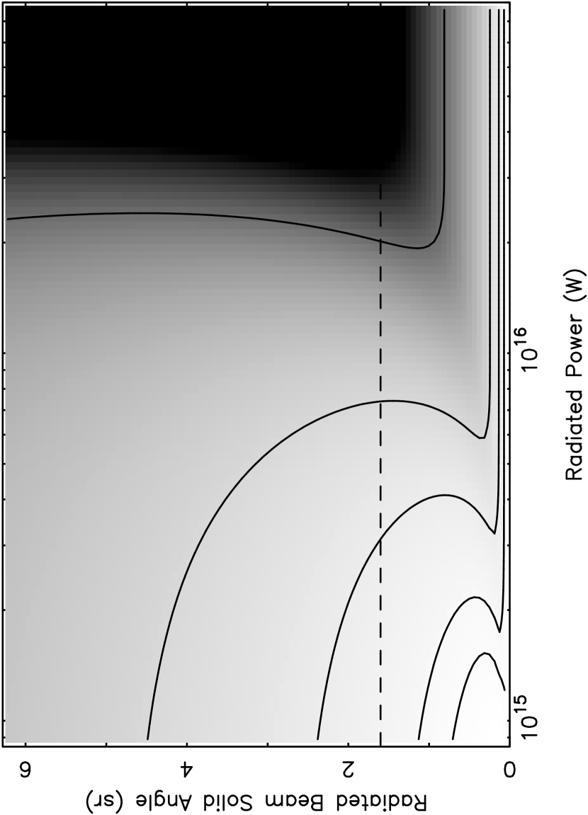
Figure 4: The (log-)likelihood function, equation 12, for detecting the radio emission from the planet orbiting $\tau$ Boo (catalog ) as a function of its radiated power $P_{\mathrm{rad}}$ and the solid angle $\Omega$ into which the radiation is beamed, assuming that it does radiate at a wavelength of 4 m. The gray scale is linear, with white indicating regions consistent with our non-detections and black indicating unlikely regions. The rms noise levels and flux densities used are listed in Tables 1 and 2; the bandwidth of the emission is assumed to be 37 MHz ($=74\,\mathrm{MHz}/2$). The maximum occurs in the lower left, near $P_{\mathrm{rad}}\simeq 10^{15}$ W and $\Omega\simeq 0.2$ sr; the first contour is at 99% of the peak, with subsequent contours at 98%, 95%, 90%, and 67%. The horizontal dotted line indicates the approximate beaming solid angle for Jupiter (catalog ) (Zarka & Cecconi, 2004).

Two comments on the likelihood function are warranted. First, the shape of the allowed region reflects two competing effects. From equation (3), the quantities $P_{\mathrm{rad}}$ and $\Omega$ are degenerate. The planet could radiate intensely but be beamed into a narrow solid angle, with a low probability of detection, or it could have a wide beaming angle but with only modest luminosity. The competing effect is that, as the beaming angle becomes smaller, the probability of it intersecting our line of sight becomes progressively smaller.

Second, the upper limit on $P_{\mathrm{rad}}$ in Figure 4 is motivated by predictions. A crucial element of the prediction by Stevens (2005) is that the stellar mass loss rate was predicted on the basis of the star’s X-ray flux. It now seems that stellar mass loss rates change character at a characteristic X-ray flux of about $8\times 10^{5}$ erg cm^-1 s^-1 (Wood et al., 2005). Below this value, stellar mass loss rates are highly correlated with X-ray flux; above this value, the mass loss rates drop by an order of magnitude and remain relatively constant with increasing X-ray fluxes. The X-ray flux of $\tau$ Boo (catalog ) is essentially equal to the value at which stellar mass loss rates change character. Thus, its mass loss rate could be overestimated by as much as an order of magnitude. Stevens (2005) predicts that the planet’s cyclotron maser strength should scale with the mass loss rate as $\dot{M}^{2/3}$. Thus, even if it is the case that the mass loss rate was overestimated by a factor of 10, the radiated power from the planet could still be a factor of 5 above that which would be estimated assuming a solar mass loss rate.

For our observations, assuming that the planet does radiate at a wavelength of 4 m, we conclude that the upper end of the predicted power levels is allowed only if the beaming angle is $\Omega\ll 1$ sr. The cyclotron maser emission from the solar system planets is characterized by solid angles $\Omega\gtrsim 1$ sr, typically emitted in a hollow cone, with a fairly wide opening angle ($\sim 90\arcdeg$) and a finite thickness. Recent analysis of Cassini observations of Jupiter (catalog ) during the spacecraft’s cruise phase indicate that its decameter radiation illuminates a cone of half-width opening angle of 75° and a thickness of 15°, with an equivalent solid angle $\Omega\simeq 1.6$ sr (Zarka & Cecconi, 2004). In some cases, for example the Earth’s auroral kilometric radiation, the beaming angle can be $\Omega\gtrsim\pi$ sr (Green & Gallagher, 1985).

For beaming angles comparable to those seen in the solar system ($\Omega\sim 1$ sr), the planet must radiate less than about $10^{16}$ W or we would have a reasonable probability of detecting it. Luminosities $P_{\mathrm{rad}}<10^{16}$ W are within the predicted range (Lazio et al., 2004; Stevens, 2005; Griessmeier et al., 2005), though below the most recent estimates that attempt to incorporate what is known about the star’s stellar wind strength. For comparison, Jupiter’s (catalog ) nominal radio luminosity is of order $10^{10}$ W.

Bastian et al. (2000) also subdivided each observation of a single star into scans as short as 10 s (the shortest nominal integration time provided by the VLA). The motivation is that Jupiter’s (catalog ) emission is quite variable, so, if the extrasolar planet radio emission is similar, subdividing the observation offers the possibility of detecting a “burst,” which might be quite short in duration and “diluted” if the entire ($\gtrsim 1$ hr) observation is considered. Though Bastian et al. (2000) did not observe $\tau$ Boo (catalog ) at 4-m wavelength, we have considered the impact of subdividing the observation. The obvious benefit of subdividing is that the effective number of observations increases; the disadvantage is that the noise level does as well.

We assume similar observing parameters as obtained in our observing programs, namely a point-source noise level $\sigma\approx 0.1$ Jy obtained in 1 hr for observations toward a star like $\tau$ Boo (catalog ). We find that sub-dividing the observation into 10 scans (e.g., each of 5 min. duration), which increases the noise level to $\sigma\approx 0.3$ Jy, leads to essentially no improvement in the constraints that can be set.

As a final comment on our likelihood method, we anticipate future observations, either with existing or future instruments (see below) might be at different wavelengths. A significant assumption in our likelihood analysis is that searches are conducted at a common wavelength and that the planet emits at that wavelength. In the case of Jupiter (catalog ), for instance, its electron cyclotron emission cuts off sharply shortward of approximately 7.5 meters ($\nu>40$ MHz). Presuming that similar processes operate in the magnetospheres of extrasolar giant planets, observations at different wavelengths may not be equally constraining. Similarly, one might wish to take into account what is known about the beaming angles from the solar system planets. It would be relatively straightforward to incorporate this prior information and extend our likelihood analysis to a Bayesian formulation. In that case, appropriate priors would have to be specified for the emission wavelength, beaming angle, and radiated power.

3.4 Future Observations

There are a number of next-generation, long wavelength radio instruments under development. Notable among these are the Low Frequency Array (LOFAR) and the Long Wavelength Array (LWA). If deployed as intended, both promise to provide sensitivities at least an order of magnitude larger than the 4-meter wavelength VLA at comparable wavelengths ($\lambda>3$ m or $\nu<100$ MHz). Here we consider whether additional observations with current instrumentation is preferable to the operation of these future facilities.

We simulated two sets of flux density measurements toward a star like $\tau$ Boo (catalog ). For both measurements the typical flux density measurement was taken to be a gaussian random variable with a specified mean and variance and the rms noise level was taken to be a factor of 2.5 times smaller. The first set of measurements had noise levels and flux density limits similar to those measured here, but we considered the impact of having 15 measurements rather than just 3. Not detecting planetary radio emission in such a data set would not improve significantly on the radiated power constraints (at most by a factor of a few) but would place increasingly severe constraints on the beaming angle at large power levels.

We have also considered the requirements on an instrument in order to improve the constraints significantly. Figure 5 illustrates the constraints placed by 5 measurements with an instrument capable of obtaining flux density measurements of approximately 25 mJy with rms noise levels of approximately 7 mJy beam^-1. Obtaining significant (an order of magnitude or better) improvements on the powers radiated by extrasolar planetary electron cyclotron masers will require measurements at this level. One significant advantage that future long-wavelength instruments are likely to have over current instruments, though, is that future instruments are likely to have a multi-beaming capability. Consequently, there is likely to be significantly more time for observation and a much larger number of measurements (or even detections!) will be obtained.

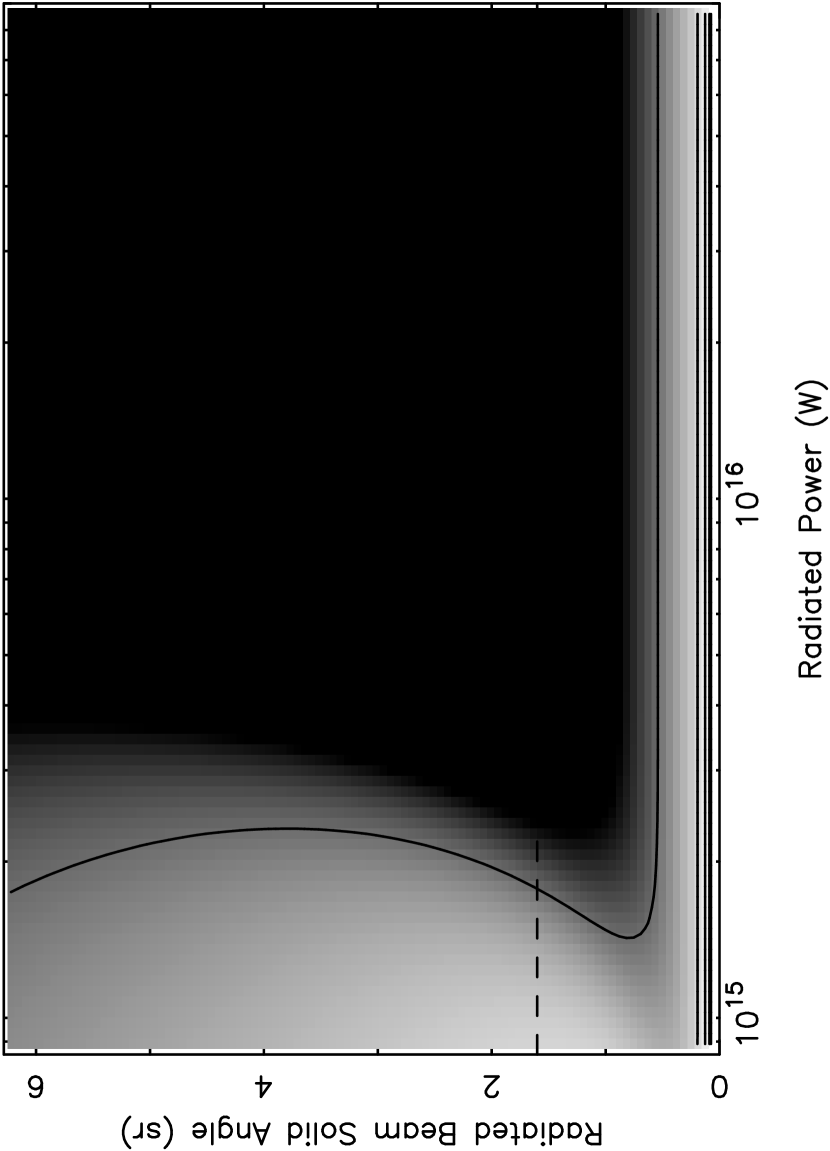
Figure 5: As for Figure 4, but for a next generation, long-wavelength instrument (e.g., the LWA or LOFAR) capable of flux density measurements in the range of 25 mJy with an rms noise level near 7 mJy beam^-1. In this case, five measurements were simulated.

4 Conclusions

We report three (3) epochs of 4-meter wavelength (74 MHz) observations of $\tau$ Boo (catalog ) with the VLA. Our objective was to detect the electron cyclotron maser emission from the planet orbiting this star, assuming that the planet does produce the equivalent of Jovian radio emissions. In none of our 3 epochs did we detect emission at the location of $\tau$ Boo (catalog ). For a single epoch (Table 2), our limits on its emission range from 150 to 300 mJy, equivalent to a range of luminosities of approximately 1–$2.5\times 10^{16}$ W. We have also stacked (“co-added”) the images to produce an average limit of 165 mJy, equivalent to a luminosity of $1.4\times 10^{16}$ W.

We have developed a likelihood method to consider multi-epoch measurements. Our likelihood function depends upon three planetary parameters, the planet’s radiated power level $P_{\mathrm{rad}}$, the beaming solid angle of the electron cyclotron maser $\Omega$, and the characteristic wavelength of emission $\lambda_{c}$. Under the assumption that the planet does radiate at our observed wavelength, the parameters $P_{\mathrm{rad}}$ and $\Omega$ are degenerate (Figure 4). We find that the typical radiated power must be less than about $10^{16}$ W unless the beaming solid angle is $\Omega\ll 1$ sr, which would be considerably smaller than the typical value for solar system planets. Power levels $P_{\mathrm{rad}}<10^{16}$ W are within the predicted range (Lazio et al., 2004; Stevens, 2005; Griessmeier et al., 2005), being comparable to or below the most recent estimates that attempt to incorporate what is known about the star’s stellar wind strength.

We have also considered future long-wavelength instruments, such as the LWA and LOFAR. We find that to improve significantly upon our constraints, future instruments will have to be able to measure typical flux densities of approximately 25 mJy.

References

- Bastian et al. (2000) Bastian, T. S., Dulk, G. A., & Leblanc, Y. 2000, ApJ, 545, 1058
- Butler et al. (1997) Butler, R. P., Marcy, G. W., Williams, E., Hauser, H., & Shirts, P. 1997, ApJ, 474, L115
- Catala et al. (2007) Catala, C., Donati, J.-F., Shkolnik, E., Bohlender, D., & Alecian, E. 2007, MNRAS, 374, L42
- Cohen et al. (2007) Cohen, A. S., Lane, W. M., Kassim, N. E., et al. 2007, AJ, in press
- Condon et al. (1998) Condon, J. J., Cotton, W. D., Greisen, E. W., Yin, Q. F., Perley, R. A., Taylor, G. B., & Broderick, J. J. 1998, AJ, 115, 1693
- Cornwell & Perley (1992) Cornwell, T. J. & Perley, R. A. 1992, A&A, 261, 353
- Farrell et al. (1999) Farrell, W. M., Desch, M. D., & Zarka, P. 1999, J. Geophys. Res., 104, 14025
- Farrell et al. (2003) Farrell, W. M., Desch, M. D., Lazio, T. J. W., Bastian, T., & Zarka, P. 2003, in Scientific Frontiers in Research on Extrasolar Planets, eds. D. Deming & S. Seager (ASP: San Francisco) p. 151
- Farrell et al. (2004) Farrell, W. M., Lazio, T. J. W., Desch, M. D., Bastian, T., & Zarka, P. 2004, in Bioastronomy 2002: Life Among the Stars, eds. R. Norris, C. Oliver, & F. Stootman (ASP: San Francisco) p. 73
- Green & Gallagher (1985) Green, J. L., & Gallagher, D. L. 1985, J. Geophys. Res., 90, 9641
- Griessmeier et al. (2005) Griessmeier, J.-M., Motschmann, U., Mann, G., & Rucker, H. O. 2005, “The Influence of Stellar Wind Conditions on the Detectability of Planetary Radio Emissions,” Astron. & Astrophys., 437, 717
- Lazio et al. (2004) Lazio, T. J. W., Farrell, W. M., Dietrick, J., Greenlees, E., Hogan, E., Jones, C., & Hennig, L. A. 2004, ApJ, 612, 511
- Majid et al. (2006) Majid, W., Winterhalter, D., Chandra, I., Kuiper, T., Lazio, J., Naudet, C., & Zarka, P. 2006, in Planetary Radio Emissions VI, eds. H. O. Rucker, W. S. Kurth, & G. Mann (Austrian Academy Science: Vienna) p. 589
- Perryman et al. (1997) Perryman, M. A. C., Lindegren, L., Kovalevsky, J., et al. 1997, A&A, 323, L49
- Ryabov et al. (2004) Ryabov, V. B., Zarka, P., Ryabov, B. P. 2004, Planet. Space Sci., 52, 1479–1491
- Shkolnik et al. (2005) Shkolnik, E., Walker, G. A. H., Bohlender, D. A., Gu, P.-G., & Kuerster, M. 2005, ApJ, 622, 1075
- Stevens (2005) Stevens, I. R. 2005, MNRAS, 356, 1053
- Winglee et al. (1986) Winglee, R. M., Dulk, G. A., & Bastian, T. S. 1986, ApJ, 309, L59
- Wood et al. (2005) Wood, B. E., Mueller, H.-R., Zank, G. P., Linsky, J. L., & Redfield, S. 2005, ApJ, 628, L143
- Worsley et al. (2005) Worsley, M. A., Fabian, A. C., Bauer, F. E., et al. 2005, MNRAS, 357, 1281
- Yantis et al. (1977) Yantis, W. F., Sullivan, W. T., III, & Erickson, W. C. 1977, Bull. Amer. Astron. Soc., 9, 453
- Zarka (2007) Zarka, P. 2007, Planet. Space Sci., in press
- Zarka (2006) Zarka, P. 2006, in Planetary Radio Emission VI, eds. H. O. Rucker et al. (Austrian Acad.: Vienna) p. 543
- Zarka & Cecconi (2004) Zarka, P., & Cecconi, B. 2004, J. Geophys. Res., 109, A09S15
- Zarka et al. (2001) Zarka, P., Treumann, R. A., Ryabov, B. P., & Ryabov, V. B. 2001, Ap&SS, 277, 293
- Zarka et al. (1997) Zarka, P., Queinnec, J., Ryabov, B. P., et al. 1997, in Planetary Radio Emission VI, eds. H. O. Rucker et al. (Austrian Acad.: Vienna) p. 101
- Zibetti et al. (2005) Zibetti, S., White, S. D. M., Schneider, D. P., & Brinkmann, J. 2005, MNRAS, 358, 949