Stochastic analysis and simulation of spin star systems

Abstract

We discuss two methods of an exact stochastic representation of the non-Markovian quantum dynamics of open systems. The first method employs a pair of stochastic product vectors in the total system’s state space, while the second method uses a pair of state vectors in the open system’s state space and a random operator acting on the state space of the environment. Both techniques lead to an exact solution of the von Neumann equation for the density matrix of the total system. Employing a spin star model describing a central spin coupled to bath of surrounding spins, we perform Monte Carlo simulations for both variants of the stochastic dynamics. In addition, we derive analytical expression for the expectation values of the stochastic dynamics to obtain the exact solution for the density matrix of the central spin.

I Introduction

The Markovian dynamics of an open quantum system $S$ which is coupled to an environment $E$ TheWork is conventionally described by a master equation for the open system’s density matrix $\rho_{S}(t)$ with a generator in Lindblad form GORINI ; LINDBLAD . It is a well-known feature DALIBARD ; DUM ; GISIN ; CARMICHAEL ; PLENIO of this type of master equations that it yields a stochastic representation for $\rho_{S}(t)$ in the form of an expectation value over an ensemble of pure state vectors. This means that $\rho_{S}(t)$ can be expressed by

$$\rho_{S}(t)={\mathrm{E}}(|\psi(t)\rangle\langle\psi(t)|),$$ (1)

where $|\psi(t)\rangle$ is a stochastic state vector in the Hilbert space of the open system and ${\mathrm{E}}$ denotes the expectation value. The great advantage of the stochastic representation consists in the fact that it leads to efficient Monte Carlo techniques in which one propagates an ensemble of pure state vectors in the open system’s Hilbert space and estimates the reduced density matrix through an appropriate ensemble average.

Recently, an exact stochastic treatment of non-Markovian quantum dynamics has been proposed PDP-PRA ; PDP-EPJD . This method is based on a representation of the density matrix $\rho(t)$ of the total system through an expectation value of the form

$$\rho(t)={\mathrm{E}}(|\Phi_{1}(t)\rangle\langle\Phi_{2}(t)|).$$ (2)

By contrast to the conventional approach one uses in this method a pair of random product vectors $|\Phi_{1}(t)\rangle=\psi_{1}(t)\otimes\chi_{1}(t)$ and $|\Phi_{2}(t)\rangle=\psi_{2}(t)\otimes\chi_{2}(t)$ of the total system. These product vectors follow independent stochastic time-evolution equations that can be constructed in such a way that the average over the probabilistic dynamics reproduces the exact Schrödinger or von Neumann dynamics of the total system. As demonstrated in PDP-PRA ; PDP-EPJD the evolution equations for the product vectors $|\Phi_{1}(t)\rangle$ and $|\Phi_{2}(t)\rangle$ can be chosen to be relatively simple time-local stochastic differential equations, describing a piecewise deterministic process or a diffusion process (Brownian motion) in Hilbert space. This means that it is possible to design a representation of non-Markovian quantum dynamics involving strong memory effects through a Markovian unravelling by means of a pair of independent stochastic product vectors.

This method bears several advantages. The stochastic differential equations for the product vectors describe a Markovian random process for which efficient numerical simulation algorithms are known (see, e. g., Ref. TheWork and references therein). Since the method is based on a direct stochastic representation of the full Schrödinger dynamics of the total system it does not rely on the construction of an approximate effective master equation for the reduced density matrix; it does not even require the existence of such an equation. Furthermore, the method allows, at least in principle, the treatment of arbitrary correlations in the initial state. This follows from the fact that any initial state $\rho(0)$ can be represented in the form $\rho(0)={\mathrm{E}}(|\Phi_{1}(0)\rangle\langle\Phi_{2}(0)|)$, where $|\Phi_{1}(0)\rangle$ and $|\Phi_{2}(0)\rangle$ are random product states PDP-EPJD . In particular, the method does not presuppose that system and environment are initially in an uncorrelated tensor product state. Finally, the technique not only allows the determination of the reduced density matrix $\rho_{S}(t)$ but also of multitime quantum correlation functions of the open system.

There is an important limitation in the applicability of the Monte Carlo algorithms based on the stochastic representation (2) which is due to the behavior of the statistical fluctuations. As shown in Ref. PDP-EPJD the fluctuations of the process and, hence, also the statistical errors of the Monte Carlo simulation may eventually grow exponentially with time. Therefore, the method can generally be expected to be feasible only for short time scales. However, it must be noted that the stochastic dynamics of the product vectors $|\Phi_{1}(t)\rangle$ and $|\Phi_{2}(t)\rangle$ is by no means unique, i. e., there exists an infinite number of stochastic evolution equations for which the expectation value (2) exactly represents the full system dynamics. Recently, this freedom in the choice of an appropriate stochastic dynamics has been employed to develop optimized Monte Carlo algorithms which lead to a drastic reduction of the size of statistical errors LACROIX .

The structure of Eq. (2) is not the only possibility of obtaining an exact stochastic representation for the total density matrix. In fact, one can construct many other random functionals whose expectation values lead to the desired equation of motion. Here, we examine an alternative stochastic formulation which employs a pair of random state vectors $|\psi_{1}(t)\rangle$ and $|\psi_{2}(t)\rangle$ in the open system’s Hilbert space and a random operator $R_{E}(t)$ on the state space of the environment:

$$\rho(t)={\mathrm{E}}(|\psi_{1}(t)\rangle\langle\psi_{2}(t)|\otimes R_{E}(t)).$$ (3)

Again, one can construct an appropriate stochastic dynamics for the state vectors $|\psi_{1}(t)\rangle$ and $|\psi_{2}(t)\rangle$ and for the environmental operator $R_{E}(t)$ that guarantees that the expectation value (3) exactly satisfies the von Neumann equation of the total system.

We start our considerations in Sec. II with a description of the general concepts underlying the stochastic representations given by Eqs. (2) and (3). The corresponding Monte Carlo simulation techniques will be illustrated in Sec. III with the help of a spin star model, i. e., a model of a central spin that is coupled to a bath of surrounding spins BBP . In addition to performing numerical simulations, we derive analytical expressions for the expectation values (2) and (3) and relate these directly to the solution of the Schrödinger equation for the total system. It turns out that the method described by Eq. (3) is particularly useful for the simulation of the dynamics for an infinite number of bath spins. Some conclusions are drawn in Sec. IV.

II Stochastic representations of non-Markovian quantum dynamics

II.1 General theory

We consider an open quantum system with Hilbert space ${\mathcal{H}}_{S}$ coupled to an environment with Hilbert space ${\mathcal{H}}_{E}$. The state space of the composite quantum system is given by the tensor product space ${\mathcal{H}}_{S}\otimes{\mathcal{H}}_{E}$. Employing the interaction picture we write the Hamiltonian describing the system-environment coupling as follows,

$$H_{I}(t)=\sum_{\alpha}A_{\alpha}(t)\otimes B_{\alpha}(t).$$ (4)

The $A_{\alpha}(t)$ and the $B_{\alpha}(t)$ are interaction picture operators acting in ${\mathcal{H}}_{S}$ and ${\mathcal{H}}_{E}$, respectively. The corresponding von Neumann equation for the density matrix $\rho(t)$ of the composite quantum system is given by

$$\frac{d}{dt}\rho(t)=-i[H_{I}(t),\rho(t)],$$ (5)

where we set $\hbar=1$.

Our aim is to construct a stochastic representation of the total density matrix $\rho(t)$ in terms of the expectation value

$$\rho(t)={\mathrm{E}}(R(t)).$$ (6)

Here, $R(t)$ represents a random operator on the state space ${\mathcal{H}}_{S}\otimes{\mathcal{H}}_{E}$ of the total system. The stochastic process governing the dynamics of this operator must be constructed in such a way that the expectation value (6) satisfies the von Neumann equation (5). It turns out that there are many possibilities of constructing a stochastic representation which meets this requirement. Of course, we do not seek just any stochastic formulation, but the intention is to find a stochastic process which leads to a considerable simplification of the representation of the reduced density matrix

$$\rho_{S}(t)={\mathrm{tr}}_{E}\rho(t)={\mathrm{E}}\left({\mathrm{tr}}_{E}R(t)\right)$$ (7)

of the open system and which allows an efficient numerical implementation of its time evolution (${\mathrm{tr}}_{E}$ denotes the partial trace over ${\mathcal{H}}_{E}$). In the following we discuss two (of many other) such possibilities, in which $R(t)$ follows a piecewise deterministic process (PDP) TheWork .

II.2 Stochastic process of the form $R=|\Phi_{1}\rangle\langle\Phi_{2}|$

The first possibility of a stochastic representation in terms of a PDP is given by taking $R(t)$ to be of the form

$$R(t)=|\Phi_{1}(t)\rangle\langle\Phi_{2}(t)|,$$ (8)

such that we have:

$$\rho(t)={\mathrm{E}}(|\Phi_{1}(t)\rangle\langle\Phi_{2}(t)|).$$ (9)

$|\Phi_{1}(t)\rangle$ and $|\Phi_{2}(t)\rangle$ represent a pair of stochastic state vectors of the composite quantum system which are chosen as direct products of system states $\psi_{\nu}(t)$ and environmental states $\chi_{\nu}(t)$:

$$|\Phi_{\nu}(t)\rangle=\psi_{\nu}(t)\otimes\chi_{\nu}(t),\qquad\nu=1,2.$$ (10)

In view of Eqs. (9) and (10) the reduced density matrix $\rho_{S}(t)$ [see Eq. (7)] can be expressed in terms of the expectation value:

$$\rho_{S}(t)={\mathrm{E}}\left(|\psi_{1}(t)\rangle\langle\psi_{2}(t)|\langle\chi_{2}(t)|\chi_{1}(t)\rangle\right).$$ (11)

By contrast to the standard stochastic unravelling of the dynamics of open quantum systems, this representation employs an average over the product of two quantities, namely the dyadic $|\psi_{1}\rangle\langle\psi_{2}|$ formed by a pair $\psi_{1}$, $\psi_{2}$ of state vectors of the open system, and the scalar product $\langle\chi_{2}|\chi_{1}\rangle$ of a corresponding pair of environment states.

According to the ansatz (10) the states $|\Phi_{\nu}(t)\rangle$ of the total system are direct products at any time $t$, which greatly simplifies the representation of the states of the system and the simulation of its dynamics. Of course, the exact states are generally entangled. This shows that the dynamics of the $|\Phi_{\nu}(t)\rangle$ cannot be described by a deterministic time evolution. However, as demonstrated in PDP-EPJD ; PDP-PRA it is possible to reproduce the dynamics of the total density matrix with the help of a random Markov process. An appropriate system of stochastic differential equations for the $\psi_{\nu}$ and the $\chi_{\nu}$ is given by

$$d\psi_{\nu}(t)=\sum_{\alpha}\left(\frac{-i||\psi_{\nu}||}{||A_{\alpha}(t)\psi_{\nu}||}A_{\alpha}(t)-I\right)\psi_{\nu}dN_{\alpha\nu}(t)$$ (12)

and

$$d\chi_{\nu}(t) = \Gamma_{\nu}(t)\chi_{\nu}dt$$

$$+ \sum_{\alpha}\left(\frac{||\chi_{\nu}||}{||B_{\alpha}(t)\chi_{\nu}||}B_{\alpha}(t)-I\right)\chi_{\nu}dN_{\alpha\nu}(t).$$

where $I$ denotes the unit operator. The quantities $dN_{\alpha\nu}$ are random Poisson increments which satisfy

$${\mathrm{E}}(dN_{\alpha\nu}(t))=\Gamma_{\alpha\nu}(t)dt$$ (14)

and

$$dN_{\alpha\nu}(t)dN_{\beta\mu}(t)=\delta_{\alpha\beta}\delta_{\nu\mu}dN_{\alpha\nu}(t).$$ (15)

The corresponding rates are given by

$$\Gamma_{\alpha\nu}(t)=\frac{||A_{\alpha}(t)\psi_{\nu}||\cdot||B_{\alpha}(t)\chi_{\nu}||}{||\psi_{\nu}||\cdot||\chi_{\nu}||},$$ (16)

and we have defined the total rates

$$\Gamma_{\nu}(t)\equiv\sum_{\alpha}\Gamma_{\alpha\nu}(t).$$ (17)

In view of Eq. (15) the stochastic increments $dN_{\alpha\nu}(t)$ take on the possible values $0$ or $1$. According to Eq. (14) the case $dN_{\alpha\nu}(t)=1$ occurs with probability $\Gamma_{\alpha\nu}dt$. Under the condition that $dN_{\alpha\nu}(t)=1$ for a particular $\alpha$ and $\nu$, the other increments vanish, and Eqs. (12) and (II.2) imply that for this particular $\alpha$ and $\nu$ the state vectors $\psi_{\nu}$ and $\chi_{\nu}$ perform the instantaneous jumps

$$\psi_{\nu}\rightarrow\frac{-i||\psi_{\nu}||}{||A_{\alpha}\psi_{\nu}||}A_{\alpha}\psi_{\nu},\qquad\chi_{\nu}\rightarrow\frac{||\chi_{\nu}||}{||B_{\alpha}\chi_{\nu}||}B_{\alpha}\chi_{\nu}.$$ (18)

Note that these jumps preserve the norm of the state vectors. Under the condition that all Poisson increments vanish, that is $dN_{\alpha\nu}(t)=0$ for all $\alpha$ and $\nu$, we have $d\psi_{\nu}(t)=0$ and $d\chi_{\nu}(t)=\Gamma_{\nu}\chi_{\nu}dt$. This means that $\psi_{\nu}$ remains unchanged during $dt$, while $\chi_{\nu}$ follows a linear drift.

Summarizing, $\psi_{\nu}(t)$ is a pure, norm-conserving jump process, whereas $\chi_{\nu}(t)$ is a PDP with norm-conserving jumps and a linear drift. It is demonstrated in PDP-EPJD that any initial density matrix of the total system can be represented in the form $\rho(0)={\mathrm{E}}(|\Phi_{1}(0)\rangle\langle\Phi_{2}(0)|)$, and that the expectation value (9) exactly satisfies the von Neumann equation (5). These facts enable us to simulate the full non-Markovian quantum dynamics through a Monte Carlo simulation of the stochastic differential equations (12) and (II.2).

II.3 Stochastic process of the form $R=|\psi_{1}\rangle\langle\psi_{2}|\otimes R_{E}$

The second possibility of a stochastic representation is obtained if we take $R(t)$ to be of the form

$$R(t)=|\psi_{1}(t)\rangle\langle\psi_{2}(t)|\otimes R_{E}(t),$$ (19)

such that we have:

$$\rho(t)={\mathrm{E}}(|\psi_{1}(t)\rangle\langle\psi_{2}(t)|\otimes R_{E}(t)).$$ (20)

In this case we represent $R(t)$ through a pair $\psi_{1}$, $\psi_{2}$ of state vectors of the open system and a random operator $R_{E}$ on the state space of the environment. The reduced density matrix of the open system can thus be written as

$$\rho_{S}(t)={\mathrm{E}}\left(|\psi_{1}(t)\rangle\langle\psi_{2}(t)|{\textrm{tr}}_{E}R_{E}(t)\right).$$ (21)

An appropriate system of stochastic differential equation which reproduces the exact von Neumann dynamics for the expectation value (20) is given by

$$d\psi_{\nu}(t) = \sum_{\alpha}\left(-iL_{\alpha\nu}A_{\alpha}-I\right)\psi_{\nu}(t)dN_{\alpha\nu}(t),$$ (22)

$$dR_{E}(t) = \Gamma R_{E}(t)dt$$ (23)

$$+\sum_{\alpha}\left(M_{\alpha 1}B_{\alpha}-I\right)R_{E}(t)dN_{\alpha 1}(t)$$

$$+\sum_{\alpha}R_{E}(t)\left(M_{\alpha 2}B^{\dagger}_{\alpha}-I\right)dN_{\alpha 2}(t).$$

The Poisson increments $dN_{\alpha\nu}$ satisfy Eqs. (14) and (15), and the transition rates are given by

$$\Gamma_{\alpha\nu}=\frac{1}{L_{\alpha\nu}M_{\alpha\nu}},$$ (24)

and

$$\Gamma_{\nu} = \sum_{\alpha}\Gamma_{\alpha\nu},$$ (25)

$$\Gamma = \Gamma_{1}+\Gamma_{2}.$$ (26)

The quantities $L_{\alpha\nu}$ and $M_{\alpha\nu}$ are real and positive functionals of $\psi_{1}$, $\psi_{2}$ and $R_{E}$. One has a great freedom in the choice of these functionals, the only restriction being the positivity. A definite choice will be made in the example below.

We observe that again the $\psi_{\nu}$ follow a pure jump process. If $dN_{\alpha\nu}(t)=1$ for a particular pair of indices $\alpha$ and $\nu$, which happens with probability $\Gamma_{\alpha\nu}dt$, the state vector $\psi_{\nu}$ undergoes the jump

$$\psi_{\nu}\rightarrow-iL_{\alpha\nu}A_{\alpha}\psi_{\nu}.$$ (27)

At the same time $R_{E}$ carries out the jump

$$R_{E}\rightarrow M_{\alpha 1}B_{\alpha}R_{E}$$ (28)

if $\nu=1$ and the jump

$$R_{E}\rightarrow R_{E}M_{\alpha 2}B^{\dagger}_{\alpha}$$ (29)

if $\nu=2$. Thus, for $\nu=1$ the operator $B_{\alpha}$ acts from the left on $R_{E}$, while for $\nu=2$ the adjoint operator $B^{\dagger}_{\alpha}$ acts from the right on $R_{E}$. Under the condition that all Poisson increments vanish, which occurs with probability

$$1-\sum_{\alpha\nu}\Gamma_{\alpha\nu}dt=1-\Gamma dt,$$ (30)

we have $d\psi_{\nu}(t)=0$ and $dR_{E}(t)=\Gamma R_{E}(t)dt$, i.e., the $\psi_{\nu}$ are left unchanged during $dt$ while the environment matrix $R_{E}(t)$ follows a linear drift.

Like in the case of the process constructed in Sec. II.2 it is easy to design an appropriate Monte Carlo algorithm for the stochastic differential equations (22) and (23). We note that in both cases the random matrix $R(t)$ has the structure of a tensor product, which considerably reduces the complexity of the problem. As a consequence of Eqs. (11) and (21) the environmental states enter the expectation value for the reduced density matrix $\rho_{S}(t)$ only through the scalar product $\langle\chi_{2}(t)|\chi_{1}(t)\rangle$ or through the trace ${\textrm{tr}}_{E}R_{E}(t)$. To simulate the non-Markovian dynamics of an open system with these algorithms it thus suffices to record during the simulation of the process the various jumps and their moments of occurrence. At any time $t$ the scalar product $\langle\chi_{2}(t)|\chi_{1}(t)\rangle$ or the trace ${\textrm{tr}}_{E}R_{E}(t)$ can then be expressed in terms of certain correlation functions of the environmental operators $B_{\alpha}$. For many system-environment models the latter are known explicitly. This fact greatly facilitates the numerical implementation of the stochastic method. An example is discussed in Sec. III.3 (see, in particular, Eq. (69)).

III Applications

III.1 The spin star model

As a simple but instructive example of the Monte Carlo method, we investigate in the following a spin star model described by the time independent interaction Hamiltonian

$$H=\frac{2A}{\sqrt{N}}\left(\sigma_{+}J_{-}+\sigma_{-}J_{+}\right).$$ (31)

The Pauli spin operator of the central spin, constituting the open system, is denoted by $\vec{\sigma}$ with corresponding raising and lowering operators $\sigma_{\pm}=\frac{1}{2}(\sigma_{1}\pm i\sigma_{2})$. The central spin couples to $N$ environment spins with Pauli spin operators $\vec{\sigma}^{(i)}$, $i=1,2,\ldots,N$, through the raising and lowering operators

$$J_{\pm}\equiv\sum^{N}_{i=1}\sigma^{(i)}_{\pm}=\frac{1}{2}\sum_{i=1}^{N}\left(\sigma^{(i)}_{1}\pm i\sigma^{(i)}_{2}\right)$$ (32)

of the total angular momentum $\vec{J}$ of the environment. The initial state of the total system at time $t=0$ is taken to be a product state $\rho(0)=\rho_{S}(0)\otimes\rho_{E}(0)$, where the reduced density matrix $\rho_{S}(0)$ of the central spin may be an arbitrary, possibly mixed state. The spin bath is assumed to be in an unpolarized infinite temperature initial state

$$\rho_{E}(0)=2^{-N}I_{E},$$ (33)

where $I_{E}$ denotes the unit matrix in ${\mathcal{H}}_{E}$.

This model can be solved analytically BBP . We express the solution for the reduced density matrix in terms of the components of the Bloch vector

$$\vec{v}(t)={\textrm{tr}}\left\{\sigma\rho(t)\right\}$$ (34)

which are related to the reduced density matrix by

$$\rho_{S}(t) = \left(\begin{array}[]{cc}\rho_{++}(t)&\rho_{+-}(t)\\ \rho_{-+}(t)&\rho_{--}(t)\end{array}\right)$$ (37)

$$= \frac{1}{2}\left(\begin{array}[]{cc}1+v_{3}(t)&v_{1}(t)-iv_{2}(t)\\ v_{1}(t)+iv_{2}(t)&1-v_{3}(t)\end{array}\right).$$ (40)

The components $v_{3}(t)$ and $v_{\pm}(t)\equiv\frac{1}{2}(v_{1}\pm iv_{2})$ are then given by the explicit expressions:

$$\!\!\!\!\!\!\!\!\!\frac{v_{3}(t)}{v_{3}(0)} = \sum_{j,m}P(j,m)\cos\left[2\Gamma(j,m)t\right],$$ (41)

$$\!\!\!\!\!\!\!\!\!\frac{v_{\pm(t)}}{v_{\pm}(0)} = \sum_{j,m}P(j,m)\cos\left[\Gamma(j,m)t\right]\cos\left[\Gamma(j,-m)t\right],$$ (42)

where

$$P(j,m)=\frac{1}{2^{N}}\left[\binom{N}{\frac{N}{2}+j}-\binom{N}{\frac{N}{2}+j+1}\right],$$ (43)

and

$$\Gamma(j,m)=2A\sqrt{\frac{j(j+1)-m(m+1)}{N}}.$$ (44)

These expressions may be obtained by solving the Schrödinger equation of the model with the help of the fact that the manifolds spanned by the states $|+\rangle\otimes|j,m\rangle$ and $|-\rangle\otimes|j,m+1\rangle$ are invariant under the time evolution. Here, $|\pm\rangle$ are the eigenstates of $\sigma_{3}$ with corresponding eigenvalues $\pm 1$, and $|j,m\rangle$ denotes an eigenstate of the square $\vec{J}\,^{2}$ of the angular momentum $\vec{J}$ of the spin bath and of its 3-component $J_{3}$ with respective eigenvalues $j(j+1)$ and $m$.

The quantity $P(j,m)$ defined in Eq. (43) is the probability of finding the quantum numbers $j$ and $m$ in the initial mixture representing the state (33) WESENBERG . As usual, for $N$ even $j$ takes on the values $j=0,1,2,\ldots,N/2$, and the values $j=1/2,3/2,\ldots,N/2$ if $N$ is odd. For a given $j$ the quantum number $m$ takes the values $-j,-j+1,\ldots,+j$. It is easy to check that the probability distribution $P(j,m)$ is normalized as follows,

$$\sum_{j,m}P(j,m)=1.$$ (45)

In the limit $N\rightarrow\infty$ of an infinite number of bath spins the above formulae lead to the asymptotic expressions BBP :

$$\frac{v_{3}(t)}{v_{3}(0)} = 1+2g(t),$$ (46)

$$\frac{v_{\pm(t)}}{v_{\pm}(0)} = 1+g(t),$$ (47)

where

$$g(t)\equiv-\frac{\sqrt{\pi}}{2}xe^{-x^{2}}\textrm{erfi}(x)=\sum^{\infty}_{k=1}\frac{(-1)^{k}k!}{2(2k)!}(2x)^{2k},$$ (48)

with $x\equiv\sqrt{2}At$. The function $\textrm{erfi}(x)$ denotes the imaginary error function, which is a real-valued function defined by

$$\textrm{erfi}(x)\equiv\frac{\textrm{erf}(ix)}{i}=\frac{2}{\sqrt{\pi}}\sum^{\infty}_{k=0}\frac{x^{2k+1}}{k!(2k+1)}.$$ (49)

III.2 The representation $R=|\Phi_{1}\rangle\langle\Phi_{2}|$

We first illustrate the stochastic representation for the process defined in Sec. II.2. To this end, the initial state (33) is realized through a mixture of the states $|j,m\rangle$, where the quantum numbers $j$ and $m$ follow the joint probability distribution $P(j,m)$ given in Eq. (43). To analyze the process we therefore have to describe the stochastic evolution of the initial states

$$|\Phi_{1}(0)\rangle=|\Phi_{2}(0)\rangle=|+\rangle\otimes|j,m\rangle,$$ (50)

or

$$|\Phi_{1}(0)\rangle=|\Phi_{2}(0)\rangle=|-\rangle\otimes|j,m\rangle,$$ (51)

from which we can reconstruct the reduced density matrix of the central spin.

Let us consider first the initial state (50). According to the interaction Hamiltonian (31) the index $\alpha$ in Eq. (4) assumes two values $\alpha=\pm$ with corresponding time independent operators

$$A_{\pm}=\sigma_{\pm},\qquad B_{\pm}=\frac{2A}{\sqrt{N}}J_{\mp}.$$ (52)

The jumps of the process thus take the form

$$\psi_{\nu}\rightarrow\frac{-i||\psi_{\nu}||}{||\sigma_{\pm}\psi_{\nu}||}\sigma_{\pm}\psi_{\nu},\qquad\chi_{\nu}\rightarrow\frac{||\chi_{\nu}||}{||J_{\mp}\chi_{\nu}||}J_{\mp}\chi_{\nu}.$$ (53)

Since $\psi_{\nu}(0)=|+\rangle$ the states $\psi_{\nu}$ jump between the states $|+\rangle$ and $|-\rangle$, whereby each jump contributes an additional factor of $(-i)$. Let us denote the number of jumps of $|\Phi_{\nu}\rangle$ during the time interval from $0$ to $t$ by $n_{\nu}=n_{\nu}(t)$. We then have $\psi_{\nu}(t)=(-i)^{n_{\nu}}|+\rangle$ if $n_{\nu}$ is even, and $\psi_{\nu}(t)=(-i)^{n_{\nu}}|-\rangle$ if $n_{\nu}$ is odd. The corresponding environment states are given by

$$\chi_{\nu}(t)=|j,m\rangle\,e^{\Gamma(j,m)t}$$ (54)

for even $n_{\nu}$, and by

$$\chi_{\nu}(t)=|j,m+1\rangle\,e^{\Gamma(j,m)t}$$ (55)

for odd $n_{\nu}$. The rates $\Gamma_{\pm}$ of the jumps are determined as follows,

$$\Gamma_{-} = \frac{2A}{\sqrt{N}}||J_{+}|j,m\rangle||=\Gamma(j,m),$$ (56)

$$\Gamma_{+} = \frac{2A}{\sqrt{N}}||J_{-}|j,m+1\rangle||=\Gamma(j,m).$$ (57)

Thus we have $\Gamma_{+}=\Gamma_{-}=\Gamma(j,m)$, where $\Gamma(j,m)$ is given by Eq. (44). The deterministic drift of the process therefore yields a factor $\exp[\Gamma(j,m)t]$, which has already been taken into account in Eqs. (54) and (55).

On using this information we can determine the dynamics of the populations of the reduced density matrix. Considering $\rho_{S}(0)=|+\rangle\langle+|$, we have by virtue of Eq. (11):

$$\rho_{++}(t) = \langle+|\rho_{S}(t)|+\rangle$$

$$= {\mathrm{E}}\left(\langle+|\psi_{1}(t)\rangle\langle\psi_{2}(t)|+\rangle\langle\chi_{2}(t)|\chi_{1}(t)\rangle\right)$$

$$= {\mathrm{E}}\left(w(n_{1},n_{2})(-i)^{n_{1}}(+i)^{n_{2}}e^{2\Gamma(j,m)t}\right).$$

Of course, a given realization of the process contributes to the expectation value only if $n_{1}$ and $n_{2}$ are even. This fact is accounted for by the first factor $w(n_{1},n_{2})$ which is defined to be equal to $1$ if $n_{1}$ and $n_{2}$ are even, and equal to zero otherwise. The second and the third factor under the expectation value take into account the jumps of $\psi_{1}$ (factor $(-i)^{n_{1}}$) and of $\psi_{2}$ (factor $\left[(-i)^{n_{2}}\right]^{\ast}=(+i)^{n_{2}}$). Finally, the exponential function represents the contributions from the scalar product $\langle\chi_{2}(t)|\chi_{1}(t)\rangle$ which, according to Eq. (54), equals $\exp[2\Gamma(j,m)t]$.

It is clear from the general theory outlined in Sec. II.2 that Eq. (III.2) is an exact representation of the populations. Nevertheless, it might be instructive to see explicitly how the exact solution (41) for the 3-component of the Bloch vector emerges from the expectation value (III.2). To this end, we note that the states $|\Phi_{\nu}\rangle$ evolve independently and that the transition rates of the process are time independent. This implies that the random numbers $n_{1}(t)$ and $n_{2}(t)$ follow independent Poisson distributions with the same mean value of $\Gamma(j,m)t$:

$$P(n_{\nu},t)=\frac{[\Gamma(j,m)t]^{n_{\nu}}}{n_{\nu}!}e^{-\Gamma(j,m)t}.$$ (59)

The expectation value (III.2) therefore becomes

$$\rho_{++}(t) = \sum_{j,m}P(j,m)\sum_{n_{1},n_{2}}(-i)^{n_{1}}(+i)^{n_{2}}$$ (60)

$$\qquad\times e^{2\Gamma(j,m)t}P(n_{1},t)P(n_{2},t).$$

The first sum extends over all possible values of the quantum numbers $j$ and $m$ occurring in the initial state (see Sec. III.1), while the second sum runs over all $n_{1},n_{2}=0,2,4,\ldots$. Substituting the expression (59) into Eq. (60), we get

$$\rho_{++}(t) = \sum_{j,m}P(j,m)\sum_{n_{1},n_{2}}(-i)^{n_{1}}(+i)^{n_{2}}$$ (61)

$$\qquad\times\frac{[\Gamma(j,m)t]^{n_{1}}}{n_{1}!}\frac{[\Gamma(j,m)t]^{n_{2}}}{n_{2}!}$$

$$= \sum_{j,m}P(j,m)\cos^{2}(\Gamma(j,m)t).$$

Using, finally, the relation $v_{3}(t)=2\rho_{++}-1$ we see that Eq. (61) leads to the exact expression (41) for the 3-component of the Bloch vector. Thus we see explicitly that the stochastic process indeed reproduces correctly the exact time evolution of the system.

In a similar way one finds the coherence $v_{-}(t)=\rho_{+-}(t)$ of the central spin. To this end, we have to consider also the initial state (51). The resulting process is essentially the same as above, with the only difference that now $\Gamma_{+}=\Gamma_{-}=\Gamma(j,-m)$. To find the expectation value representing $v_{-}(t)$ we have to use the initial states $|\Phi_{1}(0)\rangle=|+\rangle\otimes|j,m\rangle$ and $|\Phi_{2}(0)\rangle=|-\rangle\otimes|j,m\rangle$. With the initial condition $v_{-}(0)=1$ we then have

$$v_{-}(t) = \langle+|\rho_{S}(t)|-\rangle$$

$$= {\mathrm{E}}\left(\langle+|\psi_{1}(t)\rangle\langle\psi_{2}(t)|-\rangle\langle\chi_{2}(t)|\chi_{1}(t)\rangle\right)$$

$$= {\mathrm{E}}\left(w(n_{1},n_{2})(-i)^{n_{1}}(+i)^{n_{2}}e^{(\Gamma(j,m)+\Gamma(j,-m))t}\right).$$

It is easy to verify that this expectation value leads to the exact expression (42) for the coherence of the central spin.

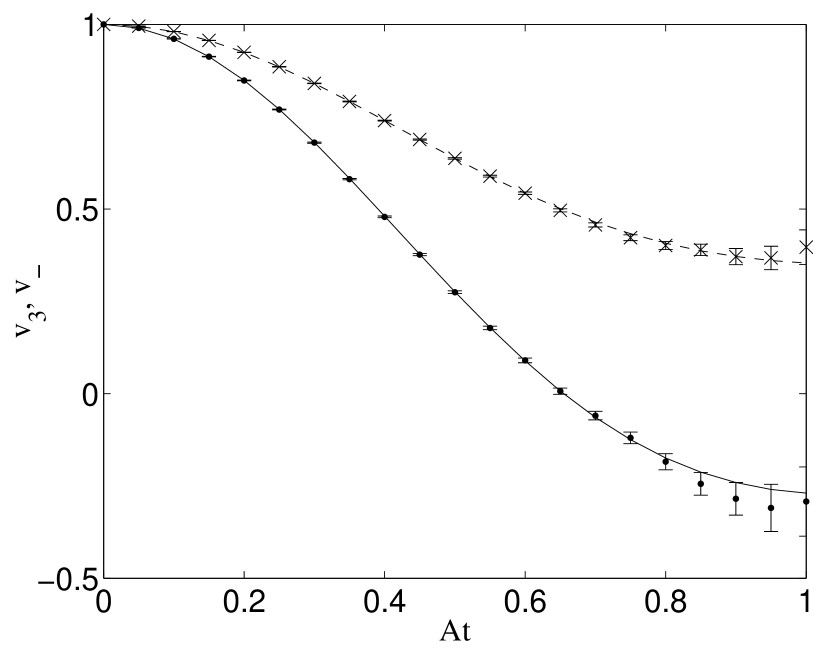
Figure 1: Monte Carlo simulation of Eqs. (12) and (II.2) using a sample of $10^{7}$ realizations: The 3-component $v_{3}=2\rho_{++}-1$ (dots and errorbars) of the Bloch vector and the coherence $v_{-}=\rho_{+-}$ (crosses and errorbars) of the central spin coupled to a bath of $10^{2}$ spins through the Hamiltonian (31). The continuous line and the broken line show the analytical solution given by Eqs. (41) and (42), respectively.

Figure 1 shows an example of a Monte Carlo simulation of the stochastic process defined by the differential equations (12) and (II.2). As can be seen, the Monte Carlo simulation reproduces the exact solution with high accuracy over the range of time shown. The figure also indicates the growth of the size of the statistical errors which have been estimated from the sample of realizations generated.

Beyond the point $At\approx 1$ the statistical errors strongly increase. This is a typical feature of the Monte Carlo simulation method which also appears in many other models. In fact, if one measures the size of the statistical errors by means of the Hilbert-Schmidt distance between the random operator $R(t)$ and its mean value $\rho(t)$, one can show PDP-EPJD that for large times the fluctuations grow roughly as $\exp(2\Gamma_{0}t)$, where $\Gamma_{0}$ represents an upper bound for the rates $\Gamma_{\nu}$. As can be seen from the above example this exponential increase of the errors is mainly due to the corresponding increase of the norm of the environmental states $\chi_{\nu}$.

III.3 The representation $R=|\psi_{1}\rangle\langle\psi_{2}|\otimes R_{E}$

Let us now analyze the process defined in Sec. II.3, which is particularly suited to simulate the limit of an infinite number $N$ of bath spins. We choose the quantities $L_{\alpha\nu}$ as follows:

$$L_{\alpha\nu}=\frac{||\psi_{\nu}||}{||A_{\alpha}\psi_{\nu}||}.$$ (63)

In our example we then have $L_{\alpha\nu}=1$. Thus, $\psi_{\nu}$ again jumps between states $|+\rangle$ and $|-\rangle$, whereby each jump contributes a factor of $(-i)$. Hence, we have

$$\rho_{++}(t)={\mathrm{E}}\left(w(n_{1},n_{2})(-i)^{n_{1}}(+i)^{n_{2}}{\textrm{tr}}_{E}R_{E}(t)\right).$$ (64)

The aim is now to determine the trace over the random environmental operator $R_{E}(t)$. This will be done in the limit $N\rightarrow\infty$. In this limit we have for a fixed number $k=0,1,2,\ldots$ BBP

$$\langle\left(J_{+}J_{-}\right)^{k}\rangle=k!\left(\frac{N}{2}\right)^{k},$$ (65)

where we define

$$\langle{\mathcal{O}}\rangle\equiv{\mathrm{tr}}_{E}\left\{{\mathcal{O}}\rho_{E}(0)\right\}=2^{-N}{\textrm{tr}}_{E}{\mathcal{O}}$$ (66)

for any bath operator ${\mathcal{O}}$. We further choose the jump rates $\Gamma_{1}=\Gamma_{2}=\sqrt{2}A$ (the factor $\sqrt{2}$ is introduced for convenience), such that $\Gamma=\Gamma_{1}+\Gamma_{2}=2\sqrt{2}A$. The drift contribution to $R_{E}(t)$ is therefore given by $\exp(2\sqrt{2}At)$. The jumps of the random matrix $R_{E}$ take the form

$$R_{E}\rightarrow\frac{1}{\sqrt{2}A}B_{\pm}R_{E}=\sqrt{\frac{2}{N}}J_{\mp}R_{E},$$ (67)

or

$$R_{E}\rightarrow\frac{1}{\sqrt{2}A}R_{E}B^{\dagger}_{\pm}=\sqrt{\frac{2}{N}}R_{E}J_{\pm}.$$ (68)

Since $R_{E}(0)$ is proportional to the identity and since the order of application of the operators $J_{\pm}$ is irrelevant in the limit $N\rightarrow\infty$, we conclude that

$${\textrm{tr}}_{E}R_{E}(t)=\left(\sqrt{\frac{2}{N}}\right)^{2k}\langle\left(J_{+}J_{-}\right)^{k}\rangle\,e^{\Gamma t},$$ (69)

where we have defined $k=(n_{1}+n_{2})/2$, assuming that both $n_{1}$ and $n_{2}$ are even. Employing Eq. (65) we therefore get

$${\textrm{tr}}_{E}R_{E}(t)=k!e^{\Gamma t}.$$ (70)

Hence, the expectation value (64) becomes:

$$\rho_{++}(t)={\mathrm{E}}\left(w(n_{1},n_{2})(-1)^{k}k!e^{\Gamma t}\right).$$ (71)

Figure 2: The 3-component $v_{3}=2\rho_{++}-1$ of the Bloch vector of the central spin coupled to an infinite number of bath spins through the Hamiltonian (31). Dots and errorbars: Monte Carlo simulation based on the stochastic differential equations (22) and (23) with $10^{7}$ realizations. Continuous line: Analytical solution given by Eqs. (46) and (48).

It is again instructive to see explicitly how this expression leads to the formulae (46) and (47). Using the fact that $n_{1}(t)$ and $n_{2}(t)$ are independent and follow Poisson distributions with mean value $\sqrt{2}At$, one finds

$$\rho_{++}(t) = \sum_{n_{1},n_{2}}\frac{(\sqrt{2}At)^{n_{1}}}{n_{1}!}\frac{(\sqrt{2}At)^{n_{2}}}{n_{2}!}(-1)^{k}k!$$

$$= \sum_{k=0}^{\infty}\frac{(-1)^{k}k!}{(2k)!}(\sqrt{2}At)^{2k}\sum_{n_{1}}\binom{2k}{n_{1}}.$$

We recall that the sum in the first line extends over the values $n_{1},n_{2}=0,2,4,\ldots$, and that we use the definition $k=(n_{1}+n_{2})/2$. The second sum in the second line runs over the values $n_{1}=0,2,\ldots,2k$. This sum is found to be equal to $1$ for $k=0$ and equal to $2^{2k-1}$ for $k=1,2,3,\ldots$. Thus we obtain

$$\rho_{++}(t)=1+\sum_{k=1}^{\infty}\frac{(-1)^{k}k!}{2(2k)!}(2\sqrt{2}At)^{2k}\equiv 1+g(t),$$ (72)

from which we get $v_{3}(t)=2\rho_{++}(t)-1=1+2g(t)$, where the function $g(t)$ has been introduced in Eq. (48). A similar reasoning leads to the relation $v_{\pm}(t)=1+g(t)$. These results coincide with those obtained from the solution of the Schrödinger equation [see Sec. III.1].

Figure 2 shows the results of a Monte Carlo simulation of the stochastic process defined by the differential equations (22) and (23). The Monte Carlo simulation reproduces the exact solution with high accuracy over the range of time shown, and we again observe the growth of the statistical errors.

IV Conclusions

We have investigated two methods that yield an exact stochastic unravelling of the non-Markovian quantum dynamics of open systems by means of a piecewise deterministic Markov process. These methods yield Monte Carlo simulation techniques that are generally applicable for the investigation of the short-time behavior of the open system’s dynamics. Due to a possible exponential increase of statistical fluctuations for large times a numerical simulation of the long time behavior is, in general, impossible in practice.

However, a great advantage of the method is given by the fact that it is exact and that it allows the treatment of arbitrary correlations in the initial state. It must be emphasized that a Monte Carlo simulation not only yields an estimate for the desired averages, but also for the statistical errors. As long as the latter are small the technique yields excellent predictions about the short-time behavior and thus offers the possibility to control and assess the performance of other approaches and approximation schemes. In particular, the method may find important applications in the simulation of non-Markovian decoherence phenomena which are dominated by the short time behavior of the open system.

The formulation of the stochastic simulation method has been given here in the interaction picture, assuming that the free dynamics of the system and the environment are known. If this is not the case one can use an analogous formulation of the stochastic dynamics in the Schrödinger picture which includes the given Hamiltonian operators for the system and the environment into the deterministic drift of the stochastic differential equations PDP-EPJD .

In our examples we have restricted ourselves to the case of an unpolarized (infinite temperature) initial state of the spin bath. It should be noted that the stochastic method is also applicable to polarized initial states. For instance, one can consider an initial equilibrium state of finite temperature. Introducing a spin bath Hamiltonian of the form $H_{E}=\omega J_{3}$, one then has to multiply the probability distribution $P(j,m)$ defined in Eq. (43) with the $m$-dependent Boltzmann factor $\exp(-\beta\omega m)$, where $\beta$ is the inverse temperature.

There are two basic strategies for the improvement of the Monte Carlo technique. The first one employs the freedom in the choice of the stochastic time-evolution in order to minimize the statistical errors LACROIX ; SHAO . This can be done by an appropriate modification of the noise terms of the stochastic differential equations. A further possibility is to introduce additional terms in the deterministic part of the equations of motion. This approach leads to a stochastic mean field dynamics which is similar to the one used in the Monte Carlo wave function method for interacting many-body systems CARUSO .

The second strategy is to reduce the size of the statistical fluctuations by using more complicated stochastic functionals whose expectation values lead to the reduced density matrix. The methods investigated here represent the correlated states of the composite system through the average over random operators with a specific given structure, namely a tensor product structure. This ansatz does by no means exhaust all possibilities. There are many other possible ways of constructing an exact stochastic representation of the dynamics which seem worth being explored in a more systematic manner.

- (1) H. P. Breuer and F. Petruccione, The Theory of Open Quantum Systems (Oxford University Press, Oxford, 2007).
- (2) V. Gorini, A. Kossakowski, and E. C. G. Sudarshan, J. Math. Phys. 17, 821 (1976).
- (3) G. Lindblad, Commun. Math. Phys. 48, 119 (1976).
- (4) J. Dalibard, Y. Castin, and K. Mølmer, Phys. Rev. Lett. 68, 580 (1992).
- (5) R. Dum, P. Zoller, and H. Ritsch, Phys. Rev. A 45, 4879 (1992).
- (6) N. Gisin and I. C. Percival, J. Math. Phys. A: Math. Gen. 25, 5677 (1992).
- (7) H. Carmichael, An Open Systems Approach to Quantum Optics, Lecture Notes in Physics m18 (Springer-Verlag, Berlin, 1993).
- (8) M. B. Plenio and P. L. Knight, Rev. Mod. Phys. 70, 101 (1998).
- (9) H. P. Breuer, Eur. Phys. J. D 29, 105 (2004).
- (10) H. P. Breuer, Phys. Rev. A 69, 022115 (2004).
- (11) D. Lacroix, Phys. Rev. A 72, 013805 (2005).
- (12) H. P. Breuer, D. Burgarth, and F. Petruccione, Phys. Rev. B 70, 045323 (2004).
- (13) J. Wesenberg, K. Mølmer, Phys. Rev. A 65, 062304 (2002).
- (14) Y. Zhou, Y. Yan, and J. Shao, Europhys. Lett. 72, 334 (2005).
- (15) I. Carusotto, Y. Castin, and J. Dalibard, Phys. Rev. A 63, 023606 (2001).