Magnetic reconnection at the termination shock in a striped pulsar wind.

Abstract

Context. Most of the rotational luminosity of a pulsar is carried away by a relativistic magnetised wind in which the matter energy flux is negligible compared to the Poynting flux. However, observations of the Crab nebula for instance clearly indicate that most of the Poynting flux is eventually converted into ultra-relativistic particles. The mechanism responsible for transformation of the electro-magnetic energy into the particle energy remains poorly understood. Near the equatorial plane of an obliquely rotating pulsar magnetosphere, the magnetic field reverses polarity with the pulsar period, forming a wind with oppositely directed field lines. This structure is called a striped wind; dissipation of alternating fields in the striped wind is the object of our study.

Aims. The aim of this paper is to study the conditions required for magnetic energy release at the termination shock of the striped pulsar wind. Magnetic reconnection is considered via analytical methods and 1D relativistic PIC simulations.

Methods. An analytical condition on the upstream parameters for partial and full magnetic reconnection is derived from the conservation laws of energy, momentum and particle number density across the relativistic shock. Furthermore, by using a 1D relativistic PIC code, we study in detail the reconnection process at the termination shock for different upstream Lorentz factors and magnetisations.

Results. We found a very simple criterion for dissipation of alternating fields at the termination shock, depending on the upstream parameters of the flow, namely, the magnetisation $\sigma$, the Larmor radius $r_{\rm B}$ and the wavelength $l$ of the striped wind. The model depends also on a free parameter $\xi>1$, which is the ratio of the current sheet width to the particle Larmor radius. It is found that for $\sigma\gg l/\xi\,r_{\rm B}$, all the Poynting flux is converted into particle energy whereas for $\sigma\ll(l/\xi\,r_{\rm B})^{2/3}$, no dissipation occurs. In the latter case, the shock can be accurately described by the ideal MHD shock conditions. Finally, 1D relativistic PIC simulations confirm this prediction and enable us to fix the free parameter $\xi$ in the analytical model.

Conclusions. Alternating magnetic fields annihilate easily at relativistic highly magnetised shocks. In plerions, our condition for full magnetic dissipation is satisfied at the termination shock so that the Poynting flux may be converted into ultra-relativistic particles not in the pulsar wind but just at the termination shock. The constraints are more severe for the intra-binary shocks in double pulsar systems. Available models explaining observations require low magnetisation in the downstream flow. The condition that the magnetic field dissipates at the intra-binary shock implies an upper limit on the pair multiplicity in the pulsar wind $\kappa$. We found $\kappa\lesssim{\rm few}\times 10^{4}$ for PSR 1259-63 and PSR 1957+20. In the double pulsar PSR 0737-3039, the radio emission from the pulsar B is modulated with the period of the pulsar A, which implies that the striped structure is not erased completely; this gives a lower limit for $\kappa\gtrsim 310$.

1 INTRODUCTION

Relativistic shock fronts and currents sheets in relativistic flows play an important role in astrophysical models of gamma-ray bursts, for a review see Piran (2005), jets in active galactic nuclei and pulsar winds, see for instance Michel (2005) and Kirk (2005). The underlying plasma is probably composed of electrons, positrons and/or protons, whose temperature may be relativistic, i.e. comparable or larger than their rest mass energy. A shock front is created whenever a fast flow encounters the interstellar or intergalactic medium. Relativistic effects become important when the post shock temperature is so high that the speed of particles approaches the speed of light $c$ or when the bulk velocity of the flow is close to $c$. Shock acceleration is used to explain the observed radiation from gamma-ray bursts or active galactic nuclei. In this paper, we focus on relativistic shocks arising form the interaction of the pulsar wind with its surrounding medium. For a detailed review on theoretical aspects on pulsar wind and plerions, see Lyubarsky (2005a). We briefly recall the main issue in this introduction.

It is widely assumed that most of the rotational energy of a pulsar is carried away in the form of an ultra-relativistic magnetised wind. The outflow is dominated by the magnetic field in the sense that the energy carried away by the plasma remains small compared to the Poynting flux. This is usually described by the magnetization parameter $\sigma$, the ratio of the Poynting flux to the particle energy flux, which is very large, $\sigma\gg 1$. Therefore the total power lost by the pulsar may be conveniently estimated by the loss rate of the rotating magnetic dipole in vacuum, (Michel, 1991). In the general case of an oblique rotator, energy loss can be thought as being shared between the steady axisymmetric component and one oscillating with the period of the pulsar, the ratio being determined by the angle between the rotational and the magnetic axes. Michel (1971) pointed out that such waves, which have a phase speed less than that of light, should evolve into regions of cold magnetically dominated plasma separated by narrow hot current sheets. This structure is called a striped pulsar wind and has originally been introduced by Coroniti (1990) and Michel (1994).

The structure of this striped wind can be explained as follows. In the aligned rotator, a radially outflowing stream of particles opens up the dipolar magnetic field lines crossing the light cylinder. Asymptotically, the stream lines become radial and can be described by the so-called split monopole solution (Michel, 1973). It consists of two half magnetic monopoles with equal magnitude but opposite sign separated by the equatorial plane. When crossing this equatorial plane, the polarity of the magnetic field reverses, implying a surface current density, i.e. the current sheet. If the rotation axis is tilted with respect to the magnetic moment, the current sheet oscillates around the equatorial plane and develops a wave structure, expanding radially at a speed close to the light velocity. In a radial outflow, the amplitude of the oscillations grows linearly with radius and at large distances can be approximated locally by spherical current sheets separating the stripes of magnetised plasma with opposite magnetic polarity. The exact solution for the oblique split monopole in the ideal MHD approximation has been found by Bogovalov (1999). Simulations by Spitkovsky (2006) in the force-free limit show that beyond the light cylinder, the wind from an oblique dipole pulsar magnetosphere is similar to that from the split monopole. The structure of the current sheet in the striped wind is shown in Fig. 1. Note that the oscillating current sheet is found in the solar wind so that this structure is generic.

Figure 1: Structure of the current sheet in the oblique rotator. The rotating neutron star is located at the centre. When crossing the current sheet, the magnetic polarity is reversed. Moreover, this structure is expanding radially outwards with a constant speed close to the light velocity.

While expanding into the nebula, the pulsar wind terminates at a standing shock located at a distance where the confining pressure of the nebula balances the ram pressure of the wind, this is called the termination shock, (Rees & Gunn, 1974; Kennel & Coroniti, 1984a, b; Emmering & Chevalier, 1987). At the shock front, the energy in the wind is released into ultra-relativistic particles responsible for the observed radiation. Observations of the interaction between the wind and the neighboring nebula clearly indicate that the electromagnetic energy of the wind is largely converted into particle kinetic energy. However, the conversion mechanism and the corresponding acceleration process still remain unclear.

Indeed, the analysis done by different authors, (Tomimatsu, 1994; Beskin et al., 1998; Chiueh et al., 1998; Bogovalov & Tsinganos, 1999; Lyubarsky & Eichler, 2001) shows that in an ultra-relativistic, radial wind, the electric force compensates the magnetic tension so that the flow could not be accelerated significantly. This means that the electromagnetic energy is not transferred to the plasma. To sum up, in the region where the wind is launched, the magnetisation should be high, $\sigma\gg 1$, whereas just beyond the termination shock, it should be small, $\sigma\ll 1$. But according to the previous results on MHD wind collimation and acceleration, a significant decrease in $\sigma$ is forbidden. Therefore, there is a contradiction which is known as the $\sigma$-problem. A promising alternative solution to convert the Poynting flux to particle kinetic energy is investigated in this paper. We demonstrate that, under certain conditions, magnetic reconnection in the striped wind occurs when it crosses the termination shock.

Both observations of the inner region of the Crab nebula done by Weisskopf et al. (2000) and the solution by Bogovalov (1999) show that most of the energy carried by the wind is transported in the equatorial plane of the pulsar wind. In this region, energy is transferred predominantly by the alternating magnetic field. So dissipation of alternating fields in the striped wind could be the main energy conversion mechanism in pulsars. It was recognised by Usov (1975) and Michel (1982) that the amplitude of the magnetic oscillations decreases with the distance as $r^{-1}$ whereas the particle number density sustaining these waves falls off as $r^{-2}$ where $r$ is the radius in spherical coordinates. At a given point, the charge carriers become insufficient to maintain the required current and the alternating field annihilates. Coroniti (1990) considered magnetic reconnection in the striped wind and was lead to the same conclusion. However, the flow is accelerated during the process of magnetic dissipation, which dilates the timescale of the wave decay such that the magnetisation remains high at the termination shock, (Lyubarsky & Kirk, 2001). Therefore, the wind enters the termination shock still dominated by Poynting flux unless the annihilation rate is nearly to the causal limit, (Kirk & Skjæraasen, 2003). However, when the flow enters the shock, the plasma is compressed, which could result in the forced annihilation of the alternating magnetic fields. In this paper, we address annihilation of alternating fields at a relativistic shock in electron-positron plasma.

In Lyubarsky (2003), the reconnection of the magnetic field at the termination shock was studied phenomenologically by introducing a fraction $\eta$ of the magnetic energy dissipated at the shock. Relativistic MHD shock fronts with dissipation have already been studied by Levinson & van Putten (1997). The jump conditions for a relativistic perpendicular ideal MHD shock with arbitrary magnetisation has been investigated by Zhang & Kobayashi (2005) in the context of GRBs. In the present paper, we use a kinetic description of the plasma in the striped wind. First we find jump conditions assuming that the thickness of the current sheets downstream of the shock is scaled as the particle Larmor radius; this gives us the fraction of the dissipated magnetic energy as a function of upstream parameters and of a phenomenological parameter, $\xi>1$, which is defined as the ratio of the sheet width to the Larmor radius. Then we perform particle-in-cell (PIC) simulations of the shock in the striped wind (such simulations were shortly described in Lyubarsky (2005b)) and find the parameter $\xi$ from the simulation results. We show that the alternating fields are easily annihilated at the shock front so that the electromagnetic energy of the pulsar wind could be readily converted into the plasma energy at the termination shock. This could provide a solution to the $\sigma$-problem.

The paper is organised as follows. In Sect. 2, we present the full system for the jump conditions of the averaged quantities in the striped wind. In Sect.3, we solve the system analytically. We derive an analytical condition for magnetic annihilation for an ultra-relativistic and strongly magnetised flow. The results are then checked and extended by numerically solving the jump conditions at the termination shock for the average parameters. In Sect.4, we perform several 1D PIC simulations of the striped wind by varying the parameters in the upstream plasma like the Lorentz factor and the magnetisation. Two typical situations are presented, the first one demonstrating that no magnetic energy is released at all and the second one showing full dissipation of the Poynting flux which is converted into particle heating. An empirical law for dissipation is then derived from the full set of PIC simulations. The results are compared to those obtained in Sect. 3. In Sect.5, the results are applied to pulsars in binary systems. On one hand, magnetic dissipation at the termination shock implies an upper limit on the pair multiplicity factor $\kappa$. Applications are presented for two binary pulsars, PSR 1259-63 and PSR 1957+20. On the other hand, an absence of significant dissipation imposes a lower limit on $\kappa$. This is applied to the double pulsar PSR 0737-3039. The conclusion are presented in Sect. 6.

2 JUMP CONDITIONS IN THE SHOCK

In this section, we derive the criterion for dissipation of alternating field at the shock by considering the jump conditions for the averaged quantities in the flow, namely, the conservation of the energy, momentum and the particle number density. We assume that the striped structure survives in the downstream flow and find the condition of the total dissipation of the alternating fields from the condition that the thickness of the current sheet downstream of the shock approaches the thickness of the stripes.

2.1 Description of the wind flow

Let us consider a one dimensional striped pulsar wind entering the termination shock. By convention, we refer to quantities in the shock frame with unprimed letters, while in the proper frame of each plasma, quantities are denoted by a prime. However, thermodynamical quantities such as pressure $p$, temperature $T$, internal energy $e$ and enthalpy $w$, are always expressed in the proper frame, so dropping primes should not lead to any confusion for these quantities.

The striped wind propagates in the $x$-direction with relativistic velocity and possesses an alternating magnetic field directed along the $z$-axis. Moreover, in this and the next sections we assume that its average over one period of the striped wind vanishes. Quantities upstream, i.e. before crossing the shock discontinuity are subscripted by 1 whereas quantities downstream are subscripted by 2.

Let us describe the state of the incoming plasma. In the shock frame, the upstream Lorentz factor of the ultra-relativistic wind is $\Gamma_{1}\gg 1$. The current sheets are made of a hot, unmagnetised plasma with density $n_{\rm h1}$ and a temperature $T_{\rm h1}$. The distance separating the middle of two successive current sheets is denoted by $l_{1}$ (half a wavelength of the wind) and their thickness $\Delta_{1}$ is much less than half a wavelength, $\Delta_{1}\ll l_{1}$. The magnetised part of the wind is cold, $T_{\rm c1}=0$, has a density $n_{\rm c1}$ and a magnetic field strength $B_{1}$. Moreover, the wind is strongly magnetised such that the magnetisation parameter upstream defined by

$$\sigma_{1}=\frac{B_{1}^{2}}{\mu_{0}\,\Gamma_{1}^{2}\,w_{\rm c1}}=\frac{B_{1}^{2}}{\mu_{0}\,\Gamma_{1}\,n_{\rm c1}\,m\,c^{2}}$$ (1)

is very high, $\sigma_{1}\gg 1$. The enthalpy is simply given by the rest mass energy of the cold ultra-relativistic particles, $w_{\rm c1}=n_{\rm c1}^{\prime}\,m\,c^{2}$. The speed of light is $c$ and $m$ is the mass of the leptons composing the wind, actually electrons and positrons. We neglect the enthalpy contribution from the hot current sheets because their thickness is assumed to be very small.

Downstream, the wind is decelerated to a Lorentz factor $\Gamma_{2}$ and compressed such that the distance separating two successive current sheets shrinks to a length $l_{2}$. When compressed, the cold magnetised component of the wind is heated to a temperature $T$ given in the limit of high magnetisation, $\sigma_{1}\gg 1$, and high Lorentz factor, $\Gamma_{1}\gg 1$, by (Kennel & Coroniti, 1984a) (see also appendix A) :

$$\frac{k_{B}\,T}{m\,c^{2}}=\frac{1}{8}\,\frac{\Gamma_{1}}{\Gamma_{2}}$$ (2)

$k_{B}$ is the Boltzmann constant. We assume here that the shock width is much less than the wavelength of the wind. When the shock is between the sheets, ideal MHD shock applies and Eq. (2) is locally valid. Note also that the shock velocity in the cold part is close to the speed of light $c$ and different from the shock velocity in the hot part. Quantities are evaluated in the frame where the shock is at rest on average. Eq. (2) is valid in any frame.

Note that even if the upstream flow is a pure entropy wave with a constant magnetic field between the sheets, fast magnetosonic waves should be generated beyond the shock. Therefore the structure downstream is not steady in the proper frame; there should be oscillations. We consider quantities averaged over the wave period and neglect contribution of these oscillations into the fluxes.

Pressure balance between gaseous and magnetic part does therefore apply on both sides of the discontinuity. The gaseous pressures are given by :

$$p_{1} = n_{\rm h1}^{\prime}\,k_{B}\,T_{\rm h1}$$ (3)

$$p_{2} = n_{\rm h2}^{\prime}\,k_{B}\,T_{\rm h2}$$ (4)

$$p_{\rm c2} = n_{\rm c2}^{\prime}\,k_{B}\,T=\frac{1}{8}\,\frac{\Gamma_{1}}{\Gamma_{2}}\,n_{\rm c2}^{\prime}\,m\,c^{2}$$ (5)

Note that the “cold” part of the wind is heated to relativistic temperature downstream and therefore also contributes to the gaseous pressure via the term $p_{\rm c2}$, where the temperature is given according to Eq. (2). In other words, upstream we have

$$p_{1}=\frac{B_{1}^{2}}{2\,\mu_{0}\,\Gamma_{1}^{2}}$$ (6)

whereas downstream, taking into account the heated cold component, we find

$$p_{2}=p_{c2}+\frac{B_{2}^{2}}{2\,\mu_{0}\,\Gamma_{2}^{2}}$$ (7)

Due to the Lorentz length contraction, the densities in the proper frame and in the shock frame are related by $n=\Gamma\,n^{\prime}$. On the other hand, the Lorentz transformation of the magnetic field is $B=\Gamma\,B^{\prime}$.

2.2 Jump conditions for average quantities

We now write down the MHD jump conditions for the quantities averaged over one wavelength of the wind. Following the procedure described in Lyubarsky (2003) for a perpendicular MHD shock, the conservation laws can be cast in a form similar to those for a relativistic hydrodynamical flow. Noting that in the cold magnetised part, the field is frozen into the plasma

$$\frac{B_{1}}{\Gamma_{1}\,n^{\prime}_{c1}}=\frac{B_{2}}{\Gamma_{2}\,n^{\prime}_{c2}}\equiv\frac{B_{1}}{n_{c1}}=\frac{B_{c2}}{n_{c2}}$$ (8)

such that the magnetic field becomes a function of the density, one can introduce the effective pressure and enthalpy by :

$$\mathcal{P}_{i} = p_{i}+\frac{B_{i}^{2}}{2\,\mu_{0}\,\Gamma_{i}^{2}}$$ (9)

$$\mathcal{W}_{i} = w_{i}+\frac{B_{i}^{2}}{\mu_{0}\,\Gamma_{i}^{2}}$$ (10)

Now the jump conditions at the shock discontinuity are given by

• conservation of particle number density :

  $$\langle\Gamma_{1}\,\beta_{1}\,n_{1}^{\prime}\rangle=\langle\Gamma_{2}\,\beta_{2}\,n_{2}^{\prime}\rangle\equiv\langle\beta_{1}\,n_{1}\rangle=\langle\beta_{2}\,n_{2}\rangle;$$ (11)

• conservation of total energy :

  $$\langle\Gamma_{1}^{2}\,\beta_{1}\,\mathcal{W}_{1}\rangle=\langle\Gamma_{2}^{2}\,\beta_{2}\,\mathcal{W}_{2}\rangle;$$ (12)

• conservation of total momentum :

  $$\langle\Gamma_{1}^{2}\,\beta_{1}^{2}\,\mathcal{W}_{1}+\mathcal{P}_{1}\rangle=\langle\Gamma_{2}^{2}\,\beta_{2}^{2}\,\mathcal{W}_{2}+\mathcal{P}_{2}\rangle.$$ (13)

Here $\beta_{1,2}c$ are the upstream and downstream velocities, correspondingly and the angular brackets, $\langle\rangle$, mean averaging over the wave period, which means spatial averages. We assume that the downstream flow is settled into an equilibrium pattern moving with constant velocity, i.e. that only an entropy wave is presented downstream. Then time averages are expressed via spatial averages; e.g. the average particle flux is

$$\frac{1}{T}\,\int_{0}^{T}n\,\beta\,dt=\frac{1}{T}\,\int_{0}^{l}n\,dx=\frac{\beta}{l}\,\int_{0}^{l}n\,dx.$$ (14)

As the time-averaged particle flux (the left-hand side of Eq. (14)) is constant and the total number of particles within the wavelength ($\int_{0}^{l}n\,dx$) is conserved, Eq. (14) yields a useful relation between the upstream and downstream wavelengths:

$$\frac{\beta_{1}}{l_{1}}=\frac{\beta_{2}}{l_{2}}.$$ (15)

Of course, our assumption is not exactly correct; when an entropy wave impinges on the shock, both entropy and fast magnetosonic waves generally appear in the downstream flow. One could assume that the shock width is small as compared to the sheet width; then one could apply Rankine-Hugoniot relations locally and find the time-dependent structure of the downstream flow. However, such an assumption is too stringent; it could be valid in fact only when dissipation is negligible. In this paper, we look for a criterion for complete dissipation of the alternating magnetic field. This criterion is found by extrapolating our analytical model to the case when the downstream Larmor radius becomes comparable to the wave period so that the structure assumed in the model is already destroyed. Therefore this criterion is anyway very rough. We believe that such a rough criterion should be independent of the fine structure of the downstream flow, like fast magnetosonic oscillations. PIC simulations indeed show that our criterion for dissipation is roughly correct so that our model is viable. Detailed study of the shock interaction with the current sheets in case of partial dissipation, as well as generation of fast magnetosonic waves in the downstream flow, is the subject of our future work.

In the hot phases of the plasma, we use the ultra-relativistic equation of state such that $w=4\,p$. Therefore, the average effective enthalpies upstream and downstream are

$$\langle\mathcal{W}_{1}\rangle = 4\,p_{1}\,\delta_{1}+(1-\delta_{1})\,\left[n_{\rm c1}^{\prime}\,m\,c^{2}+\frac{B_{1}^{2}}{\mu_{0}\,\Gamma_{1}^{2}}\right]$$ (16)

$$\langle\mathcal{W}_{2}\rangle = 4\,p_{2}\,\delta_{2}+(1-\delta_{2})\,\left[4\,p_{\rm c2}+\frac{B_{2}^{2}}{\mu_{0}\,\Gamma_{2}^{2}}\right]$$ (17)

For the remaining of this paper, we introduce the relative thickness of a current sheet by $\delta_{i}=\Delta_{i}/l_{i}$, ($i=1,2$). Making use of the pressure balance condition Eq.(6), one can express the upstream enthalpy via the magnetisation parameter Eq. (1) as

$$\langle\mathcal{W}_{1}\rangle=n^{\prime}_{\rm c1}\,m\,c^{2}\,[1-\delta_{1}+(1+\delta_{1})\,\sigma_{1}].$$ (18)

The downstream pressure balance Eq.(7) could be also expressed via $\sigma_{1}$ taking into account that between the current sheets, the magnetic field is frozen into the plasma, Eq. (8):

$$p_{2}=\frac{1}{8}\,\frac{\Gamma_{1}}{\Gamma_{2}}\,n^{\prime}_{c2}\,m\,c^{2}\,\left(1+4\,\frac{n_{c2}}{n_{c1}}\,\sigma_{1}\,\right).$$ (19)

Then the downstream enthalpy is written as

$$\langle\mathcal{W}_{2}\rangle=\frac{1}{2}\,\frac{\Gamma_{1}}{\Gamma_{2}}\,n^{\prime}_{\rm c2}\,m\,c^{2}\left[1+(1+\delta_{2})\,2\,\frac{n_{\rm c2}}{n_{\rm c1}}\,\sigma_{1}\right].$$ (20)

Now the conservation of particle number density, energy and momentum simplifies respectively into :

$$\beta_{1}\,\left[(1-\delta_{1})\,n_{\rm c1}+\delta_{1}\,n_{\rm h1}\right] = \beta_{2}\,\left[(1-\delta_{2})\,n_{\rm c2}+\delta_{2}\,n_{\rm h2}\right]$$ (21)

$$2\,\beta_{1}\,n_{\rm c1}\,\left[1-\delta_{1}+(1+\delta_{1})\,\sigma_{1}\right] = \beta_{2}\,n_{\rm c2}\,\left[1+(1+\delta_{2})\,2\,\frac{n_{\rm c2}}{n_{\rm c1}}\,\sigma_{1}\right]$$ (22)

$$n_{\rm c1}\,\left[\Gamma_{1}\,\beta_{1}^{2}\,\left[1-\delta_{1}+(1+\delta_{1})\,\sigma_{1}\right]+\frac{\sigma_{1}}{2\,\Gamma_{1}}\right] = n_{\rm c2}\,\left\{\Gamma_{2}\,\beta_{2}^{2}\,\left[1+(1+\delta_{2})\,2\,\frac{n_{\rm c2}}{n_{\rm c1}}\,\sigma_{1}\right]+\frac{1}{4\,\Gamma_{2}}+\frac{n_{\rm c2}\,\sigma_{1}}{n_{\rm c1}\,\Gamma_{2}}\right\}\,\frac{1}{2}\,\frac{\Gamma_{1}}{\Gamma_{2}}$$

The striped wind downstream is described by four parameters, namely, the particle number density in the hot (unmagnetised) and cold (magnetised) part, $n_{\rm h2}$ and $n_{\rm c2}$, the Lorentz factor $\Gamma_{2}$ and the relative current sheet thickness $\delta_{2}$. The available three equations (21), (22), (2.2) should be complemented by one more equation; some assumption about microphysics of the reconnection process is necessary to close the system.

The most natural assumption is that in the course of the reconnection process the current sheet thickness scales as the Larmor radius of the particle in the sheet; then the system is closed by introducing a parameter $\xi>1$ such that the downstream current sheet thickness in the proper frame is defined by

$$\Delta_{2}^{\prime}=\xi\,r_{B}^{\prime}$$ (24)

The Larmor radius in the downstream plasma frame is given by :

$$r_{B}^{\prime}\approx\frac{k_{B}\,T_{\rm h2}}{|q|\,B_{2}^{\prime}\,c}=\frac{\Gamma_{2}\,k_{B}\,T_{\rm h2}}{|q|\,B_{2}\,c}$$ (25)

$q$ is the charge of a lepton (electron or positron), $q=\pm e$. Expressing the temperature via the pressure Eq. (5) and substituting the pressure balance condition Eq. (19), one can write Eq. (24) as

$$\Delta^{\prime}_{2}=\frac{\xi}{8}\left(1+4\frac{n_{c2}}{n_{c1}}\sigma_{1}\right)\,\frac{n_{\rm c1}}{n_{\rm h2}}\,r_{0};$$ (26)

where we introduced the Larmor radius related to the upstream bulk velocity $\beta_{1}\,c$ and defined by

$$r_{\rm 0}=\frac{\Gamma_{1}\,m\,c}{|q|\,B_{1}}.$$ (27)

This quantity could be deduced from the upstream parameters as

$$r_{0}=\frac{1}{|q|}\,\sqrt{\frac{\Gamma_{1}\,m}{\mu_{0}\,\sigma_{1}\,n_{\rm c1}}}.$$ (28)

Note that the expression (27) is not the true Larmor radius of the particles in the upstream flow, the last being dependent on the plasma temperature. Transforming to the shock frame, $\Delta_{2}=\Delta^{\prime}_{2}/\Gamma_{2}$, dividing by $l_{2}$ and making use of Eq. (15), one can finally write the closure condition as

$$\delta_{2}=\frac{\xi}{8}\,\left(1+4\,\frac{n_{c2}}{n_{c1}}\,\sigma_{1}\right)\,\frac{n_{\rm c1}\,\beta_{1}}{n_{\rm h2}\,\beta_{2}}\,\frac{r_{0}}{\Gamma_{2}\,l_{1}}.$$ (29)

3 SOLUTIONS OF THE JUMP CONDITIONS

The set of equations (21)-(22)-(2.2)-(29) is first solved analytically under the assumption that the fraction of the dissipated magnetic energy is small so that the downstream current sheet remains narrow and the downstream flow remains ultra-relativistic and strongly magnetised. Extrapolating of the obtained asymptotics to the case when the thickness of the current sheet in the downstream flow becomes comparable to the wavelength, we obtain an analytical criterion for the full dissipation of the alternating magnetic fields at the shock front. More general conditions are then investigated by solving the system numerically.

3.1 Analytical asymptotic solution

We are interested in a highly relativistic, Poynting dominated upstream flow so that $\sigma_{1}\gg 1$, $\Gamma_{1}\gg 1$, $\delta_{1}\ll 1$. In the ideal MHD, such a flow would remain highly relativistic downstream of the shock, $\Gamma_{2}=\sqrt{\sigma_{1}}$, Kennel & Coroniti (1984a) and appendix A. When some fraction of the magnetic energy is dissipated at the shock front, the velocity of the downstream flow decreases and reaches $\beta_{2}=1/3$ when the magnetic field is completely dissipated (Lyubarsky, 2003). In this subsection, we assume that only a small fraction of the magnetic energy is dissipated so that downstream of the shock, the current sheets remain narrow, $\delta_{2}\ll 1$ and the flow remains ultra-relativistic, $\Gamma_{2}\gg 1$. We solve Eqs. (21)-(22)-(2.2)-(29) assuming that $1/\sigma_{1}$, 1/$\Gamma_{1,2}$ and $\delta_{1,2}$ are small. In the zeroth order approximation in these parameters (when all of them are equal to zero), the three equations (21)-(22)-(2.2) are reduced to the same equality

$$n_{\rm c1}=n_{\rm c2}$$ (30)

so the system is nearly degenerate. It is therefore necessary to retain higher order terms. For a while we do not assume any relations between these parameters and just expand Eqs. (21)-(22)-(2.2) to the first non-vanishing order in each of them independently. In the obtained equations, both the zero and the first order terms are presented. Dealing with equations containing terms of different order is difficult. One can simplify the problem if one uses Eq. (22) in order to eliminate the zeroth order terms from Eq. (21) and Eq. (2.2), correspondingly; then one gets two equations containing only small order terms; these equations could be complemented by the zeroth order equation (30) and also by Eq. (29) in the zeroth order.

Expanding Eq. (21) to first non-vanishing order in small parameters we find

$$n_{\rm c1}-n_{\rm c2}=\delta_{1}\,(n_{\rm c1}-n_{\rm h1})-\delta_{2}\,(n_{\rm c2}-n_{\rm h2})+\frac{n_{\rm c1}}{2\,\Gamma_{1}^{2}}-\frac{n_{\rm c2}}{2\,\Gamma_{2}^{2}}$$ (31)

We put the zeroth order terms to the left hand side and the small terms to the right hand side; one can see that the difference $n_{\rm c1}-n_{\rm c2}$ is small. Now let us divide Eq. (22) by $\sigma_{1}$ so that the leading order terms be of zeroth order; then expanding in the small parameters to the first non-vanishing order yields

$$2\,n_{\rm c1}\,\left[1+\delta_{1}+\frac{1}{\sigma_{1}}-\frac{n_{\rm c1}}{2\Gamma_{1}^{2}}\right]=n_{\rm c2}\,\left[2(1+\delta_{2})\,\frac{n_{\rm c2}}{n_{\rm c1}}+\frac{1}{\sigma_{1}}-\frac{n_{\rm c2}^{2}}{n_{\rm c1}}\,\frac{1}{\Gamma_{2}^{2}}\right].\\$$ (32)

One sees that neglecting small order terms would result again to Eq. (30) therefore the small terms should be retained. Substituting Eq. (31) into the zeroth order terms and Eq. (30) into the rest of the terms, one gets

$$\frac{1}{2\,\sigma_{1}}+\frac{1}{2\,\Gamma_{1}^{2}}-\frac{1}{2\,\Gamma_{2}^{2}}=\delta_{2}\,(3-\frac{2}{Z_{2}})-\delta_{1}\,(3-\frac{2}{Z_{1}})$$ (33)

Here, we introduced the fraction of cold to hot particle densities by

$$Z=\frac{n_{c}}{n_{h}}$$ (34)

In order to eliminate the zeroth order terms from Eqs. (22) and (2.2), one can simply extract one of them from another because the zeroth order terms in these equations are the same (those containing $\Gamma_{2}\,\sigma_{1}$). Making use of Eq. (30) in the rest of the terms, we arrive at

$$\delta_{1}+\frac{1}{\sigma_{1}}-\frac{1}{4\,\Gamma_{1}^{2}}=\frac{\Gamma_{1}^{2}}{\Gamma_{2}^{2}}\,\left[\delta_{2}+\frac{1}{4\,\sigma_{1}}-\frac{1}{4\,\Gamma_{2}^{2}}\right].$$ (35)

The set of Eq. (30)-(33)-(35) is equivalent to Eq. (21)-(22)-(2.2) if the parameters $\delta_{1}$, $1/\sigma_{1}$ and $1/\Gamma_{1}^{2}$ are small.

Recall that the speed of the shocked plasma cannot exceed the speed of the fast magnetosonic wave having a Lorentz factor $\Gamma_{\rm fms}=\sqrt{\sigma_{1}/(1-c_{\rm s}^{2})}$ where $c_{\rm s}$ is the sound speed. For an ultra-relativistic gas, $c_{\rm s}\approx 1/\sqrt{3}$ and therefore $\Gamma_{2}\leq\Gamma_{\rm fms}\approx\sqrt{3\,\sigma_{1}/2}$. Thus, for a super-magnetosonic upstream flow satisfying $\Gamma_{1}\gg\sqrt{\sigma_{1}}$, the downstream Lorentz factor always satisfies $\Gamma_{2}\ll\Gamma_{1}$. Assuming also that upstream of the shock, contribution of the hot plasma in the sheet to the total plasma energy is small such that $\delta_{1}\ll 1/\sigma_{1}$, one reduces Eqs. (33) and (35) to

$$\frac{1}{2\,\sigma_{1}}-\frac{1}{2\,\Gamma_{2}^{2}}=\delta_{2}\,(3-\frac{2}{Z_{2}});$$ (36)

$$\delta_{2}+\frac{1}{4\,\sigma_{1}}=\frac{1}{4\,\Gamma_{2}^{2}}.$$ (37)

Combining Eqs. (37) and (36) one immediately gets $Z_{2}=2/5$.

The two remained unknowns, $\delta_{2}$ and $\Gamma_{2}$, could be found from Eq. (37) and the closure condition Eq. (29). In the limit $\sigma_{1}\gg 1$, $\Gamma_{1,2}\gg 1$ the last is written, with account of $Z_{2}=2/5$, as

$$\delta_{2}=\xi\,\frac{\beta_{1}}{5\,\Gamma_{2}}\,\frac{\sigma_{1}\,r_{0}}{l_{1}}.$$ (38)

Making use of Eq. (37) and Eq. (38), we can now analyze dissipation of the alternating magnetic fields at the shock front.

An interesting quantity is the ratio of the downstream magnetic energy flux to the downstream matter energy flux. This is the true magnetisation parameter of the shocked flow defined as

$$\sigma_{2}=\frac{(1-\delta_{2})B^{2}_{2}}{4\,\mu_{0}[\delta_{2}p_{2}+(1-\delta_{2})p_{c2}]\Gamma_{2}^{2}}=\frac{2\,(1-\delta_{2})\,n_{\rm c2}\,\sigma_{1}}{n_{\rm c1}+4\,\delta_{2}\,n_{\rm c2}\,\sigma_{1}}$$ (39)

If the dissipated fraction of the magnetic field is sufficiently small, the flow should satisfy the ideal MHD jump conditions; then the downstream magnetisation is given by $\sigma_{2}=2\,\sigma_{1}$ (appendix A). Inspecting Eq. (39), this condition leads to

$$\delta_{2}\ll\frac{1}{4\,\sigma_{1}}$$ (40)

Eq. (40) means that contribution of the plasma in the current sheets to the plasma energy in the downstream flow remains negligible small so that magnetic dissipation does not affect the dynamics of the flow. Moreover at the condition Eq. (40), Eq. (37) yields $\Gamma_{2}=\sqrt{\sigma_{1}}$, which is the usual result for ideal perpendicular MHD shock. Substituting this result to Eq. (38) gives

$$\delta_{2}=\xi\,\frac{1}{5}\,\frac{\sqrt{\sigma_{1}}\,r_{0}}{l_{1}}.$$ (41)

Now the condition (40) for the negligible dissipation can finally be written in terms of the upstream parameters as

$$\sigma_{1}\ll\left(\frac{5\,l_{1}}{4\,\xi\,r_{0}}\right)^{2/3}$$ (42)

Now let a significant fraction of magnetic energy dissipate. Then the condition opposite to Eq. (40) is fulfilled so that one can neglect the second term in the left hand side of Eq. (37). Together with Eq. (38) this yields

$$\frac{\Gamma_{2}}{\beta_{2}}=\frac{5}{4\,\xi}\,\frac{l_{1}}{\sigma_{1}\,r_{0}};$$ (43)

$$\delta_{2}=\left(\frac{2\,\xi\,\sigma_{1}\,r_{0}}{5\,l_{1}}\right)^{2}.$$ (44)

At the condition opposite to Eq. (40), Eq. (43) gives $\Gamma_{2}<\sqrt{\sigma_{1}}$. In order to have physically meaningful results, we assume that $\delta_{2}<1$, i.e. that the current sheet thickness can never exceed the distance between two stripes. Full dissipation occurs when the width of the current sheets becomes as large as the distance between two successive sheets, which means $\delta_{2}\to 1$. This occurs when the expression in the curly brackets in Eq. (44) goes to unity. Now the condition of full magnetic dissipation could be written as

$$\sigma_{1}>\frac{5\,l_{1}}{2\,\xi\,r_{0}}$$ (45)

When this limit is reached, the Lorentz factor downstream, Eq. (43), becomes non-relativistic $\Gamma_{2}\approx 1$. More precisely, setting $\delta_{2}=1$ in the exact jump conditions Eq.(22) and (2.2), we get

$$2\,\beta_{1}\,n_{\rm c1}\,(1+\sigma_{1}) = \beta_{2}\,n_{\rm c2}\,\left(1+4\,\frac{n_{c2}}{n_{c1}}\,\sigma_{1}\right)$$ (46)

$$n_{\rm c1}\,\left(\Gamma_{1}\,\beta_{1}^{2}\,(1+\sigma_{1})+\frac{\sigma_{1}}{2\,\Gamma_{1}}\right) = n_{\rm c2}\,\left\{\Gamma_{2}\,\beta_{2}^{2}\,\left[1+4\,\frac{n_{\rm c2}}{n_{\rm c1}}\,\sigma_{1}\right]+\frac{1}{4\,\Gamma_{2}}+\frac{n_{\rm c2}\,\sigma_{1}}{n_{\rm c1}\,\Gamma_{2}}\right\}\,\frac{1}{2}\,\frac{\Gamma_{1}}{\Gamma_{2}}$$ (47)

In the highly magnetised and ultrarelativistic limit, we find

$$\beta_{2}+\frac{1}{4\,\Gamma_{2}^{2}\,\beta_{2}} = 1$$ (48)

The only physically acceptable solution is $\beta_{2}=1/3$. Therefore, in case of full dissipation, the downstream parameters are the same as in the non-magnetized shock.

We summarise the aforementioned results in Table 1.

	$\sigma_{1}\gg 5\,l_{1}/(\xi\,r_{0})$	$1/5\ll l_{1}/(\xi\,r_{0}\,\sigma_{1})\ll\sqrt{\sigma_{1}}$	$\sigma_{1}\ll\left[5\,l_{1}/(4\,\xi\,r_{0})\right]^{2/3}$
Reconnection level	Full	Partial	Negligible
$\delta_{2}$	$\approx 1$	$(2\,\xi\,\sigma_{1}\,r_{0}/5\,l_{1})^{2}$	$\ll 1/4\,\sigma_{1}$
$\Gamma_{2}$	$\approx 3/(2\sqrt{2})$	$5\,l_{1}/(4\,\xi\,\sigma_{1}\,r_{0})$	$\sqrt{\sigma_{1}}$

Table 1: Summary of the analytical criterion for the dissipation of alternating fields at the shock.

3.2 Numerical solution to the jump conditions

In order to investigate the reconnection properties in less restricted limits than those used to obtain an analytical solution to the jump condition in Table 1, we solve numerically the average conservation laws of particles, energy and momentum, Eq.(21), (22), (2.2) supplemented with Eq. (29) for the current sheet thickness. We remove the assumption $\sigma_{1}\gg 1$ but keep a highly relativistic supermagnetosonic flow, $\Gamma_{1}\gg\sqrt{\sigma_{1}}$, with thin current sheets, $\delta_{1}\ll 1/\sigma_{1}$.

We solve the full system of Eq.(21), (22), (2.2), (2) and (26) with upstream flow conditions given by $\Gamma_{1}=10^{4}$, $n_{\rm c1}=n_{\rm h1}=1$, $\delta_{1}=10^{-8}$ and different values for the parameter $\xi=10,10^{2},10^{3}$. Note that if the flow is super-magnetosonic, $\Gamma_{1}\gg\sqrt{\sigma_{1}}$, and the contribution of the hot plasma in the sheets to the overall plasma energy is negligible, $\delta_{1}\ll 1/\sigma_{1}$, the results are independent of $\delta_{1}$, $Z_{1}$ and $\Gamma_{1}$; the only important quantity being the upstream magnetisation $\sigma_{1}$. The free parameter $\xi$ will be determined later by performing PIC simulations, see Sect. 4.

Results for different upstream magnetisation $\sigma_{1}$ and different half wavelength of the striped wind $l_{1}$ are summarised in Fig. 2. The results scale with $\xi$ as expected so we divide the abscissa by the parameter $\xi$ to get “universal” curves. When the contribution of the hot plasma in the current sheet to the overall plasma energy downstream is small, i.e. for $\delta_{2}\,\sigma_{1}\ll 1$, dissipation is negligible and the ideal MHD jump conditions apply. Inspecting Fig. 2e), we conclude that this should happen whenever $\sigma_{1}\leq(l_{1}/\xi\,r_{0})^{2/3}$ so that we recover the no dissipation criterion Eq. (42). Therefore, the Lorentz factor is equal to $\Gamma_{2}^{2}\approx\sigma_{1}+9/8$ (Kennel & Coroniti (1984a), appendix A) as readily seen in Fig. 2b). Because the upstream flow is not necessarily highly magnetised, in order to achieve satisfactory accuracy, we kept two terms in the expansion of the Lorentz factor $\Gamma_{2}$ with respect to $\sigma_{1}$ as given in Kennel & Coroniti (1984a). In this region, the density of the cold part is close to the second order approximation $n_{\rm c2}/n_{\rm c1}\approx(1+1/2\,\sigma_{1}-3/16\,\sigma_{1}^{2})$. The wind remains entirely dominated by the electromagnetic energy flux, $\sigma_{2}\approx 2\,\sigma_{1}$.

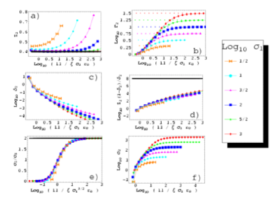
Figure 2: Several downstream parameters obtained by numerical solution of the jump conditions. The ratio $Z_{2}=n_{\rm c2}/n_{\rm h2}$ is shown in Fig a), the downstream Lorentz factor in Fig b), the downstream relative current sheet thickness in Fig c). The fraction of cold to hot plasma component after shock crossing, evaluated by Eq. (49) is shown in Fig d). Even in the low dissipation limit, it is not equal to the upstream fraction, denoted by solid thick line at $10^{8}$, see Eq. (50). The ratio of downstream to upstream magnetisation $\sigma_{2}/\sigma_{1}$ is shown in Fig e), the downstream magnetisation in Fig f). Note that for the ratio $\sigma_{2}/\sigma_{1}$, the abscissa scales like $\sigma^{-3/2}$ in order to overlap all curves independently of $\sigma_{1}$ and to match condition (42). All quantities except for fig e) are plotted versus the adimensional parameter $l_{1}/\xi\,\sigma_{1}\,r_{0}$. Different colors associated with different symbols represent different $\log_{10}\,\sigma_{1}$ as detailed in the legend. The asymptotes in the limit of no dissipation (ideal MHD shock) in fig. b) are shown in colored dotted lines.

The dissipation is complete when $\delta_{2}$ approaches unity, Fig. 2c), so that the striped structure is removed. Equivalently, it corresponds to the case where $\sigma_{2}\ll 1$. Inspecting the Fig. 2f), we expect this to happen when $\sigma_{1}\geq l_{1}/\xi\,r_{0}$; so we retrieve the condition Eq. (45) for full Poynting flux dissipation. In this case, the magnetic field is converted into particle heating. The thermalisation is complete and the flow downstream is purely hydrodynamical. The total energy flux is entirely carried by the matter energy flux, $\sigma_{2}\ll 1$. Note that the region where $\delta_{2}>1$ is meaningless. This can imply some negative magnetisation for low $\sigma_{1}$ as clearly seen in Fig. 2e). The fraction of cold to hot particle densities $Z_{2}$ is close to $2/5$, fig.2 a). Actually, for sufficiently large magnetisation $\sigma_{1}$, it does not vary much and remains close to this value, let reconnection be or not. The Lorentz factor becomes close to unity $\Gamma_{2}\approx 1$, fig.2 b).

To resume, the numerical solution of the jump conditions confirm our analytical expectations summarised in Table 1. Results have been extended to less restricted upstream flows, the magnetisation being not necessarily very high. A good estimate for $Z_{2}$ is $2/5$. It is a good approximation whenever $\sigma_{1}\geq 100$, as depicted by a solid thick line in Fig. 2a).

In Fig. 2d), we plot the fraction of cold to hot plasma component given by

$$Z_{2}\,\frac{1-\delta_{2}}{\delta_{2}}$$ (49)

It is clearly seen that this ratio is not constant and much less than the upstream fraction given by

$$Z_{1}\,\frac{1-\delta_{1}}{\delta_{1}}=10^{8}$$ (50)

and shown by a solid thick line. The reason is that some magnetic dissipation occurs even at the condition (42). The amount of the energy dissipated is not sufficient to affect the jump conditions but some particles from the cold part diffuse across the magnetic field lines and enter the sheets.

In a final step, we determine the free parameter $\xi$ with help of PIC simulations. This is discussed in the next section.

4 TERMINATION SHOCK: PIC SIMULATIONS

We designed a fully relativistic and electromagnetic 1D PIC code following the algorithms described in Birdsall & Langdon (2005). Particle trajectories are advanced in time by integrating the relativistic equation of motion due to the Lorentz force. The longitudinal electric field is found by solving Poisson equation whereas the transverse component of the electromagnetic field are computed by the remaining component of Maxwell equations introducing a left and right-going wave such as $F^{\pm}=E_{\rm y}\pm c\,B_{\rm z}$, see Birdsall & Langdon (2005). The simulation is one dimensional in space along the $x$-axis and two dimensional in velocity in the plane $(xOy)$.

The striped wind propagates along the $x$-axis and hits a wall located at the right boundary of the simulation box of length $L$. We also impose no incoming electromagnetic wave at this boundary. The particle momentum vector possesses a longitudinal component $p_{\rm x}$ and a transversal component $p_{\rm y}$. They propagate from the left to the right and hit the solid wall at $x=L$. This means that particles are reflected at this boundary, the $p_{\rm x}$ momentum is reversed whereas the $p_{\rm y}$ component remains unchanged. The magnetic field is directed along the $z$-axis and reverses polarity when crossing each current sheet. Electromagnetic waves leave the simulation box at the right boundary without any reflection. Similar simulations have already been performed by Lyubarsky (2005b).

A typical initial situation showing the magnetic field structure, the lepton distribution functions, the temperature and the drift speed is shown in Fig. 3. Close to the right wall, we impose a decreasing magnetic field strength $B_{\rm z}(x)$ which almost vanishes at $x=L$, Fig. 3a). The magnetic polarity reversal is smooth, it is not squared but evolves according to the following expression

$$B_{\rm z}(x)=B_{0}\,\tanh[\Delta\,(a+b\,\cos(\lambda\,x))]\,D(x)$$ (51)

where $B_{0}$ is the maximal intensity of the magnetic field, $a$, $b$, $\lambda$ and $\Delta$ are constants, $\Delta$ prescribing the thickness of a current sheet and $\lambda$ the number of periods in the simulation box. This particular expression is dictated by the structure of the striped wind, see for instance Eq. (1) in Pétri & Kirk (2005). $D(x)$ is a function introduced to decrease the magnetic field intensity close to the wall, at $x=L$. Moreover, because magnetic pressure is balanced by gaseous pressure, the temperature $T(x)$ in the gas also decreases close to the right wall where it almost vanishes, Fig. 3d), in accordance with the magnetic field behavior. Lower temperature implies weaker spread in particle momentum space, Fig. 3b) and c) (note that we keep track of only 50.000 particles, chosen randomly at each time step, in order to avoid too large data files). We also take the bulk Lorentz factor of the flow,  $\Gamma_{1}$, decreasing near the right wall. The average longitudinal momentum $p_{\rm x}$ also decreases in relation with the decreasing $\Gamma_{1}$. With this initial condition, we avoid the formation of too large a transient when the plasma first collides with the right wall.

The plasma moves in the positive $x$ direction with the bulk Lorentz factor $\Gamma_{1}=20$. The temperature in the plasma is obtained from the equilibrium conditions, namely pressure balance between gaseous and magnetic part. In the current sheet, the temperature is much higher than in the magnetised part, Fig. 3d). This implies a much larger spread in momentum as seen in Fig. 3b) and c). The average magnetic field $\alpha=<B>/B_{0}$ is not necessarily zero because two successive stripes generally have different width but the same magnetic field intensity $B_{0}$. In the pulsar wind, the average magnetic field only vanishes in the equatorial plane, $\theta=\pi/2$ in spherical coordinates $(r,\theta,\varphi)$. Actually, in Fig. 3a) as well as in the simulation results presented below (Fig. 4a) and Fig. 8a)), the average magnetic field is $\alpha\approx 0.12$. We choose an average value different from zero not because of numerical stability requirement but because we want to demonstrate that even in case of full dissipation the average magnetic flux downstream the shock is preserved. We also performed a set of simulations with zero average magnetic field. The results obtained are not affected and remain qualitatively the same in both cases as will be shown later. Moreover, passing from one current sheet to the next one, the drift speed for each species reverses sign, Fig. 3e). Indeed, in a current sheet, the magnetic field, oriented in the $z$ direction, is sustained by an electric current flowing in the $y$ direction. This current is generated by electrons moving in, let’s say, the positive $y$ direction at a speed $U_{s}$ whereas positrons are moving in the opposite direction at a speed $-U_{s}$. Charge neutrality is maintained but a net total current exists.

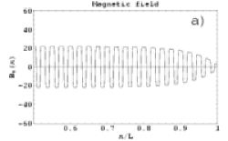
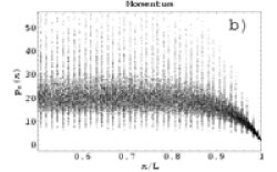
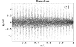
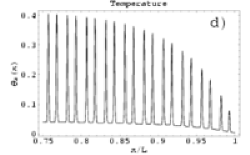
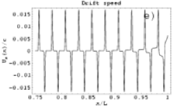
Figure 3: Initial conditions. The geometry of the striped magnetic field is shown in Fig. a). The longitudinal $p_{\rm x}$ and transversal $p_{\rm y}$ component of the momentum of one species are seen in Fig. b) and c) respectively. The temperature and the drift speed for one species (the speed of the other species is equal and opposite) are shown respectively in Fig. d) and e).

For the results presented in this section, the simulation box is divided into $2\times 10^{5}$ cells and we used $8\times 10^{5}$ particles for each species, i.e. $8\times 10^{5}$ electrons and $8\times 10^{5}$ positrons. Therefore, on average, there are only $4+4$ particles per cell. Although this number seems rather small, we checked that increasing the number of particles per cell do not improve the accuracy of our results. Thus, we performed the whole set of simulations with this resolution. To support our statement, we will show examples with $40+40$ particles per cell. The particle number density in the hot unmagnetised part, i.e. in the sheets, is five times higher than in the cold magnetised part, $n_{\rm h1}=5\,n_{\rm c1}$. The time step is chosen such that $\omega_{B}\,\Delta t=0.5$. The resulting upstream Larmor radius, deduced from this value and from $\Gamma_{1}=20$ according to Eq. (28), is equal to $r_{0}=40$ cells. Half a wavelength of the striped wind is $l_{1}=2500$ cells and the relative current sheet thickness is $\delta_{1}=0.1$. At the left boundary of the simulation box, no incoming plasma is injected. The upstream plasma is simply flowing to the right and leaves an empty space behind it with a constant magnetic field advected at the flow bulk speed $\Gamma_{1}$. In order to keep meaningful results, the simulation has to be stopped at the time $t_{\rm f}=L/2c$ before the electromagnetic wave starting at $t=0$ at the right wall reaches this vacuum region, propagating from left to right starting from $x=0$ at $t=0$.

In all runs, the simulation box starts with a inhomogeneous plasma made of electrons and positrons following a 2D relativistic Maxwellian distribution function in their proper frame given by

$$f_{s}(x,p_{\rm x},p_{\rm y})=\frac{N_{s}}{2\,\pi}\,\frac{e^{-(\gamma-1)/\Theta_{s}}}{m_{s}^{2}\,c^{2}\,\Theta_{s}\,(1+\Theta_{s})}$$ (52)

with relativistic temperature $\Theta_{s}=k_{\rm B}\,T_{s}/m_{s}\,c^{2}$ and Lorentz factor $\gamma=\sqrt{1+(p_{\rm x}^{2}+p_{\rm y}^{2})/m_{s}^{2}\,c^{2}}$. The temperature $\Theta_{s}$ is obtained from the pressure equilibrium condition Eq. (6) and shown in Fig. 3d). $N_{s}$ is the particle number density in the proper frame, $m_{s}$ the mass of a particle of each species. Because they are equal for electrons and positrons, we note $m_{s}=m$. We have to distinguish between 3 reference frames

• $R_{\mathrm{s}}$: the species frame or proper frame of reference for each species, electrons and positrons, in which the distribution function is given by the 2D relativistic Maxwellian Eq. (52) ;

• $R_{\mathrm{w}}$: the wind frame of reference in which the leptons are counter-streaming with velocity $\pm U_{s}$ ;

• $R_{0}$: the observer frame or simulation box frame or lab frame of reference in which the wind (the current sheets) is propagating in the positive $x$-direction with a Lorentz factor $\Gamma_{1}$.

To upload the initial distribution function of each species in the lab frame, we have to make two successive Lorentz transformations, the first one leading from $R_{\mathrm{s}}$ to $R_{\mathrm{w}}$ and the second one leading from $R_{\mathrm{w}}$ to $R_{0}$.

We performed many runs with different initial Lorentz factor of the wind and different magnetisation. We give a typical sample of runs demonstrating full dissipation of the magnetic field or no dissipation at all.

Because the velocity space is only two-dimensional in our simulations, see the distribution function Eq. (52), the adiabatic index for the relativistic plasma is $\gamma=3/2$ instead of the usual $4/3$. This different index will affect the parameters downstream the shock like the temperature, the Lorentz factor and the magnetisation. The general jump conditions for arbitrary adiabatic index are derived in appendix A. These formulae will help us to make quantitative comparisons between the analytical results presented before (and made for $\gamma=4/3$) and the PIC simulations.

4.1 Negligible dissipation

Here we show details of a typical example where magnetic dissipation is negligibly small. The magnetisation between the sheets is set to $\sigma=3$. It corresponds to the definition of $\sigma_{1}$ in Eq. (1). The true magnetisation Eq. (53), equal to $\sigma\approx 2.7$, differs from the one in the cold part $\sigma$ because in our PIC simulations, we need to resolve the structure of the sheet (sheet thickness larger than the Larmor radius) therefore the contribution from the cold unmagnetised part is not negligible. The true average magnetisation is actually roughly 10% lower than the one in the cold part due to the relative current sheets thickness $\delta_{1}=0.1$. The true magnetisation, averaged over one wavelength of the striped wind , is given in the rest frame of the downstream plasma by

$$\langle\sigma\rangle=\frac{\langle\mathrm{electromagnetic\;\;energy\;\;density}\rangle}{\langle\mathrm{enthalphy\;\;density}\rangle}$$ (53)

For a fluid with adiabatic index $\gamma=3/2$, the average enthalpy density (in the rest frame) is given by

$$\langle\mathrm{enthalphy\;\;density}\rangle=3/2\,\langle\mathrm{internal\;\;energy\;\;density}\rangle-1/2\,\langle\mathrm{particle\;\;number\;\;density}\rangle\,c^{2}$$ (54)

The internal energy includes the rest mass energy as well as the kinetic energy of the particles. This formula is only valid in the rest frame of the fluid. In our computations, the frame of the simulation box corresponds to the rest frame of the downstream plasma, therefore Eq. (54) applies to this plasma but not to the upstream one which moves with a Lorentz factor $\Gamma_{1}$ with respect to the simulation box. Thus, we have first to transform back to the rest frame of the upstream plasma and then apply Eq. (53) and (54). The upstream rest frame is easily found because we impose the Lorentz factor of the upstream plasma with respect to the simulation box which is also the rest frame of the downstream plasma. Therefore, the Lorentz transform in the upstream frame involves simply $\Gamma_{1}$. Note however that this is correct only well upstream and not in the shock itself. The bulk Lorentz factor differs from $\Gamma_{1}$ whenever a precursor arrives. Nevertheless, we are only interested in the average quantities when the front shock has passed through the plasma. The precise values within the shock front are not significant for our study. Note that the true local wavelength upstream as well as downstream the shock, necessary for the averaging $<>$ in Eq. (53) and (54), is determined by looking for the locations where the magnetic field vanishes. Indeed, due to compression of the plasma after shock crossing, the length of the stripes downstream are reduced by a factor $\beta_{1}/\beta_{2}(x)>1$ compared to their value upstream, according to Eq. (15). Note also that the downstream wavelength can vary slightly (a few percent) from one period to the next one, due to some perturbations. These perturbations propagate also in the upstream flow, causing some small changes in the upstream wavelength too. All these variations are taken into account when computing the averaged quantities presented in the figures.

The results of the run are summarised in Fig. 4 for a final time of simulation $t_{\rm f}=L/2\,c=5\times 10^{4}$. This corresponds to the time needed by an electromagnetic wave to propagate from the wall at the right boundary, starting at $t=0$ and arriving at the middle of the simulation box $L/2$ at the time $t_{\rm f}$. The shock front is very sharp with a very small thickness and located at approximately $x/L\approx 0.62$. It propagates in the negative $x$ direction, starting from the wall located at the right boundary as before. Looking at the structure of the magnetic field, Fig. 4a), the stripes downstream are perfectly preserved. They are still clearly recognisable in Fig. 4b) and c). They are only subject to a compression of a factor roughly equal to two. Thus the wavelength of the wind in the downstream frame has been divided by two whereas the magnetic field strength, due to magnetic flux conservation, increases by a factor two. The mean particle density in the shocked plasma, Fig. 4e), reaches a value close to two, in accordance with the magnetic field compression ratio of two. Because we average over one wavelength of the striped wind, the difference in hot and cold density is smoothed out.

The factor two can be explained as follows. The shock propagates with velocity close to c. In the shock frame, the magnetic field strength and the particle number density remain nearly the same, $B_{2}=B_{1}$ and $n_{2}=n_{1}$ (in the high $\sigma$ limit the shock is weak!). However, in the simulation frame, which is the downstream frame, they vary because of Lorentz transformations. Indeed, let’s note $n_{1/2}$ the density of the upstream plasma, proper density $n_{1}^{\prime}$, as measured in the rest frame of the downstream plasma. Let also $\Gamma_{1/2}$ be the relative Lorentz factor of the incoming flow as measured in the shocked plasma. It is easy to show that a Lorentz transformation gives

$$\Gamma_{1/2}=\Gamma_{1}\,\Gamma_{2}\,(1-\beta_{1}\,\beta_{2})$$ (55)

Thus the upstream density as measured in the downstream plasma is

$$n_{1/2}=\Gamma_{1/2}\,n_{1}^{\prime}$$ (56)

With help of the jump condition for particle number density conservation, we found

$$\frac{n_{2}^{\prime}}{n_{1/2}}=\frac{\Gamma_{1}\,\beta_{1}}{\Gamma_{1/2}\,\Gamma_{2}\,\beta_{2}}$$ (57)

In the ultra-relativistic limit, $\beta_{1}\to 1$, we get

$$\frac{n_{2}^{\prime}}{n_{1/2}}\approx\frac{1+\beta_{2}}{\beta_{2}}$$ (58)

Therefore the factor 2 when $\beta_{2}\approx 1$. Actually, because the magnetisation is not very high, $\sigma_{1}=3$, in the shock frame, the downstream plasma propagates with a Lorentz factor $\Gamma_{2}\approx\sqrt{5\,\sigma_{1}/4}$ (see appendix A), corresponding to a speed $\beta_{2}=0.86$. Inserting this value in Eq. (58), we found $n_{2}^{\prime}/n_{1/2}\approx 2.15$, very close to the average density in the shocked plasma, see Fig. 4e). Therefore, the shock front propagates in the negative $x$-direction with the speed $\beta_{2}$. Starting from $t=0$ at $x=L$, at the end of our simulation, it traveled a distance $\Delta x=\beta_{2}\,c/2*t_{\rm f}\approx 0.43\,L$. Therefore the shock front should be located at $x/L=0.57$. However, the magnetisation at the initial time close to the wall is very weak, close to unity. Therefore, the shock speed is smaller at earlier times. That is why the shock front is located at only $x/L\approx 0.62$ as can be checked by inspecting Fig. 4a) and b) and c) where a sharp transition is observed between the upstream and downstream flow.

Another way to estimate the speed of the shock is to compare the position of the shock front at the final snapshot, ($x/L\approx 0.62$) and at the penultimate snapshot ($x/L\approx 0.664$). Moreover, the time between these two snapshots is $\Delta t=L/20\,c$. Therefore, the speed of the shock front is roughly $\beta_{2}\approx 0.044\,L/(L/20)\approx 0.88$, close to the estimate made above.

The particles downstream are not thermalised. Indeed, the particle momentum which is mainly directed along the propagation axis of the wind in the upstream flow, $p_{\rm y}\ll p_{\rm x}$, is only weakly disturbed by the shock. The magnitude of $p_{\rm x}$ is not altered by the shock. Nevertheless, after crossing the shock, both longitudinal and transversal momenta are of the same order of magnitude, $p_{\rm y}\approx p_{\rm x}$. The mean particle Lorentz factor, $\gamma$, is roughly increased by a factor of two, Fig. 5. Although the transition for the transverse momentum component is very sharp, the stripes are still clearly identifiable, Fig. 4b) and c). The magnetisation downstream is increased by a factor roughly equal to two, as expected from the analysis of Sect. 3, Fig. 4d), demonstrating that the magnetic field does not dissipate.

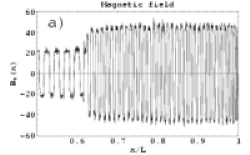
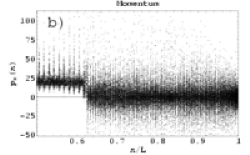
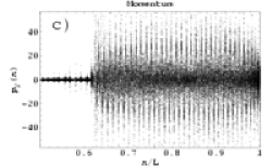
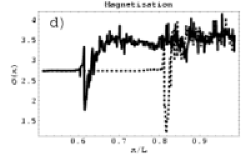
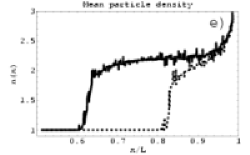
Figure 4: Example of run showing no magnetic reconnection at the termination shock. The Lorentz factor of the wind is $\Gamma=20$ and the magnetisation $\sigma=3$. The magnetic field is shown in Fig. a), the particle longitudinal and transverse momentum component in Fig. b) and c) respectively, the intermediate, $t=2.5\times 10^{4}$ (dotted line) and final, $t=5\times 10^{4}$ (solid line) downstream magnetisation in Fig. d) and the intermediate (dotted line) and final (solid line) average particle density number downstream in Fig. e). All quantities are plotted against the normalised abscissa $x/L$.

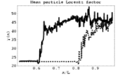
Figure 5: Mean particle Lorentz factor averaged over one period of the striped wind at an intermediate, $t=2.5\times 10^{4}$ (dotted line) and final, $t=5\times 10^{4}$ (solid line) time of simulation.

Contrary to the run presented in the next section, there is no electromagnetic precursor, the flow is not perturbed by the shock front. The situation is very similar to the ideal relativistic MHD shock. The magnetic field lines, frozen into the plasma, have to follow the motion imposed by the matter. The shocked plasma is compressed, and due to the frozen magnetic flux, the stripes are also compressed in the same ratio.

Increasing the number of particles per cell will not improve the accuracy. Indeed, we performed another run with ten times more particles per cell ($40+40$), see Fig. 6 and compare with Fig. 4. Therefore, using only $4+4$ particles per cell is justified.

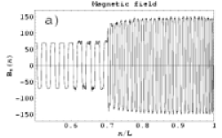
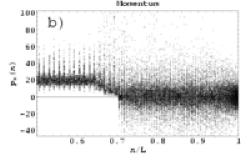
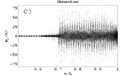
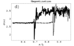
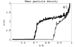
Figure 6: Same as Fig. 4 but with ten times more particles per cell, i.e. 40 positrons and 40 electrons per cell. The results are nearly the same as in Fig. 4. However, we stopped the run when made sure that everything proceeds like the run with $4+4$ pairs so that the position of the shock is different.

Finally, we show an example with zero average magnetic field $\alpha=0$ in Fig. 7 to prove that this parameter $\alpha$ does not affect much the flow downstream provided $\alpha\ll 1$.

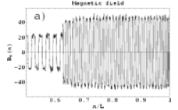
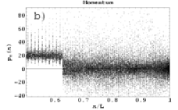
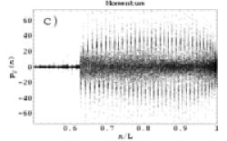
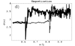
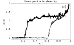
Figure 7: Same as Fig. 4 but with zero average magnetic field, $\alpha=0$. The results are nearly the same as in Fig. 4.

4.2 Full dissipation

In this paragraph, we discuss in detail a typical example of full magnetic reconnection in the striped wind. The magnetisation in the cold magnetised part, i.e. between the sheets, is set to $\sigma=45$. The true average magnetisation, $\sigma_{1}\approx 40.0$, is here again roughly 10% lower than the one in the cold part due to the relative current sheets thickness $\delta_{1}=0.1$.

The only change we made compared to the previous case is to take a higher magnetisation. This has dramatic consequences on the flow downstream as we will see now.

The simulation results are shown in Fig. 8 for the final time $t_{\rm f}=L/2\,c=5\times 10^{4}$. At this snapshot, the shock front is located at approximately $x/L\approx 0.75$ (see below how this location was determined). It propagates in the negative $x$ direction, starting from the wall located at the right boundary $x=L$. Looking at the structure of the magnetic field, Fig. 8a), it is clearly seen that the stripes, after crossing the shock are destroyed. Nevertheless, because the average magnetic field does not vanish, a small DC component remains, of the order of $\alpha=0.12$. The particles downstream are fully thermalised. Indeed, in the upstream flow corresponding to $x/L<0.78$, the particle momentum is mainly directed along the propagation axis of the wind, longitudinal momentum $p_{\rm x}$ depicted in Fig. 8b), with non negligible transverse momentum $p_{\rm y}$ only within the current sheets, Fig. 8c). The upstream longitudinal component $p_{\rm x}$ is by orders of magnitude larger than the transverse component $p_{\rm y}$, $p_{\rm y}\ll p_{\rm x}$. The particle momentum distribution function is randomised when crossing the shock discontinuity, i.e. in the region defined by $x/L>0.75$, and therefore downstream the two component of the momentum are of the same order of magnitude, $p_{\rm y}\approx p_{\rm x}$ and by orders of magnitude larger than before the shock. The enhancement in the momentum of the particle in both directions, $p_{\rm x}$ and $p_{\rm y}$, is explained by the Poynting flux dissipation. Magnetic energy is converted into particle kinetic energy. There are no more spikes in the $p_{\rm x}$ graph proving that the stripes disappeared. The magnetisation downstream is almost zero, solid curve in Fig. 8d), indicating that the alternating magnetic field has completely dissipated into particle heating as expected. In that case, the flow downstream is hydrodynamical and the compression ratio close to three. The mean particle density in the shocked plasma, solid curve in Fig. 8e), indeed reaches a value close to three.

The factor three can be explained in the following way. Assuming full dissipation of the magnetic field, the upstream flow is strongly magnetised whereas the downstream plasma is purely hydrodynamical. For an ultra-relativistic gas, the adiabatic index is $\gamma=4/3$. This is true for particles evolving in a three dimensional velocity space in which they possess three degree of freedom in translation motion. However, in our simulations, the distribution function, Eq. (52), is only two-dimensional in velocity space and the corresponding adiabatic index is thus $\gamma=3/2$. Solving the MHD jump conditions for this 2D plasma, it is easily found that the downstream plasma velocity in the rest frame of the shock is $\beta_{2}=1/2$ (2D velocity space) instead of the traditional $\beta_{2}=1/3$ (3D velocity space). Using Eq. (58), the ratio of the particle number density expressed in the downstream frame (simulation box frame) is $n_{2}^{\prime}/n_{1/2}=3$ as expected. Again, the front shock propagates in the negative $x$-direction with the speed $\beta_{2}=1/2$. Starting from $t=0$ at $x=L$, at the end of our simulation, it traveled a distance $\Delta x=c/2\,t_{\rm f}=L/4$. Therefore the shock front should be located at $x/L=0.75$. However, because of some small retardation effect to initiate the shock front, it is seen to lie at $x/L\approx 0.78$ by inspecting Fig. 8a) and b) and c).

It is also interesting to note that the incoming flow is already perturbed before entering the shock. The magnetisation gradually decreases and becomes already very small in the region just before the shock discontinuity. The stripes start to be significantly disturbed already at $x/L\approx 0.6$. This phenomenon is probably due to an electromagnetic precursor, i.e. and electromagnetic wave generated at the shock front and propagating downwards into the upstream plasma (Hoshino et al., 1992; Gallant et al., 1992). Moreover, from the momentum component $p_{\rm x}$, we conclude that the flow is heated already well upstream of the shock. If the strong electromagnetic precursor would be generated immediately at the initial time $t=0$, we would expected it to influence half of the simulation box from $x/L=0.5$ to $x/L=1$ at the final time $t_{\rm f}$. However, the amplitude of the precursor is initially small because due to the chosen initial distribution of the flow parameters (Fig.3), the energy of the plasma entering the shock is initially small. The strong shock is formed after some time (about 0.05L/c) when the highly relativistic plasma enters the shock. Thus a strong enough precursor is generated not from the beginning of the simulations and therefore the flow is significantly perturbed at $x/L\gtrsim 0.55$.

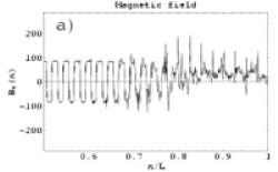
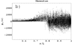
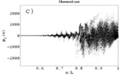
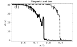
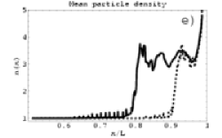
Figure 8: Example of run showing the magnetic reconnection at the termination shock. The Lorentz factor of the wind is $\Gamma=20$ and the magnetisation $\sigma=45$. The same quantities as in Fig. 4 are plotted.

The effect of a precursor was not included in our analytic analysis. It is performed with the assumption that the dissipation is weak; in this case, there is no significant precursor. In any case, our analysis is valid provided the downstream flow is settled into a striped wind. Then we apply the conservation laws to flows well upstream and well downstream of the shock and processes within the “black box” containing the shock and possible precursors do not affect the results.

In case of high upstream magnetisation, the flow in the wind is dominated by the dynamics of the magnetic field, i.e. gaseous pressure negligible compared to magnetic pressure. Therefore the shocked plasma has to reorganise in such a way to keep the striped structure. If this plasma is unable to maintain the current required by the magnetic field, the latter will dissipate.

Finally, here again, we show an example with zero average magnetic field $\alpha=0$ in Fig. 9. One sees that the Poynting flux dissipates completely in this case also. However there is no sharp shock transition in this case. When the average magnetic field is nonzero, the shock is mediated by the Larmor rotation of particles and the width of the shock transition is roughly equal to the Larmor radius in the average field, $r_{0}/\alpha$. In our simulations this is $40/\alpha$ cells so that even at $\alpha=0.1$ the shock transition is narrow. When $\alpha=0$, the particle free path is determined only by scattering on magnetic fluctuations therefore the shock transition could be rather wide.

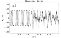
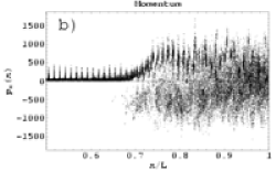
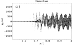
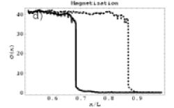
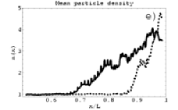
Figure 9: Same as Fig. 8 but with zero average magnetic field, $\alpha=0$.

4.3 Empirical law

In the last two paragraphs, we gave two examples of runs, the former demonstrating that the striped wind can be preserved when some conditions are fulfilled and the latter showing a case of full magnetic reconnection. We performed many simulations with different parameters, changing the magnetisation, the Lorentz factor, the Larmor radius in order to segregate between the two regimes.

The results of the full set of simulations can be summarised in plots showing the ratio of the true downstream to the true upstream magnetisation $\sigma_{2}/\sigma_{1}$ as well as $\sigma_{2}$, Fig. 10. To sum up, we obtain the curves represented in Fig. 10, where these quantities are plotted against the parameter $\eta=l/r_{0}\,\sigma^{3/2}$ and $\eta\,\sqrt{\sigma}$ for fig. a) and b) respectively and for different initial magnetisations, as was done in the semi-analytical results presented in Fig. 2 e) and f).

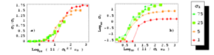
Figure 10: Empirical law for magnetic reconnection in the striped wind obtained by 1D PIC simulations. The ratio of the downstream to the upstream true magnetisation $\sigma_{2}/\sigma_{1}$ is plotted against $l/r_{0}\,\sigma^{3/2}$ in fig a) and the downstream magnetisation against $l/r_{0}\,\sigma$ in fig b) for different values of the theoretical upstream magnetisation $\sigma$ from mildly $\sigma=1$ to highly magnetised flow $\sigma=75$.

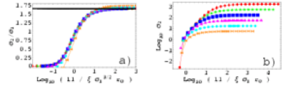
Figure 11: Same figures as Fig.2e) and f) respectively fig. a) and b) here, but for an adiabatic index $\gamma=3/2$ instead of $\gamma=4/3$.

For the largest values of $\eta$, no reconnection is observed as we would expect from the analytical study discussed in Sect. 3. In the no dissipation limit, $\eta\gg 1$, the ratio $\sigma_{2}/\sigma_{1}$ reaches values close to 1.7, in accordance with the expected $5/3$-ratio for the ideal MHD shock with $\gamma=3/2$ (see appendix A). As this limit is achieved at the same $\eta$ for any $\sigma$, we retrieve the condition Eq. (42). According to Fig 10 b) all the presented curves, with the exception of the one corresponding to $\sigma=1$, go to zero at the same condition

$$\frac{l}{r_{0}\,\sigma}\leq 3.$$ (59)

This confirms the analytical criterion 45 found at the condition $\sigma\gg 1$.

To allow detailed comparisons of the PIC simulations with the theoretical model presented in sections 2 and 3, we plotted in Fig 11 the quantities $\sigma_{2}/\sigma_{1}$ and  $\sigma_{2}$ calculated from the theoretical model with the adiabatic index  $\gamma=3/2$ (the same quantities were plotted in Figs.2e) and f) for $\gamma=4/3$). Theoretical jump conditions for arbitrary $\gamma$ are presented in Appendix B. Comparing Fig. 11 a) and Fig. 10 a) on one hand, and Fig. 11 b) and Fig. 10 b) on the other hand, the parameter $\xi$ (the ratio of the sheet width and the particle Larmor radius), introduced at the end of Sect. 2, can be easily estimated. Indeed, looking at fig.10a), we find that no dissipation occurs whenever $l/r_{0}\,\sigma^{3/2}\approx 100$ whereas fig.11a) gives $l/r_{0}\,\xi\,\sigma^{3/2}\approx 10$ so that $\xi\approx 10$. On the other hand, fig.10b) shows full dissipation at $l/r_{0}\,\sigma\approx 3$. Comparing with fig. 11b) which gives $l/r_{0}\,\xi\,\sigma\approx 0.5$, we get $\xi\approx 6$. This means that $\xi\approx 6-10$.

Finally substituting Eqs.(1) and (27) into Eq.(59), the parameter region for full dissipation is found as

$$\mu_{0}\,c\,|q|\,\frac{l\,n_{\rm c1}}{B_{1}}\leq 3$$ (60)

Note also that the condition for full dissipation Eq. (60) is independent of the upstream Lorentz factor $\Gamma_{1}$.

5 Application to pulsar winds

We apply Eq. (60) to pulsar winds. The idea is to find the limiting radius beyond which the alternating field dissipates at the termination shock. Because all quantities refer to the upstream plasma, we drop the subscript $1$.

Beyond the light cylinder, we assume that the outflow is radial and propagating in the radial direction. The magnetic field is predominantly toroidal and decreases with radius as

$$B=B_{\rm L}\,\frac{R_{\rm L}}{R}$$ (61)

where $R_{\rm L}=c/\Omega$ is the radius of the light cylinder, $\Omega$ the angular velocity of the neutron star and $B_{\rm L}$ the magnetic field strength at the light cylinder. The particle number density falls off as

$$n=n_{\rm L}\,\left(\frac{R_{\rm L}}{R}\right)^{2}$$ (62)

where the density at the light cylinder $n_{\rm L}$ is conventionally expressed via the so called multiplicity factor $\kappa$ such that

$$n_{\rm L}=2\,\varepsilon_{0}\,\kappa\,\frac{\Omega\,B_{\rm L}}{|q|}$$ (63)

Half of a wavelength in the striped wind is given by $l=\pi\,R_{\rm L}$. Substituting these relations into Eq.(60), one finds that full magnetic dissipation occurs at the termination shock whenever the shock arises at the distance larger than

$$\frac{R}{R_{\rm L}}\geq\frac{2\,\pi}{3}\,\kappa.$$ (64)

We suppose that the termination shock is stationary in the observer (pulsar) frame.

The value of the multiplicity, $\kappa$, is rather uncertain. The available theoretical models (Hibschman & Arons, 2001a, b), give $\kappa$ from a few to thousands. The observed synchrotron emission from the Crab nebula places wide limits on $\kappa$, from $\kappa\sim 10^{4}$, at the assumption that only high energy electrons (those emitting the optical and harder radiation) are injected now into the nebula, to $\kappa\sim 10^{6}$ if the radio emitting electrons are also injected now but not only in the early stage of the pulsar history. In any case the condition Eq. (64) is easily satisfied for plerions because the termination shock is located at radii $10^{14}-10^{16}\,{\rm m}\sim 10^{8}-10^{10}\,R_{\rm L}$ from the pulsar. For instance, in the Crab nebula, the termination shock is located at $R_{\rm shock}/R_{\rm L}=3\times 10^{9}\gg\kappa$. Thus for these pulsar wind nebulae, the magnetic energy is easily dissipated at the termination shock so that the pulsar wind could remain highly magnetised even in the upstream region close to the shock front. All the available observation limits on $\sigma$ are obtained from the analysis of the plasma flow and radiation beyond the termination shock, the necessary upstream $\sigma$ being calculated from the ideal MHD jump conditions, see for instance the recent papers by Torii et al. (2000); Safi-Harb et al. (2001); Petre et al. (2002). Our results show that even if the pulsar wind remains Poynting dominated until the termination shock, magnetic dissipation at the shock front would suffice to efficiently convert the electromagnetic energy to the plasma energy. This point of view is an alternative to the $\sigma$-problem.

In binary pulsars, interaction of the pulsar wind with the companion star results in formation of an intra-binary shock very close to the neutron star, only thousands of light cylinder radii. Arons & Tavani (1993); Tavani & Arons (1997); Cheng et al. (2006) claim that the X-ray emission observed from the binary pulsars PSR 1957+20 and PSR 1259-63 is explained if the magnetisation downstream of the shock is small so that the Poynting flux is already converted into the plasma energy. Then we could estimate from Eq.(64) the upper limit of the pair production factor $\kappa$ for these pulsars.

Indeed, first consider the pulsar PSR 1957+20. It has a rotation period of $P=1.607$ ms, corresponding to a light cylinder radius of $R_{\rm L}=76.7$ km. The intra-binary shock arises at a distance less than the orbital separation to the companion star, so that we get $R_{\rm shock}\lesssim 1.7\times 10^{6}$ km. According to Eq. (64), in order to expect a significant dissipation of the magnetic field at the shock, the multiplicity factor should then satisfy $\kappa\leq(1/\pi)\,R_{\rm shock}/R_{\rm L}\approx\times 10^{4}$.

Next consider the pulsar PSR 1259-63. It possesses a period of $P=47.7$ ms, corresponding to a light cylinder radius $R_{\rm L}=2279$ km. Because here again the shock should arise at a distance smaller than the orbital separation, we found $R_{\rm shock}\lesssim 3.9\times 10^{8}$ km. Magnetic reconnection implies $\kappa\lesssim 8\times 10^{4}$.

Another interesting case is the famous double pulsar PSR J0737-3039. According to McLaughlin et al. (2004), the radio emission from the pulsar B is modulated with the period of pulsar A. This strongly supports the idea that the magnetosphere of pulsar B is disturbed by the striped wind emanating from pulsar A. The condition that the striped structure has not been erased at the distance separating both pulsars, imposes a lower limit on the multiplicity factor $\kappa$ in this case. Let us estimate this limit. The period of pulsar A is $P_{A}=22.699$ ms corresponding to a light cylinder radius of $R_{\rm L}=1083$ km. The separation between the two pulsars is approximately $700,000$ km (Lyne & Kramer, 2005). Then the lower limit for the ratio in Eq. (64) is $R/R_{\rm L}\approx 646$. We conclude that the lower limit for the pair production multiplicity in pulsar A is $\kappa\gtrsim 310$.

6 CONCLUSION

In this paper, we studied the magnetic reconnection process at the termination shock in the pulsar striped wind. Using the jump conditions for the averaged quantities (over a wavelength) in the striped wind, we derived a simple analytical criterion for magnetic dissipation, see Table 1. However, we had to introduce a free parameter $\xi$, Eq. (38), entering the dissipation condition. It relates the downstream thickness $\Delta_{2}$ of a current sheet to the downstream Larmor radius $r_{0}$ by the following expression $\Delta_{2}=\xi\,r_{0}$. $\xi$ is the only free parameter in our model. In order to estimate this parameter, we performed 1D relativistic PIC simulations and found that $\xi\approx 10$.

Knowing the important flow parameters in the incoming plasma which are half the wavelength $l$, the magnetisation $\sigma$ and the Larmor radius $r_{0}$, we are able to predict the percentage of magnetic reconnection in the striped wind when crossing the termination shock, according to the following law

• for $l/r_{0}\,\sigma\leq 3$, full dissipation occurs, the flow downstream is purely hydrodynamical with Lorentz factor close to unity $\Gamma_{2}\approx 1$, particle are thermalised and heated to relativistic temperature. The magnetic field has completely disappeared, except for the DC component (i.e. average magnetic field) ;

• for $\sigma\leq(l/12\,r_{0})^{2/3}$, no magnetic reconnection exists. The striped wind structure is preserved downstream, it is just compressed. The downstream Lorentz factor is the same as for ideal MHD, $\Gamma_{2}=\sqrt{\sigma}$ ;

• $3\leq l/r_{0}\,\sigma\leq 12\,\sqrt{\sigma}$, the magnetic field is partially dissipated. The stripes are weakened and the flow is decelerated to a downstream Lorentz factor $\Gamma_{2}=l/(12\,r_{0}\,\sigma)$.

We applied the condition for full magnetic dissipation, Eq. (64), to pulsar wind nebula and binary pulsars. Because in plerions the termination shock is located at radii $10^{14}-10^{16}\,{\rm m}\sim 10^{8}-10^{10}\,R_{\rm L}$ from the pulsar, magnetic reconnection is easily achieved. This conclusion could resolve a long-standing difficulty with transformation of the electro-magnetic energy of the pulsar wind into the plasma energy in the nebula (the so called $\sigma$-problem). First of all, both observations of the X-ray tori (Weisskopf et al., 2000) and theoretical models (Bogovalov, 1999) suggest that most of the energy in the pulsar wind is transferred in the equatorial belt where the magnetic field is predominantly alternating. We see now that even though dissipation of the alternating fields in the wind is hampered by relativistic slowing-down of time (Lyubarsky & Kirk, 2001; Kirk & Skjæraasen, 2003), the electro-magnetic energy is readily released at the terminating shock.

Our model could be applied also to pulsars in binary systems, where interaction of the pulsar wind with the companion star results in a formation of a shock relatively close to the pulsar. In this case, the presence or absence of magnetic dissipation imposes a strong constraint on the pair multiplicity factor $\kappa$. For pulsars PSR 1259-63 and PSR 1957+20, where full dissipation is expected, the upper limit is roughly $\kappa\lesssim{\rm few}\times 10^{4}$. For the binary pulsar PSR 0737-3039, we do not expect full reconnection and therefore the lower limit is found to be $\kappa\gtrsim 310$.

The generation of electromagnetic waves at the shock front and their propagation in the upstream plasma will affect the flow already before entering the discontinuity. This aspect of the reconnection in the termination shock is left for future work.

Appendix A Jump conditions for arbitrary adiabatic index $\gamma$

A.1 Ideal MHD

In this appendix, we give the general expressions for the ideal MHD jump conditions for arbitrary adiabatic index $\gamma$, (Gallant et al., 1992; Hoshino et al., 1992). Let’s assume that the equation of state for the ultrarelativistic plasma is given by

$$e=\frac{p}{\gamma-1}$$ (65)

for an arbitrary index $\gamma$. The enthalpy is therefore given by

$$w=\frac{\gamma\,p}{\gamma-1}$$ (66)

Following the procedure of Kennel & Coroniti (1984a), the solutions to the MHD jump conditions for the 4-velocity gives

$$u_{2}^{2} = \frac{(4-\gamma)\,\gamma\,\sigma_{1}^{2}+4\,(1+(\gamma-1)^{2})\,\sigma_{1}+4\,(\gamma-1)^{2}}{8\,\gamma(2-\gamma)\,(\sigma_{1}+1)}$$

$$\pm\frac{\sqrt{16\,\gamma\,(\gamma-2)^{3}\,\sigma_{1}^{2}\,(\sigma_{1}+1)+[(\gamma-2)^{2}\,\sigma_{1}^{2}-4\,(\sigma_{1}+1)\,(\sigma_{1}+(\gamma-1)^{2})]^{2}}}{8\,\gamma(2-\gamma)\,(\sigma_{1}+1)}$$

Starting from the 4-velocity, we can compute the Lorentz factor, the downstream temperature and the magnetisation by

$$\Gamma_{2} = \sqrt{1+u_{2}^{2}}$$ (68)

$$\frac{k_{B}\,T_{2}}{\Gamma_{1}\,m\,c^{2}} = \frac{\gamma-1}{\gamma}\,\frac{1}{\Gamma_{2}}\,\left[1+\sigma_{1}\,\left(1-\frac{1}{\beta_{2}}\right)\right]$$ (69)

$$\sigma_{2} = \frac{\gamma-1}{\gamma}\,\frac{n_{2}}{n_{1}}\,\frac{\Gamma_{1}}{\Gamma_{2}}\,\frac{m\,c^{2}}{k_{B}\,T_{2}}\,\sigma_{1}$$ (70)

$$\frac{n_{2}}{n_{1}} = \frac{1}{\beta_{2}}$$ (71)

For $\gamma=4/3$ we retrieve the usual result

$$u_{2}^{2}=\frac{8\,\sigma_{1}^{2}+10\,\sigma_{1}+1\pm\sqrt{64\,\sigma_{1}^{4}+128\,\sigma_{1}^{3}+84\,\sigma_{1}^{2}+20\,\sigma_{1}+1}}{16\,(\sigma_{1}+1)}$$ (72)

For arbitrary $\gamma$, the expansion in $1/\sigma_{1}$ to the second order leads to

$$u_{2}^{2}=\frac{\gamma-4}{4\,(\gamma-2)}\,\sigma_{1}-\frac{\gamma^{2}-8\,\gamma+8}{4\,\left(\gamma^{2}-6\,\gamma+8\,\right)}$$ (73)

The corresponding Lorentz factor is to the same order

$$\Gamma_{2}=\frac{1}{2}\,\sqrt{\frac{(\sigma_{1}+3)\,\gamma^{2}-8\,(\sigma_{1}+2)\,\gamma+8\,(2\sigma_{1}+3)}{\gamma^{2}-6\,\gamma+8}}$$ (74)

This leads to a downstream temperature

$$\frac{k_{B}\,T_{2}}{\Gamma_{1}\,m\,c^{2}}=\frac{\gamma-1}{4-\gamma}\,\sqrt{\frac{\gamma-2}{\gamma-4}}\,\frac{1}{\sqrt{\sigma_{1}}}\,\left(2-\frac{\gamma^{3}\,\left(3\,\gamma^{2}-8\,\gamma+8\right)}{(\gamma-4)^{2}\,\gamma^{3}}\,\frac{1}{\sigma_{1}}\right)$$ (75)

a density jump

$$\frac{n_{2}}{n_{1}}=1+2\,\frac{\gamma-2}{\gamma-4}\,\frac{1}{\sigma_{1}}$$ (76)

and a magnetisation

$$\sigma_{2}=\left(\frac{4-\gamma}{\gamma}\,-2\,\frac{(\gamma-2)^{2}}{\gamma\,(\gamma-4)\,\sigma_{1}}\right)\,\sigma_{1}$$ (77)

In Table 2, we give the numerical values for the different coefficients for $\gamma=4/3$ and $\gamma=3/2$.

Quantity	$\gamma=4/3$	$\gamma=3/2$
$\Gamma_{2}$	$\sqrt{\sigma_{1}+\frac{9}{8}}$	$\sqrt{\frac{5}{4}\,\sigma_{1}+\frac{27}{20}}$
$k_{B}\,T_{2}/m\,c^{2}$	$\frac{\Gamma_{1}}{16\,\sqrt{\sigma_{1}}}\,\left(2-\frac{3}{8\,\sigma_{1}}\right)$	$\frac{\Gamma_{1}}{5\,\sqrt{5\,\sigma_{1}}}\,\left(2-\frac{11}{25\,\sigma_{1}}\right)$
$n_{2}/n_{1}$	$1+\frac{1}{2\,\sigma_{1}}$	$1+\frac{2}{5\,\sigma_{1}}$
$\sigma_{2}/\sigma_{1}$	$2+\frac{1}{4\,\sigma_{1}}$	$\frac{5}{3}+\frac{2}{15\,\sigma_{1}}$

Table 2: Downstream parameters for the two adiabatic indexes $\gamma=4/3,3/2$, expanded to first order in the upstream magnetisation $1/\sigma_{1}$.

A.2 Striped wind

We now give the general formulae for the jump conditions in the striped wind for arbitrary adiabatic index $\gamma$. Following the same procedure as in Sect 2 using the general expression described in the previous section, the average conservation of particle and energy-momentum read,

$$\beta_{1}\,\left[(1-\delta_{1})\,n_{\rm c1}+\delta_{1}\,n_{\rm h1}\right] = \beta_{2}\,\left[(1-\delta_{2})\,n_{\rm c2}+\delta_{2}\,n_{\rm h2}\right]$$ (78)

$$\beta_{1}\,n_{\rm c1}\,\left[1-\delta_{1}+\left(\frac{2-\gamma}{2\,(\gamma-1)}\,\delta_{1}+1\right)\,\sigma_{1}\right] = \beta_{2}\,n_{\rm c2}\,\left[\frac{\gamma}{4-\gamma}+\left(1+\frac{2-\gamma}{2\,(\gamma-1)}\,\delta_{2}\right)\,\frac{n_{\rm c2}}{n_{\rm c1}}\,\sigma_{1}\right]$$ (79)

$$n_{\rm c1}\,\left[\Gamma_{1}\,\beta_{1}^{2}\,\left(1-\delta_{1}+\left(\frac{2-\gamma}{2\,(\gamma-1)}\,\delta_{1}+1\right)\,\sigma_{1}\right)+\frac{\sigma_{1}}{2\,\Gamma_{1}}\right] = \frac{\Gamma_{1}}{\Gamma_{2}}\,n_{\rm c2}\,\left[\Gamma_{2}\,\beta_{2}^{2}\,\left(\frac{\gamma}{4-\gamma}+\left(1+\frac{2-\gamma}{2\,(\gamma-1)}\,\delta_{2}\right)\,\frac{n_{\rm c2}}{n_{\rm c1}}\,\sigma_{1}\right)+\right.$$ (80)

$$\left.\frac{\gamma-1}{4-\gamma}\,\frac{1}{\Gamma_{2}}+\frac{n_{\rm c2}\,\sigma_{1}}{2\,n_{\rm c1}\,\Gamma_{2}}\right]$$

The prescription for the current sheet thickness downstream is

$$\delta_{2}=\xi\,\left[\frac{\gamma-1}{4-\gamma}+\frac{n_{\rm c2}\,\sigma_{1}}{2\,n_{\rm c1}}\right]\,\frac{\beta_{1}\,n_{\rm c1}}{\Gamma_{2}\,\beta_{2}\,n_{\rm h2}}\,\frac{r_{0}}{l_{1}}$$ (81)