A purely reflective
large wide-field telescope

Abstract — Two versions of a fast, purely reflective Paul-Baker type telescope are discussed, each with an 8.4-m aperture, $3^{\circ}$ diameter flat field and $f$/1.25 focal ratio.

The first version is based on a common, even asphere type of surface with zero conic constant. The primary and tertiary mirrors are 6th order aspheres, while the secondary mirror is an 8th order asphere (referred to here for brevity, as the 6/8/6 configuration). The $D_{80}$ diameter of a star image varies from $0^{\prime\prime}.18$ on the optical axis up to $0^{\prime\prime}.27$ at the edge of the field ($9.3-13.5\,\mu$m).

The second version of the telescope is based on a polysag surface type which uses a polynomial expansion in the sag $z$,

$$r^{2}=2R_{0}z-(1+b)z^{2}+a_{3}z^{3}+a_{4}z^{4}+\ldots+a_{N}z^{N},$$

instead of the common form of an aspheric surface. This approach results in somewhat better images, with $D_{80}$ ranging from $0^{\prime\prime}.16$ to $0^{\prime\prime}.23$, using a lower-order 3/4/3 combination of powers for the mirror surfaces. An additional example with 3.5-m aperture, $3^{\circ}.5$ diameter flat field, and $f$/1.25 focal ratio featuring near-diffraction-limited image quality is also presented.

Key words: General optics, telescopes

Introduction

Widening the field of view of large telescopes has been an active research topic during last few years. The special attention was given to further development of the Mersenne [1636] system in a direction specified by Schmidt [1930], resulting in a three-mirror telescope system. The important milestones on this path were the works of Paul [1935], Baker [1969], Willstrop [1984], and Angel et. al. [2000].

Curved focal surfaces, which are frequently encountered in wide-field designs, remain undesirable for use with modern detectors (Ackermann, McGraw, and Zimmer 2006). As is well known, there are no practical flat-field configurations for a Cassegrain system. The use of a lens corrector in the exit pupil of a Gregory system enables to reach the $\sim 3^{\circ}$ field, however it remains slightly curved (Terebizh 2006). An excellent aberration-free solution by Korsch [1972, 1977] provides the flat-field three-mirror designs in a frame of theory of 3rd-order aberrations, i.e., for the relatively slow systems. It was shown by Baker [1969] that a flat field could be attained with a fast three-mirror telescope proposed by Paul [1935] (see the general discussion in the book by Schroeder [2000], §6.4).

Our goal was to find a purely reflecting fast three-mirror system with a flat field not less than $3^{\circ}$ in diameter using only low-order aspheres. For convenience, we consider examples of such a telescope with the physical parameters close to those for the Large Synoptic Survey Telescope (LSST, see Angel et. al. 2000, Seppala 2002). Two versions of such an 8.4-m, $f$/1.25 telescope are discussed. The first telescope is based on the common, even asphere type surfaces with zero conic constant; the second version is based on a polysag type surface, which uses a polynomial expansion in the sag $z$, instead of the common form of an aspheric surface.

8.4-m telescope based on even aspheres

The design is shown in Fig. 1, with performance as described in Table 1, and the complete optical prescription given in Table A1 of the Appendix. The prescription follows the notation used by the ZEMAX optical design program. Fig. 2 presents the corresponding spot diagrams.

As one can see from Table A1, all three mirrors are even aspheres with zero conic constants, i.e., the slightly deformed spheres. Unlike the LSST, where the mirrors are primarily non-spherical conic sections with the addition of small polynomial corrections up to the 10th order, the telescope described here uses the polynomial terms comparable with the ”seed” spheres. As a consequence, the effective radius of curvature at the vertex of each surface is noticeably different from that of the sphere as seen in Table A1. In this sense, our design is closer to the Willstrop [1984] design with only polynomial representation of the surfaces profiles.

The key point is that the optimal choice both the conic constants and polynomial coefficients leads to another form of the same basic design. Indeed, we can achieve nearly the same image quality as shown in Fig. 2 for a design with non-zero conic constants (of the order of 1) and a new set of the polynomial coefficients. A whole set of parameters simply adjust the theoretically best surface profiles given flat image. The existence of the objectively best profiles for surfaces in a three-mirror telescope with a flat focal surface appears to be natural in the context of the Schwarzschild [1905] approach to aplanatic systems and generalization of that approach to any two-mirror aplanats (Terebizh 2005). We will address this topic later in more detail.

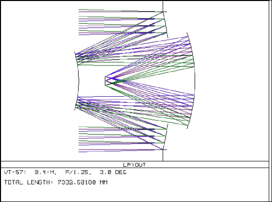
Figure 1: *

First version of a 8.4-m telescope.

Table 1. First version of the 8.4-m telescope
Parameter	Value
Entrance pupil diameter	8400 mm
Effective diameter
center of field – edge	6560 – 6470 mm
Effective focal length	10500 mm
Effective $f$-number	1.25
Scale in the focal plane	50.905 $\mu$m/arcsec
Angular field of view	$3^{\circ}.0$
Linear field of view	550.4 mm
Image RMS-diameter
center of field – edge	$0^{\prime\prime}.13-0^{\prime\prime}.19$, 6.7 – 9.8 $\mu$m
Image $D_{80}$ diameter
center of field – edge	$0^{\prime\prime}.18-0^{\prime\prime}.27$, 9.3 – 13.5 $\mu$m
Maximum distortion	0.087%
Fraction of unvignetted rays
center of field – edge	0.610 – 0.593
Orders of the aspheric mirrors	6/8/6
Length of the optical system	7333 mm

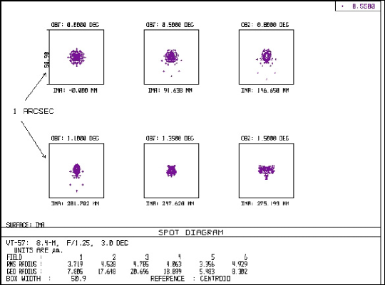
Figure 2: *

Spot diagrams of the telescope shown in Fig. 1
for the field angles $0,\,0^{\circ}.5,\,0^{\circ}.8,\,1^{\circ}.1,\,1^{\circ}.35$, and $1^{\circ}.5$.
Wavelength is $0.55\,\mu$m, the box width is $1^{\prime\prime}$ ($50.9\,\mu$m).

Table 2. Properties of the nearest spheres
	Mirror	$R_{n}$, mm	$\phi_{n}$	$\delta_{n}$, mm
Present	Primary	– 18563.048	1.105	– 1.728
design	Secondary	– 6046.431	0.854	0.0698
	Tertiary	– 9097.721	0.771	0.549
	Primary	– 17998.234	1.071	– 1.670
LSST	Secondary	– 6167.953	0.916	– 0.0696
	Tertiary	– 8411.999	0.774	– 0.214

Taking into account the above discussion concerning surface profiles, it is interesting to find their deviation from the nearest sphere. It is sufficient for our purposes to choose the simple definition of the nearest sphere, namely, the sphere that includes the surface’s vertex and outward rim. Table 2 gives the radiuses of the nearest spheres $R_{n}$, the corresponding $f$-numbers $\phi_{n}\equiv|R_{n}|/(2D_{n})$, and the maximum by modulus deviation of each surface from the nearest sphere $\delta_{n}\equiv z_{s}-z_{n}$ for the design presented here and the LSST. In general, both sets of parameters are comparable in value.

The polysag type optical surfaces

An optical surface which is symmetric about the $z$-axis is usually described by a conic section equation

$$r^{2}=2R_{0}z-(1+b)z^{2},$$

where $r=\sqrt{x^{2}+y^{2}}$ is the radial coordinate, $R_{0}$ is the paraxial radius of curvature, and the conic constant $b$ is equal to the negative of the squared eccentricity: $b=-\varepsilon^{2}$. In optical ray tracing, it is suitable to solve equation (1) with respect to the sag $z$, so the standard surface form is defined by equation

$$z=\frac{r^{2}/R_{0}}{1+\sqrt{1-(1+b)(r/R_{0})^{2}}}\,.$$

In designing fast, wide-field optical systems, the conic sections are often insufficient tools, so a polynomial in the radial coordinate is added to the sag representation (2). For example, an even asphere surface is defined as follows:

$$z=\frac{r^{2}/R_{0}}{1+\sqrt{1-(1+b)(r/R_{0})^{2}}}+\alpha_{1}r^{2}+\alpha_{2}r^{4}+\ldots+\alpha_{N}r^{2N}.$$

These surfaces are quite useful in practice, but some limitations become apparent when we enlarge the system’s aperture, speed and the field of view.

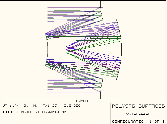
Figure 3: *

Second version of a 8.4-m telescope.

The point is that a power series slowly converges to a desired function (see, e.g., Lanczos [1988], Ch. 7; Press et. al. [1992], §5.1). In optics, we seek as proximate as possible representation of the optimal surface profile, so we are really interested in the most quickly converging series. Meanwhile, the convergence of a power representation (3) is especially slow for fast systems of large aperture, because (3) deals with powers of the ratio $r/R_{0}$, which is not particularly small near the edge of the aperture.

For these reasons, another polynomial approximation can be used to reach the better convergence. The known for a long time expansion

$$r^{2}=2R_{0}z-(1+b)z^{2}+a_{3}z^{3}+a_{4}z^{4}+\ldots+a_{N}z^{N}$$

can be considered as a natural generalization of equation (1) for the conic sections (see, e.g., Rusinov [1973]). Here $a_{3},a_{4},\ldots,a_{N}$ are coefficients which along with $R_{0}$ and $b$ define a polynomial representation in the sag $z$, but not in the radial coordinate $r$. Even for very fast surfaces, we have usually ${z\ll r}$, so the polynomial expansion in the sag (polysag) is expected to converge more quickly than (3). Besides, the direct extension of equation (1) in powers of the sag appears sometimes to be a more logical approach than adding a series in powers of $r$ to the solution of equation (1) with respect to the sag.

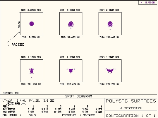
Figure 4: *

Spot diagrams of the telescope shown in Fig. 3
for the field angles $0,\,0^{\circ}.5,\,0^{\circ}.8,\,1^{\circ}.1,\,1^{\circ}.35$, and $1^{\circ}.5$.
Wavelength is $0.55\,\mu$m, the box width is $1^{\prime\prime}.0$ ($50.9\,\mu$m).

The decomposition (4) was previously tried at low orders ${N=3}$ or $4$. Modern computers enable to use the polynomial expansions of any order. The only problem is that advanced optical programs, e.g., ZEMAX, are based on the sag $z$ as a function of the radial coordinate $r$, while (4) gives the inverse relation. This problem, however, can easily be solved resulting the additional surface type, the polysag.

Examples presented below show that polysag surfaces of relatively low order allow one to design large and fast telescopes with high image quality. However, this type of surface is not universal, as sometimes it is better to treat a surface, with the aid of equation (3). An example is the corrector plate for a Schmidt camera; perhaps, the reason is that the spherical aberration of a sphere is determined just by power terms in the radial coordinate and not in the sag. Clearly, further work with the polysag type surface before limitations of its general application can be well understood.

8.4-m telescope based on polysag surfaces

Our polysag-based 8.4-m design has the same physical parameters as the first example with the traditional even asphere surfaces. The optical layout of the telescope is depicted in Fig. 3, with the corresponding spot diagrams shown in Fig. 4, and its performance and parameters given in Tables 3 and A2.

Table 3. Performance of the polysag-based telescopes
Parameter	8.4-m	3.5-m
Entrance pupil diameter	8400 mm	3500 mm
Effective diameter
center of field – edge	6561 – 6452 mm	2711 – 2711 mm
Effective focal length	10500 mm	4375 mm
Effective $f$-number	1.25	1.25
Scale in the focal plane	50.905 $\mu$m/arcsec	21.211 $\mu$m/arcsec
Angular field of view	$3^{\circ}.0$	$3^{\circ}.5$
Linear field of view	550 mm	268 mm
Image RMS-diameter
center of field	$0^{\prime\prime}.12$ (3.1 $\mu$m)	$0^{\prime\prime}.21$ (4.4 $\mu$m)
edge	$0^{\prime\prime}.18$ (9.0 $\mu$m)	$0^{\prime\prime}.30$ (6.3 $\mu$m)
Image $D_{80}$ diameter
center of field	$0^{\prime\prime}.16$ (8.3 $\mu$m)	$0^{\prime\prime}.29$ (6.1 $\mu$m)
edge	$0^{\prime\prime}.23$ (11.6 $\mu$m)	$0^{\prime\prime}.41$ (8.7 $\mu$m)
Maximum distortion	0.09%	0.12%
Fraction of unvignetted rays
center of field – edge	0.61 – 0.59	0.60 – 0.60
Orders of the aspheric mirrors	3/4/3	3/4/3
Length of the optical system	7533 mm	3485 mm

The use of the polysag-type mirrors enables the design to achieve even the better image quality on a flat field with a 3/4/3 configuration of mirrors. The image quality approximately matches atmosphere seeing with spot sizes closely matched to the size of commonly used detector pixels. Note that dimensions of the image spots are not far from the diameter of the central peak in the Airy pattern (1.7 $\mu$m).

As one might expect from general properties of the Paul-Baker telescope, the primary mirror for the design shown in Fig. 3 is close to a paraboloid, while the secondary and tertiary mirrors are, in the first approximation, spherical. Unlike the first design, for the polysag type telescope specified in Table A2 the radiuses of curvature $R_{0}$ are the paraxial radiuses of the surfaces, but do not describe only their spherical components (compare $R_{0}$ from Table A2 with the $R_{n}$ values for the first design given in Table 2).

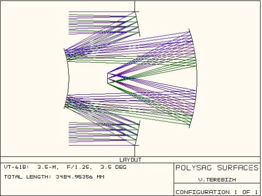
Figure 5: *

All-reflective 3.5-m telescope
with a flat field of view of $3^{\circ}.5$ in diameter.

3.5-m telescope based on polysag surfaces

A wider field of view can be attained by applying the polysag surfaces of higher order, or by scaling down the 8.4-m designs discussed above. As a third example, using the polysag type surfaces, we consider 3.5-m telescope with a flat $3^{\circ}.5$ field. This system is presented in Figs. 5 and 6; with performance values given in Table 3. As one can see, the 3.5-m design has nearly diffraction-limited image quality.

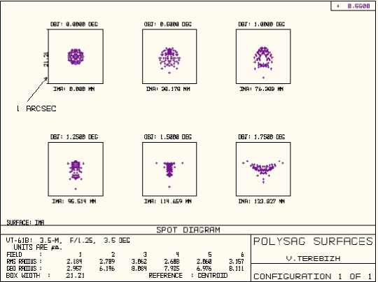
Figure 6: *

Spot diagrams of the telescope shown in Fig. 5
for the field angles $0,\,0^{\circ}.5,\,1^{\circ}.0,\,1^{\circ}.25,\,1^{\circ}.5$, and $1^{\circ}.75$.
Wavelength is $0.55\,\mu$m, the box width is $1^{\prime\prime}.0$ ($21.2\,\mu$m).

Concluding remarks

In practice, each of the telescopes considered above should be supplied with additional optical elements such as a filter and detector window. This, however, is not a simple problem at $f/\#\simeq 1.25$, because of longitudinal chromatic aberration (see Schroeder [2000] for the discussion and examples). Although a nearly afocal pair of filter and window lenses could be introduced with an acceptable loss of image quality, the design loses some advantages of the initial all-reflective telescope. Use of thin flat plates as the filter and window appears to be a preferable solution. For example, placing a plate 5 mm thick approximately 10 mm from the detector in the 8.4-m design results in image deterioration of roughly $20\%$. According to M. Ackermann (private communication), this approach is currently being studied at the Sandia National Laboratories.

For some kinds of observations, image distortion may be important. We did not specifically restrict distortion in the proposed designs. Its value of 0.087% for the first design can be reduced at least a factor of two with negligible loss of the image quality.

We choose the $3^{\circ}.0$ field mainly to facilitate comparison with other systems; perhaps, one can reach the wider field even for a 8.4-m aperture. As mentioned previously, scaling down the designs discussed above is a useful way for creating attractive telescopes with a wider field and simpler surfaces. Indeed, it is much easier to restrict aberrations and obscuration for smaller systems. Also, necessary components such as filters and windows can be added while still maintaining high image quality with the addition of a lens field corrector. This is allowable for the ground-based telescopes, but for the space systems the inherent advantage of the purely reflective optics cannot be matched.

The author is grateful to M.R. Ackermann and V.V. Biryukov for useful discussions.

Appendix:
The complete description of the designs

Table A1. First version of the 8.4-m telescopea
Number		Curvature	Thickness		Light
of the	Comments	radius	(mm)	Glass	diameter
surface		(mm)			(mm)
1	Shieldb	$\infty$	5121.208	—	3540.0
2	Aperture stopc	$\infty$	481.379	—	8400.0
3	Primaryd	$-20556.85$	$-5602.588$	Mirror	8400.0
4	Secondarye	$-26012.21$	$5602.588$	Mirror	3538.1
5	Beam on primaryf	$-20556.85$	$1465.335$	—	5500.0
6	Tertiaryg	$-8619.046$	$-5477.544$	Mirror	5900.0
7	Imageh	$\infty$			550.4

^a) All conic constants are equal to zero.
^b) Standard surface. Circular obscuration between radiuses 0.0 and 1770.0 mm.
^c) Standard surface.
^d) Even asphere surface with $\alpha_{1}=-3.001299e-006$, $\alpha_{2}=1.657118e-014$, and $\alpha_{3}=6.364267e-024$. Circular aperture between radiuses 2620.0 and 4200.0 mm.
^e) Even asphere surface with $\alpha_{1}=-6.349123e-005$, $\alpha_{2}=-5.017399e-013$, $\alpha_{3}=-2.061083e-020$, and $\alpha_{4}=-1.168727e-027$. Circular aperture between radiuses 0.0 and 1770.0 mm.
^f) Even asphere surface picked up from the primary mirror. Circular aperture between radiuses 0.0 and 2620.0 mm.
^g) Even asphere surface with $\alpha_{1}=3.283586e-006$, $\alpha_{2}=7.158976e-015$, and $\alpha_{3}=-1.745620e-022$. Circular aperture between radiuses 0.0 and 2950.0 mm.
^h Standard flat surface.

Table A2. Second version of the 8.4-m telescope
Number		Curvature	Thickness		Light	Conic
of the	Comments	radius	(mm)	Glass	diameter
surface		(mm)			(mm)
1	Shielda	$\infty$	5196.805	—	3600.0	0
2	Aperture stopb	$\infty$	476.775	—	8400.0	0
3	Primaryc	$-18481.55$	$-5673.58$	Mirror	8400.0	$-1.083191$
4	Secondaryd	$-6080.58$	$5673.58$	Mirror	3525.3	$-0.041400$
5	Beam
	on primarye	$-18481.55$	$1598.275$	—	5500.0	0
6	Tertiaryf	$-9165.65$	$-5485.393$	Mirror	5950.0	0.146856
7	Imageg	$\infty$			550.4	0

^a) Standard surface. Circular obscuration between radiuses 0.0 and 1800.0 mm.
^b) Standard surface.
^c) Polysag surface with $a_{3}=2.175935e-005$. Circular aperture between radiuses 2620.0 and 4200.0 mm.
^d) Polysag surface with $a_{3}=3.175638e-004$, $a_{4}=-9.861486e-008$. Circular aperture between radiuses 0.0 and 1770.0 mm.
^e) Polysag surface picked up from the primary mirror. Circular aperture between radiuses 0.0 and 2620.0 mm.
^f) Polysag surface with $a_{3}=1.265684e-005$. Circular aperture between radiuses 0.0 and 2975.0 mm.
^g Standard flat surface.

References

- [1] M.R. Ackermann, J.T. McGraw, P.C. Zimmer, 2006. Ground-based and Airborne Telescopes, ed. by L.M. Stepp., Proc. of SPIE, Vol. 6267, 626740.
- [2] J.R.P. Angel, M. Lesser, R. Sarlot, T. Dunham, 2000. ASP Conf. Ser. 195, 81.
- [3] J. Baker, 1969. IEEE Trans. Aerosp. Electron. Syst. 5, 261.
- [4] D. Korsch, 1972. Applied Optics 11, 2986.
- [5] D. Korsch, 1977. Applied Optics 16, 2074.
- [6] C. Lanczos, 1988. Applied Analysis, Dover, New York.
- [7] M.Mersenne, 1636. L’Harmonie Universelle: De la nature des sons, Paris.
- [8] M. Paul, 1935. Rev. Opt. Theor. Instrum. 14, 169.
-
[9]
W.H. Press, S.A. Teukolsky, W.T. Wetterling, B.P. Flannery,
1992.
Numerical Recipes, Cambridge. - [10] M.M. Rusinov, 1973. Non-spherical surfaces in optics, Nedra, Moscow (in Russian).
- [11] B. Schmidt, 1930. Mitteilungen Hamburger Sternwarte in Bergedorf 7(36), 15. Reprinted: Selected Papers on Astronomical Optics, D.J. Schroeder (ed.), SPIE Milestone Series 73, 165, 1993.
- [12] D. J. Schroeder, 2000. Astronomical Optics, Academic Press, San Diego.
- [13] K. Schwarzschild, 1905. Astronomische Mittheilungen der Koniglichen Sternwarte zu Gottingen 10, 3 (Part II). Reprinted: Selected Papers on Astronomical Optics, D.J. Schroeder (ed.), SPIE Milestone Series 73, 3, 1993.
- [14] L.G. Seppala, 2002. Proc. SPIE 4836-19.
-
[15]
V.Yu. Terebizh, 2005. Astron. Letters 2005, 31, 129;
ArXiv: astro-ph/0502121 5 Feb 2005. -
[16]
V.Yu. Terebizh, 2006. ArXiv: astro-ph/0605361 15 May 2006;
Astron. Reports 2007, 51, 597. - [17] R.V. Willstrop, 1984. MNRAS 210, 597.