Fuzzy communities and the concept of bridgeness in complex networks

Abstract

We consider the problem of fuzzy community detection in networks, which complements and expands the concept of overlapping community structure. Our approach allows each vertex of the graph to belong to multiple communities at the same time, determined by exact numerical membership degrees, even in the presence of uncertainty in the data being analyzed. We created an algorithm for determining the optimal membership degrees with respect to a given goal function. Based on the membership degrees, we introduce a new measure that is able to identify outlier vertices that do not belong to any of the communities, bridge vertices that belong significantly to more than one single community, and regular vertices that fundamentally restrict their interactions within their own community, while also being able to quantify the centrality of a vertex with respect to its dominant community. The method can also be used for prediction in case of uncertainty in the dataset analyzed. The number of communities can be given in advance, or determined by the algorithm itself using a fuzzified variant of the modularity function. The technique is able to discover the fuzzy community structure of different real world networks including, but not limited to social networks, scientific collaboration networks and cortical networks with high confidence.

I Introduction

Recent studies revealed that graph models of many real world phenomena exhibit an overlapping community structure, which is hard to grasp with the classical graph clustering methods where every vertex of the graph belongs to exactly one community Palla et al. (2005). This is especially true for social networks, where it is not uncommon that individuals in the network belong to more than one community at the same time. Individuals who connect groups in the network function as “bridges”, hence the concept of “bridge” is defined as the vertices that cross structural holes between discrete groups of people Burt (1992). It is therefore important to define a quantity that measures the commitment of a node to several communities in order to obtain a more realistic view of these networks.

The intuitive meaning of a bridge vertex may differ in different kinds of networks that exist beyond sociometrics. In protein interaction networks, bridges can be proteins with multiple roles. In cortical networks containing brain areas responsible for different modalities (for instance, visual and tactile input processing), the bridges are presumably the areas that take part in the integration and higher level processing of sensory signals. In word association networks, words with multiple meanings are likely to be bridges . The state-of-the-art overlapping community detection algorithms Reichardt and Bornholdt (2004); Palla et al. (2005); Capocci et al. (2005); Zhang et al. (2007) are not able to quantify the notion of bridgeness, while other attempts at quantifying it (e.g., the participation index Guimerà and Amaral (2005)) are only concerned with non-overlapping communities.

To emphasize the importance of bridge vertices in community detection and to illustrate the concept, we take a simple graph shown on Fig. 1(a) as an example. A visual inspection of this graph most likely suggests two densely connected communities, with vertex 5 standing somewhere in between, belonging to both of them at the same time. One may argue that vertex 5 itself forms a separate community, but a community with only a single node is usually not meaningful (and we can also easily add more edges connecting the two communities to vertex 5 to emphasize its sharedness). This property of vertex 5 is not revealed by any classical community detection algorithm without accounting for overlaps or outliers.

(a)  

(b)  

Figure 1: Panel $(a)$: a simple graph that is unable to be partitioned into two communities without allowing overlaps or outliers. Panel $(b)$: the dendrogram of the graph as calculated by the greedy modularity optimization algorithm Clauset et al. (2004). The dashed line denotes the level where the dendrogram should be cut in order to reach the maximal modularity (denoted by $q$).

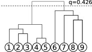
Hierarchical algorithms build a dendrogram from the vertices by joining them to communities one by one (or starting from the opposite direction, splitting the graph into two subcommunities, then splitting the subcommunities again until every vertex forms a single community). For instance, the modularity optimization algorithm of Clauset et al Clauset et al. (2004) repeatedly merges individual vertices or already created communities to form bigger ones in a way that greedily maximizes the modularity of the achieved partition (for the definition of modularity, see Newman (2004) or Eq. 13). Using this algorithm, vertex 5 was merged to vertex 4 right at the first step of the algorithm, misleadingly suggesting that they can not be separated from each other. The complete dendrogram is shown on Fig. 1(b).

A better solution can be achieved by applying the clique percolation method (CPM) of Palla et al Palla et al. (2005), which is also able to discover overlapping communities. In this case, vertex 5 was classified as an outlier (a vertex that does not belong to any community). This result stands closer to our visual inspection and clearly underlines the fact that in many cases, we should not assume that a vertex belongs to one and only one community in the graph. However, vertex 5 is not an outlier in the sense that removing it from the network would result in two disconnected components. Vertex 5 is an integral part of the network, serving as the only connection between two densely connected subgroups.

II Methods

II.1 Fuzzy community detection as a constrained optimization problem

The objective of classical community detection in networks is to partition the vertex set of the graph $G(V,E)$ into $c$ distinct subsets in a way that puts densely connected groups of vertices in the same community. $c$ can either be given in advance or determined by the community detection algorithm itself. For the time being, let us assume that $c$ is known. In this case, a convenient representation of a given partition is the partition matrix $\mathbf{U}=\left[u_{ik}\right]$ Bezdek (1981). $\mathbf{U}$ has $N=|V|$ columns and $c$ rows, and $u_{ik}=1$ if and only if vertex $k$ belongs to the $i$th subset in the partition, otherwise it is zero. From the definition of the partition, it clearly follows that $\sum_{i=1}^{c}u_{ik}=1$ for all $1\leq k\leq N$. The size of community $i$ can then be calculated as $\sum_{k=1}^{N}u_{ik}$, and for any meaningful partition, we can assume that $0<\sum_{k=1}^{N}u_{ik}<N$. These partitions are traditionally called hard or crisp partitions, because a vertex can belong to one and only one of the detected communities Bezdek (1981).

The generalization of the hard partition follows by allowing $u_{ik}$ to attain any real value from the interval $[0,1]$. The constraints imposed on the partition matrix remain the same Ruspini (1970):

$$u_{ik}\in[0,1]\mbox{\leavevmode\nobreak\ for all\leavevmode\nobreak\ }1\leq i\leq c,1\leq k\leq N$$ (1a)

$$\sum_{i=1}^{c}u_{ik}=1\mbox{\leavevmode\nobreak\ for all\leavevmode\nobreak\ }1\leq k\leq N$$ (1b)

$$0<\sum_{k=1}^{N}u_{ik}<N\mbox{\leavevmode\nobreak\ for all\leavevmode\nobreak\ }1\leq i\leq c.$$ (1c)

Eq. 1b simply states that the total membership degree for each vertex must be equal to 1. Informally, this means that vertices have a total membership degree of 1, which will be distributed among the communities. Eq. 1c is the formal description of a simple requirement: we are not interested in empty communities (to which no vertex belongs to any extent), and we do not want all vertices to be grouped into a single community. Partitions of this type are called fuzzy partitions. The fuzzy membership degrees for a given vertex can be thought about as a trait vector that describes some (possibly nonobservable) properties of the entity which the vertex represents in a compact manner. Trait-based graph models have already been suggested as models for complex networks Zalányi et al. (2003).

Since the groundbreaking work of Dunn Dunn (1973) and Bezdek Bezdek (1981) on the fuzzy $c$-means clustering algorithm, many methods have been developed to search for fuzzy clusters in multi-dimensional datasets. For an overview of these methods, see Bezdek and Pal Bezdek and Pal (1992). However, these methods usually require a distance function defined in the space the data belong to, therefore it is impossible to apply them to graph partitioning directly, except in cases where the vertices of the graph are embedded in an $n$-dimensional space. A recent paper of Zhang et al Zhang et al. (2007) discusses a possible embedding of the vertices of an arbitrary graph into an $n$-dimensional space using spectral mapping in order to utilize the fuzzy $c$-means algorithm on graphs. They were able to identify meaningful fuzzy communities in several well-known test graphs (e.g., the Zachary karate club network Zachary (1977) and the network of American college football teams Girvan and Newman (2002)), but the eigenvector calculations involved in the algorithm render it computationally expensive to use on large networks.

To overcome the need of spatial embedding, we propose a different approach based on vertex similarities. We observe that a meaningful partition (let it be hard or fuzzy) should group vertices that are somehow similar to each other in the same community. It is reasonable to assume that an edge between vertex $v_{1}$ and $v_{2}$ implies the similarity of $v_{1}$ and $v_{2}$, and likewise, the absence of an edge implies dissimilarity. Let us assume that we have a function $s(\mathbf{U},i,j)$ that satisfies the following criteria:

1. $s(\mathbf{U},i,j)\in[0,1]$

2. $s(\mathbf{U},i,j)$ is continuous and differentiable for all $u_{ij}$.

3. $s(\mathbf{U},i,j)=1$ if the membership values of $v_{i}$ and $v_{j}$ suggest that they are as similar as possible.

4. $s(\mathbf{U},i,j)=0$ if the membership values of $v_{i}$ and $v_{j}$ suggest that they are completely dissimilar (there is no chance that they belong to the same community).

Let us call such $s(\mathbf{U},i,j)$ a similarity function, and for the sake of simplicity, we simply denote it by $s_{ij}$ from now on (not emphasizing its dependence on $\mathbf{U}$). Suppose we have a prior assumption about the actual similarity of the vertices, denoted by $\tilde{s}_{ij}$ for $v_{i}$ and $v_{j}$. This leads us to the following equation, which measures the fitness of a given partition $\mathbf{U}$ of graph $G(V,E)$ by quantifying how precisely it approximates the prescribed similarity values with $s_{ij}$:

$$D_{G}(\mathbf{U})=\sum_{i=1}^{N}\sum_{j=1}^{N}w_{ij}\left(\tilde{s}_{ij}-s_{ij}\right)^{2},$$ (2)

where $w_{ij}$’s are optional weights and $N=|V|$ is the number of vertices in the graph. For the sake of notational simplicity, we also introduce the matrices $\mathbf{W}=\left[w_{ij}\right]$, $\mathbf{S}(\mathbf{U})=\left[s_{ij}\right]$ and $\mathbf{\tilde{S}}=\left[\tilde{s}_{ij}\right]$. From now on, we assume that $\mathbf{\tilde{S}}=\mathbf{A}_{G}$, the adjacency matrix of the graph, in concordance with our assumption that the similarity of connected vertex pairs should be close to 1 and the similarity of disconnected vertex pairs should be close to zero. The only thing left is to precisely define a similarity function $s_{ij}$ that satisfies the conditions prescribed above. The definition we used was the following:

$$s_{ij}=\sum_{k=1}^{c}u_{ki}u_{kj}$$ (3)

It easily follows that $\mathbf{S}(\mathbf{U})=\left[s_{ij}\right]=\mathbf{U}^{T}\mathbf{U}$ .

In summary, the community detection problem in this framework boils down to the optimization of $D_{G}(\mathbf{U})$ defined in Eq. 2: we must find $\mathbf{U}$ that minimizes $D_{G}(\mathbf{U})$ while satisfying the conditions of Eq. 1. The number of clusters $c$, the weight matrix $\mathbf{W}$ and the desired similarities $\mathbf{\tilde{S}}$ are given in advance (the latter one most commonly equals to the adjacency matrix $\mathbf{A}_{G}$). This is a nonlinear constrained optimization problem. Although there exist a set of necessary conditions that restrict the set of possible $\mathbf{U}$’s worth evaluating Karush (1939); Kuhn and Tucker (1951), the computationally most feasible approach to optimize $D_{G}(\mathbf{U})$ is to use a gradient-based iterative optimization method (e.g., simulated annealing). The equality constraints in Eq. 1b can be incorporated into the goal function by Lagrangian multipliers $\mathbf{\lambda}=\left[\lambda_{1},\lambda_{2},\dots\lambda_{N}\right]$, resulting in the following modified goal function:

$$\tilde{D}_{G}(\mathbf{U},\mathbf{\lambda}) =\displaystyle\sum_{i=1}^{N}\sum_{j=1}^{N}w_{ij}\left(\tilde{s}_{ij}-s_{ij}\right)^{2}+$$ (4)

$$\displaystyle\sum_{i=1}^{N}\lambda_{i}\left(\sum_{k=1}^{c}u_{ki}-1\right),$$

The modified goal function compactly encodes the original goal function and the constraints, since $\nabla_{u_{ij}}\tilde{D}_{G}(\mathbf{U},\mathbf{\lambda})=0$ (for all $1\leq i\leq c$ and $1\leq j\leq N$) ensures that we are at a stationary point of the goal function, and $\nabla_{\mathbf{\lambda}}\tilde{D}_{G}(\mathbf{U},\mathbf{\lambda})=0$ ensures that we satisfy the conditions of Eq. 1b. Therefore, stationary points of Eq. 4 will also be stationary points of Eq. 2 and they do not violate Eq. 1b.

To employ a gradient-based iterative optimization method, we need the derivatives of the goal function with respect to $u_{kl}$. First we note that

$$\frac{\partial s_{ij}}{\partial u_{kl}}=\frac{\partial}{\partial u_{kl}}\left(u_{ki}u_{kj}\right)$$ (5)

which is zero, except when $i=l$ or $j=l$:

$$\frac{\partial s_{ij}}{\partial u_{kl}}=\left\{\begin{array}[]{ll}2u_{kl}&\mbox{if\leavevmode\nobreak\ }i=l\wedge j=l\\ u_{ki}&\mbox{if\leavevmode\nobreak\ }i\neq l\wedge j=l\\ u_{kj}&\mbox{if\leavevmode\nobreak\ }i=l\wedge j\neq l\\ 0&\mbox{if\leavevmode\nobreak\ }i\neq l\wedge j\neq l\end{array}\right.$$ (6)

The partial derivative of $\tilde{D}_{G}(\mathbf{U},\mathbf{\lambda})$ with respect to $u_{kl}$ is therefore

$$\frac{\partial\tilde{D}_{G}}{\partial u_{kl}} = \displaystyle-2\sum_{i=1}^{N}w_{il}(\tilde{s}_{il}-s_{il})u_{ki}$$ (7)

$$\displaystyle-2\sum_{j=1}^{N}w_{lj}(\tilde{s}_{lj}-s_{lj})u_{kj}+\lambda_{l}$$

Let $e_{ij}=w_{ij}\left(\tilde{s}_{ij}-s_{ij}\right)$. Summing the partial derivatives for $k=1,2,\dots c$, making them equal to zero and substituting Eq. 1b back where appropriate leaves us with:

$$\lambda_{l} = \displaystyle\frac{2}{c}\sum_{i=1}^{N}(e_{il}+e_{li})$$ (8)

The substitution of Eq. 8 into Eq. 7 yields one component of the goal function’s gradient vector:

$$\frac{\partial\tilde{D}_{G}}{\partial u_{kl}} = 2\sum_{i=1}^{N}(e_{il}+e_{li})\left(\frac{1}{c}-u_{ki}\right)$$ (9)

The simplest gradient-based algorithm for finding a local minimum of $\tilde{D}_{G}$ is then the following:

1. Start from an arbitrary random partition $\mathbf{U}^{(0)}$ and let $t=0$.

2. Calculate the gradient vector of $\tilde{D}_{G}$ according to Eq. 9 and the current $\mathbf{U}^{(t)}$.

3. If $\max_{k,l}|\frac{\partial\tilde{D}_{G}}{\partial u_{kl}}|<\varepsilon$, stop the iteration and declare $\mathbf{U}^{(t)}$ a solution.

4. Otherwise, calculate the next partition in the iteration with the following equation:

   $$u_{ij}^{(t+1)}=u_{ij}^{(t)}+\alpha^{(t)}\frac{\partial\tilde{D}_{G}}{\partial u_{ij}}$$ (10)

   where $\alpha^{(t)}$ is a small step size constant chosen appropriately.

5. Increase $t$ and continue from step 2.

$\alpha^{(t)}$ can be determined by a line search towards the direction defined by the gradient vector, it can be adjusted iteratively according to some simulated annealing schedule (see Nourani and Andresen (1998) for a comparison of strategies), or it can be made adaptive from iteration to iteration by checking the difference of the values of the goal function in the last few steps: the step size can be increased if the value of the goal function decreased, and it must be decreased if the value of the goal function increased. We must also make sure that the procedure does not end up in a saddle point or a local maximum of $D_{G}(\mathbf{U})$ .

According to our simulations, the quality of the result is not affected by the initial membership degrees, but the speed of convergence is. In the extreme case, if we choose all $u_{ij}$ to be equal to $1/c$, all the gradients will be zero (see Eq. 9), therefore it is suggested to use a randomized initial partition matrix. The best results can be achieved by choosing the initial membership degrees from a uniform distribution while still satisfying the sum constraints. Uniformity with respect to the constraints is not straightforward to achieve. The intuitive approach is to choose a random number from the interval $[0,1]$ for every $u_{ij}$ and divide them with their respective column sums to satisfy Eq. 1b. However, this method is biased towards membership vectors describing vertices equally participating in every community. The proper way to sample from all possible membership vectors is to draw every vector from a Dirichlet distribution with order $c$ and $\mathbf{\alpha}=\left[1,1,\dots,1\right]$ where $\mathbf{\alpha}$ has $c$ coordinates. Such a distribution can be generated by drawing $c$ independent random samples from gamma distributions each with shape and scale parameters equal to 1, and dividing each variable with the sum of all of them Devroye (1986).

With $N$ vertices and $c$ communities, the time complexity of calculating the initial membership is $O(Nc)$, calculating the gradient vectors in each step is $O(N^{2}c)$, choosing the maximum gradient component for each vertex is $O(Nc)$ and calculating the next partition matrix is $O(Nc)$, assuming that the step size can be chosen in $O(1)$ (which is true for simulated annealing strategies or adaptive step sizes based on the decline of the goal function between subsequent steps). This results in an overall time complexity of $O(N^{2}ch)$, where $h$ is the number of steps necessary for the algorithm to terminate, meaning that the calculation time is expected to scale quadratically with the number of vertices if $N\gg c$, which is confirmed by our measurements. The time complexity of our implementation (Fig. 2) is slightly worse than that of spectral methods, where an almost linear time complexity can be achieved by, e.g., using the implicitly restarted Arnoldi method Lehoucq and Sorensen (1996) to compute some of the largest eigenvectors.

Figure 2: Running time of our algorithm as a function of the number of vertices in a graph with 4 communities. The hardware used for calculation was an 1.83 GHz Intel Core Duo MacBook. Fitting $f(x)=ax^{b}$ resulted in the parameters $a=2.3\times 10^{-5}\pm 1\times 10^{-6}$ and $b=1.968\pm 4.24\times 10^{-3}$ (standard deviation from the fitted curve = 2.583), confirming our reasoning on the quadratic running time of the algorithm.

For the sake of completeness, we show that $\mathbf{U}^{(t+1)}$ remains a partition matrix if $\mathbf{U}^{(t)}$ was a partition matrix. We recall that a partition matrix satisfies Eq. 1a and Eq. 1b. In the first step, we choose $\mathbf{U}^{(0)}$ that satisfies Eq. 1c. The persistence of Eq. 1a and Eq. 1c is straightforward if we always keep $\alpha^{(t)}$ low enough, so we only have to prove the persistence of Eq. 1b:

$$\sum_{i=1}^{c}u_{ik}^{(t+1)} = \sum_{i=1}^{c}u_{ik}^{(t)}+\sum_{i=1}^{c}\alpha^{(t)}\frac{\partial\tilde{D}_{G}}{\partial u_{ik}^{(t)}}$$ (11)

$$= 1+2\alpha^{(t)}\sum_{i=1}^{c}\sum_{j=1}^{N}(e_{jk}+e_{kj})\left(\frac{1}{c}-u_{ij}^{(t)}\right)$$

$$= 1+2\alpha^{(t)}\sum_{j=1}^{N}(e_{jk}+e_{kj})\left(1-\sum_{i=1}^{c}u_{ij}^{(t)}\right)$$

$$= 1$$

II.2 The concept of bridgeness

One of the advantages of fuzzy community detection is that it enables us to analyze to what extent a given vertex is shared among different communities. This measure is called bridgeness. Intuitively, a vertex that belongs to only one of the communities has zero bridgeness, while a vertex that belongs to all of the communities exactly to the same extent has a bridgeness of 1. We define the bridgeness of a vertex $v_{i}$ as the distance of its membership vector $\mathbf{u}_{i}=\left[u_{1i},u_{2i},\dots,u_{ci}\right]$ from the reference vector $\left[\frac{1}{c},\frac{1}{c},\dots,\frac{1}{c}\right]$ in the Euclidean vector norm , inverted and normalized to the interval $[0,1]$ as follows:

$$b_{i}=1-\sqrt{\frac{c}{c-1}\sum_{j=1}^{c}\left(u_{ji}-\frac{1}{c}\right)^{2}}$$ (12)

Note that $b_{i}$ attains its theoretical maximum when $v_{i}$ belongs to all of the communities exactly with the same membership degree, therefore it is possible that in this case, $v_{i}$ is more likely to be an outlier in the graph (a vertex belonging to none of the communities) rather than a bridge. To distinguish outliers and real bridges, one should also look at the centrality measures of the node: high centrality supports the assumption that the vertex is effectively a bridge, because despite its central role in the network, the algorithm was not able to assign it to a single community. Low centrality may mean that the algorithm strived to make the vertex dissimilar from almost all other vertices, therefore it made it belong to all the communities. The simplest measure that incorporates centrality and bridgeness score into a single number is simply defined as the product of the degree and the bridgeness of the node, and will be called degree-corrected bridgeness from now on. Other centrality measures (e.g. betweenness centrality, closeness centrality or eigenvector centrality) can also be used. More sophisticated centrality measures take into account that several networks contain vertices that have a crucial role but a relatively low degree (e.g. metabolic networks, as shown in Guimerà and Amaral (2005)). We also suggest to plot a chosen centrality measure versus the bridgeness score for each vertex to visually aid the selection of bridge vertices and outliers. An example of this kind of plot will be shown in Section IV on Fig. 9.

Bridgeness can either be used in benchmarks to assess how sensitive the algorithm is to structural overlaps, or in the analysis of real data to gain information about the roles of the vertices in the network. Vertices with high centrality and bridgeness scores close to zero are likely to be in the cores of the communities, while bridgeness scores close to one with a high centrality suggest vertices standing in a bridgelike position between communities. In this sense, substracting the bridgeness score from 1 and multiplying it by an appropriate centrality measure results in a measure of the centrality of the vertex with respect to its own communities in the network, similarly to the measure introduced in Newman (2006). Benchmark results and the application of bridgeness in data analysis is presented in Section IV.

III Parametrization of the algorithm

At first glance, it may seem difficult to select the appropriate value for each parameter of the algorithm described in the previous section. However, most of these parameters have reasonable default values that can be used in most cases. The only exception is the number of clusters $c$, for which we will describe a simple process to identify its most suitable value. In this section, we explain the key ideas one should consider when choosing the appropriate values for the parameters.

III.1 Choosing the number of communities

The first and most important parameter of the method is $c$, defining the number of communities the algorithm tries to discover in the network. This parameter is the keystone of most community detection algorithms, and determining $c$ in a self-consistent way without human intervention is definitely a complicated problem. Spectral methods rely on the largest eigenvalues of the adjacency matrix $\mathbf{A}_{G}$ or the smallest eigenvalues of the Laplacian matrix $\mathbf{L}_{G}=\mathbf{A}_{G}-\mathbf{D}_{G}$ (where $\mathbf{D}_{G}$ is a diagonal matrix with diagonal elements $k_{i}$, the degrees of the vertices) to define the number of communities, but this is usually done by visual inspection, and since the eigenspectrum of most networks found in real applications resemble a straight line instead of a step function, choosing $c$ is not free of subjective elements. For instance, the number of eigenvalues of the Laplacian matrix of a graph that are close to zero are often used as the value of $c$, but this only replaces the value of $c$ with another parameter: a threshold level that decides which eigenvalues are considered to be close to zero. The threshold is then chosen manually.

In order to get rid of the human intervention needed to choose $c$ based on the eigenvalues, we propose a different, divisive approach which also spares some computation in the early stage of the algorithm. Initially, we compute a fuzzy bisection of the graph by setting $c=2$. After that, whenever the optimization gets stuck in a local minimum, we add another degree of freedom to the system by increasing $c$ and continue with the optimization from the last local minimum until it converges again. We keep on increasing the number of communities until we find that the newly introduced community does not improve the overall community structure of the network (after the algorithm has settled down again in a minimum). The community structure is assessed by the fuzzification of the modularity function. The modularity, originally introduced in Newman (2004), defines how good a community structure is by evaluating the difference between the observed intra-community edge density and the expected one based on a random graph model conditioned on the degree sequence of the network. In a random graph with exactly the same degree sequence as the original graph, the probability of the existence of an edge between vertices $i$ and $j$ is $k_{i}k_{j}/2m$, where $k_{i}$ is the degree of vertex $i$ and $m$ is the total number of edges in the network. The original, “crisp” modularity of a network with vertex $i$ belonging to community $c(i)$ is then defined as:

$$Q=\frac{1}{2m}\sum_{i,j}\left[A_{ij}-\frac{k_{i}k_{j}}{2m}\right]\delta_{c(i),c(j)}$$ (13)

where $\delta_{c(i),c(j)}$ is 1 if vertex $i$ and $j$ belong to the same community ($c(i)=c(j)$), 0 otherwise. Since the community structure in our algorithm is not clear-cut, the following predicate: “vertex $i$ and $j$ belongs to the same community” also has a fuzzy truth value between 0 and 1. When the membership degree $u_{ki}$ is considered the probability of the event that vertex $i$ is in community $k$, the probability of the event that vertex $i$ belongs to the same community as vertex $j$ becomes the dot product of their membership vectors, resulting in the already introduced similarity measure $s_{ij}$, which can be used in place of $\delta_{c(i),c(j)}$ to obtain a fuzzified variant of the modularity:

$$Q_{f}=\frac{1}{2m}\sum_{i,j}\left[A_{ij}-\frac{k_{i}k_{j}}{2m}\right]s_{ij}$$ (14)

Note that in the case of crisp communities (there exists only one $k$ for every vertex $i$ such that $u_{ik}=1$), the fuzzified modularity $Q_{f}$ is exactly the same as the crisp modularity $Q$. In order to determine the optimal number of fuzzy communities, we iteratively increase $c$ and choose the one which results in the highest fuzzified modularity $Q_{f}$.

III.2 Parametrization of similarity and dissimilarity constraints

Next, we discuss the appropriate choice of the remaining parameters ($\mathbf{W}$ and $\mathbf{\tilde{S}}$). These parameters are not crucial to the final result of the algorithm, but they provide a way to inject additional a priori knowledge into the algorithm. Note that the goal function (see Eq. 2) is a weighted sum of the difference between the desired and the calculated similarity values. The algorithm tries to minimize the difference by fitting the membership values in an appropriate way. Without any further a priori knowledge, $\mathbf{\tilde{S}}$ is the adjacency matrix $\mathbf{A}_{G}$ and $\mathbf{W}$ is a matrix containing only ones. This means that the dot product of the membership vectors define the similarities, and the desired similarity is 1 for adjacent and 0 for nonadjacent vertices, stating that the endpoints of the edges should be as similar as possible, while keeping disconnected edges dissimilar. The latter requirement is important: if we would only specify that the endpoints should be similar for connected vertex pairs, the algorithm would converge to a state where every vertex belongs to the same community.

Depending on the domain from which the network being analyzed originates, there may be some additional knowledge about the original mechanism that created the network, or there may be some uncertainty in the data. $\mathbf{W}$ can be used to fine-tune the algorithm by making use of the domain-specific knowledge. The general purpose of $w_{ij}$ is to emphasize the connections where the calculated similarity should match the expected one and skip the connections where it is hard or impossible to specify an expected similarity. $w_{ij}$ can also be useful in the analysis of weighted networks.

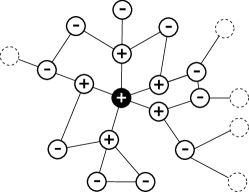
Consider a large friendship network as an example. In a friendship network, a reasonable assumption is that an existence of a connection between $A$ and $B$ predicts some kind of similarity between them. However, a missing connection between $A$ and $B$ does not necessarily mean dissimilarity, it might happen that $A$ and $B$ did not have a chance to meet and form a connection! To account for this, one can assume that $A$ is similar to its direct neighbors and dissimilar to its second order neighbors only (because they were likely to meet through their common acquaintances). If necessary, this assumption can be incorporated into Eq. 2 by setting the weight of the connections of $A$ beyond its second order neighbors to zero. We call this modification the distance-based relaxation of the model. For an illustration of the concept, see Fig. 3.

Figure 3: The idea of distance-based relaxation. Direct neighbors of vertex $i$ (denoted by plus signs) are assumed to be similar to vertex $i$ (shown in black): $\tilde{s}_{ij}=1,w_{ij}>0$. Vertices at most $k$ steps far from vertex $i$ that are not direct neighbors (denoted by minus signs) are assumed to be dissimilar: $\tilde{s}_{ij}=0,w_{ij}>0$. Vertices being farther than $k$ steps (denoted by dashed circles) have no similarity specification with respect to vertex $i$: $w_{ij}=0$. The figure illustrates the case of $k=2$.

The proper choice of $w_{ij}$ also allows us to analyze the community structure of networks with incomplete data. An example of this kind of a network is described in Négyessy et al. (2006). A graph model of the visuo-tactile cortex of the macaque monkey was built based on the neural connections of the brain areas already documented in the literature. However, there are actually two kinds of missing edges in this network: the absence of an edge between brain areas $A$ and $B$ can either mean that the specific connection was tested for experimentally and found to be nonexistent or that the connection has not ever been sought for at all (due to, e.g., methodological difficulties). Our model can account for this difference by setting the weight of the suspected connections to zero and checking the similarity of the vertices involved after the analysis. We will discuss this later in Section IV.

We also note that several other similarity measures can also be used when one defines the expected similarity matrix $\mathbf{\tilde{S}}$ as long as the similarities are normalized into the range $[0,1]$. Based only on the neighborhood of vertices, one can use the cosine similarity Salton and McGill (1983) or the Jaccard similarity index Jaccard (1901). More sophisticated, matrix-based methods have been studied in the papers of Jeh and Widom Jen and Widom (2002), Blondel et al Blondel et al. (2004) and Leicht et al Leicht et al. (2006). Some of these measures are not normalized to the range $[0,1]$, but this can be done easily by using an appropriate transformation (e.g., dividing the similarities by the largest one found in the network).

IV Benchmarks and applications

Generally, the community structure of a network is not uniquely defined. Several partitions might exist that approximate the underlying structure equally well, especially if the network exhibits an overlapping or hierarchical community structure. As shown in Palla et al. (2005), overlapping communities are present in many networks ranging from co-authorship networks to protein interactions. We expect our algorithm not only to discover this overlapping structure but also to exactly quantify the membership degree of each vertex in all of its communities.

Unless stated otherwise, we parametrized our algorithm as follows: $w_{ij}=1$ for all $i,j$ and the desired similarity $\tilde{s}_{ij}$ was 1 if vertices $i$ and $j$ were connected or $i$ was equal to $j$, 0 otherwise. The automatic selection of the bridges was achieved by the standardization of the bridgeness scores: a vertex was considered a bridge if its bridgeness score was at least one standard deviation higher than the mean bridgeness score of the vertices of the network.

IV.1 Benchmarks on computer-generated graphs

We tested our method on several computer-generated networks with nonoverlapping and overlapping community structure as well. Nonoverlapping community structures were generated on graphs with 1024 vertices grouped into four communities, each containing 256 vertices. Each vertex had an average of $k_{in}=24$ links to other vertices in the same community and an additional $k_{out}=8$ links to vertices from different communities. The generated graph had 16,384 edges and a density of 0.031. Overlapping communities were introduced by grouping the vertices into two communities and declaring 128 vertices in both communities as bridge vertices. Regular vertices kept their connectional patterns, having 24 links on average to other vertices in their community and 8 links to the other community. Bridge vertices had 6 links to other vertices in their community, 12 links to other bridge vertices in their community, 6 links to bridge vertices of the other community and 8 links to regular vertices of the other community. The edge count and the density was equal to the nonoverlapping case. Fig. 4 shows a possible adjacency matrix for both the nonoverlapping and the overlapping case.

Figure 4: Adjacency matrices of graphs with nonoverlapping (top) and overlapping (bottom) community structure we used for benchmarking our algorithm.

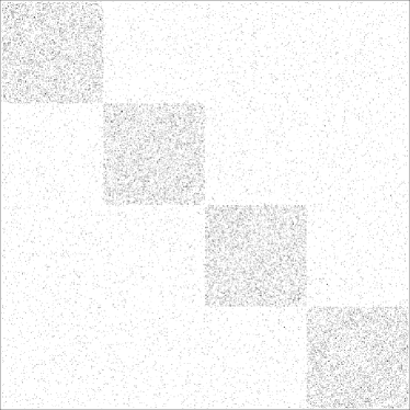
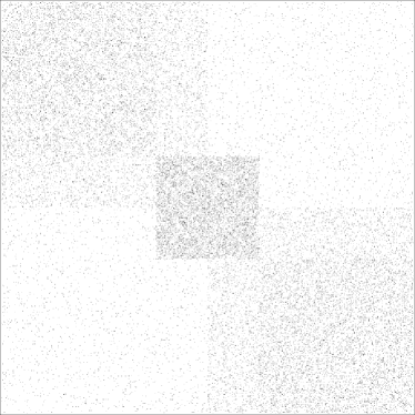
In order to compare a fuzzy partition with an expected hard partition, we introduced the notion of dominant community. The dominant community of a vertex is the community to which it belongs to the greatest extent. Formally, community $i$ is the dominant community of vertex $j$ if $u_{ij}\geq\max_{k}u_{kj}$ for $1\leq k\leq c$. Out of 1000 graphs with nonoverlapping community structures, the algorithm classified all vertices correctly in 97.4% of the test cases after converting the achieved fuzzy partition to its hard counterpart using the dominant communities. It was also able to infer the actual number of communities automatically in all cases using the fuzzified modularity. To further study the distribution of intra-community and inter-community edges, we varied the number of inter-community edges ($k_{out}$) from 0 to 24 while keeping $k_{in}+k_{out}$ constant. When $k_{out}$ reaches 24, the graph practically becomes an Erdős-Rényi random graph devoid of any community structure, since the connectional probability between any two of the pre-defined communities is equal. Fig. 5(a) shows the results of the benchmark. The quality of the calculated community structure was assessed by the normalized mutual information as described in Danon et al. (2005). Interestingly, the performance of the algorithm degrades suddenly when the number of inter-community links exceeds 16. This is the point where on average there are more links between the communities than inside them.

(a)  

(b)  

Figure 5: Panel $(a)$ shows the performance of the algorithm for a graph with nonoverlapping community structure. Inter-cluster link count ($k_{out}$) was varied while keeping the average degree ($k_{in}+k_{out}$) constant. The quality of the obtained result was measured using the normalized mutual information of the found and real communities Danon et al. (2005). Panel $(b)$ shows the frequencies of bridgeness values in a graph with overlapping community structure. Thin line shows frequencies for regular nodes, thick line shows frequencies for bridge nodes. The bin width of the histogram was set to 0.01 (100 bins).

Generated graphs with overlapping community structure were used to test the sensitivity of the algorithm to vertices standing between communities. The model we used declared 128 vertices out of 512 in both communities as bridge candidates, and clearly distinguished them by their different connectional patterns: bridge candidates tended to connect to each other with a higher probability than to the regular vertices in their communities, even if they originally belonged to different communities, creating an overlap between the two communities. Because of the randomized nature of this model, not all bridge candidates became real bridges between the communities, but they had a significantly higher chance of becoming one. We used the bridgeness value introduced in Section II.2 to assess the quality of the results. We expected that bridge candidate vertices exhibit a different bridgeness score distribution than the regular vertices in the same graph. We also required that vertices identified as bridges by our algorithm should be among those that have been declared bridge candidates before test graph generation. We generated 1000 random graphs using this graph model and plotted the distribution of the bridgeness scores on Fig. 5(b). The different nature of the two distributions was supported by a Kolmogorov-Smirnov test (p-value less than $2.2\times 10^{-16}$). Regular vertices usually had lower bridgeness scores than the bridge candidates, and we found that 92.8% of the identified bridges (based on their standardized bridgeness scores) were among bridge candidates, confirming that the algorithm is sensitive to the existence of overlaps between communities.

IV.2 Social and collaboration networks

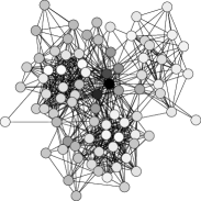
To evaluate the performance of our method on a real dataset, we used the social network of the academic staff of a given Faculty of a UK university consisting of three separate schools. The network structure was constructed from tie-strength measured with a questionnaire, where the items formed a reliable scale. Reliability was assessed by Cronbach’s $\alpha$ Cronbach (1951). Our questionnaire achieved a Cronbach’s $\alpha$ of 0.91, suggesting high internal consistency and reliability. The questionnaire was completed by every member of the academic staff. In this study, we used the personal friendship network, ignoring the directionality and the weight of the edges. A fuzzy community detection for three communities was performed on the graph. To show the results in grayscale, we decided to draw three individual figures (Fig. 6(a), 6(b) and 6(c)), showing the values of the membership functions for community 1, 2 and 3, respectively, using different shades of gray as fill colors for the vertices. Fig. 6(d) shows the degree-corrected bridgeness values for each vertex. Other centrality measures resulted in the same corrected bridgeness scores after normalization.

(a)  

(b)  

(c)  

(d)  

Figure 6: The fuzzy communities of the UK university faculty dataset. Panel (a), (b) and (c): vertices colored according to the membership functions of community 1, 2 and 3, respectively. Darker shades represent larger membership values. Panel (d): vertices colored according to the degree-corrected bridgeness scores. Darker shades represent higher bridgeness.

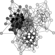
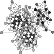
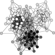
This dataset also contained explicit information regarding the expected community structure, since for every node, we knew which school in the Faculty does it belong to. We defuzzified the results using the dominant communities for every vertex. The defuzzification revealed that all crisp communities consisted of almost exclusively the members of a single school inside the Faculty. 75 out of 81 vertices were classified correctly, 4 were misclassified (and all of them had a bridgeness value greater than 0.7), and there were 2 vertices for which no expectation was given because of lack of information in the questionnaire. It is also noteworthy that the maximal fuzzy modularity ($Q_{f}$ = 0.2826) was reached at $c=6$, suggesting further subdivisions of the schools, although the improvement of the modularity compared to the case of $c=3$ ($Q_{f}$ = 0.2541) was not significant.

Degree-corrected bridgeness scores for $c=3$ (Fig. 6(d)) are particularly interesting. Highly scored individuals belong to all three communities at the same time to some extent, maintaining connections to all of them. On the other hand, vertices with low degree-corrected bridgeness scores can be thought as the cores of the communities. We also notice that the peripheries of the communities also belong almost equally to all of the communities (note the similar grey shades in Fig. 6(a), 6(b) and 6(c) for these vertices), but the degree-corrected bridgeness scores suppress this effect because of their low degree. The uncorrected and the degree-corrected scores are compared side-by-side on Fig. 7. We also point out that the uncorrected bridgeness scores can be used as a measure of the centrality of a given vertex with respect to its own dominant community by substracting it from 1.

(a)  

(b)  

Figure 7: Comparison of the uncorrected (left) and degree-corrected bridgeness scores (right) in the UK university dataset. Vertices are colored according to their respective bridgeness scores. Darker shades represent higher bridgeness scores. Note how the uncorrected bridgeness score correlates with the centrality of the vertices in their respective community.

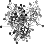
The next dataset we studied was the co-authorship network of scientists working on network theory and experiment, as published in Newman (2006). The network consists of 1589 scientist and 2742 weighted, undirected connections. Edge weights are derived from the number of joint publications: if author $A$ and $B$ share a paper where they are both authors and the paper has $n$ total authors, this contributes by $\frac{1}{n}$ to the total weight of the edge. We extracted the giant component of the network consisting of 379 scientists and 914 connections and let our algorithm determine the number of communities using the fuzzified modularity again. The optimum ($Q_{f}$ = 0.7082) was found with $c=30$ communities. The value of $c$ was confirmed by the visual inspection of the eigenvalues of the Laplacian matrix. Without names, we observe that vertices with the highest centralities according to our measure were similar to the ones chosen by the community centrality measure introduced in Newman (2006) and mostly represented senior researchers of the field of network science. Bridges were detected by standardizing the bridgeness values and considering vertices with a z-score higher than 1 as bridges. The 31 bridge vertices were mostly post-doctorate researchers who collaborated with more than one senior researcher of the field.

IV.3 Cortical networks and the case of incomplete data

To test how our method performs on graphs with missing data (vertex pairs for which no information regarding their connectedness was known), we used the graph model of the macaque monkey’s visuo-tactile cortex as published in Négyessy et al. (2006). The graph consists of 45 vertices representing brain areas, and 463 directed connections representing neuronal pathways between the areas. Disconnected vertices do not necessarily mean that there is no connection between them: some of them have been explicitly tested for and found to be absent, others have simply not been tested for (but generally thought to be absent), and there are 13 vertex pairs in total where neuroanatomists strongly suspect that there exists a connection between them. The graph itself consists of two distinct and mostly nonoverlapping communities corresponding to the visual and the somatosensory cortex. Other, anatomically meaningful subdivisions of the cortices (like the dorsal and the ventral stream in the visual cortex) are known as well. We also note that 11 out of the 13 suspected connections are heteromodal in the sense that they go between the visual and the somatosensory cortex.

To account for the uncertainty and the directedness of the edges in the graph, we specified $w_{ij}$ as follows: $w_{ij}$ was 0 if there was a nonreciprocal connection between area $i$ and $j$ (area $i$ connected to $j$, but no pathway was found in the reverse direction) or if the connection was one of the suspected ones, otherwise $w_{ij}$ was 1. The optimal fuzzy modularity (0.2766) was reached at $c=4$. We examined the results for $c=2$ and $c=4$. The case of $c=2$ classified the nodes correctly: all of the somatosensory areas were associated with the somatosensory cortex and most of the visual areas were associated with the visual cortex, except a few areas with a surprisingly high bridgeness (over 0.85). The vertex with the highest bridgeness (0.99) was area $46$, a part of the dorsolateral prefrontal cortex, and it does not have functions related to low-level sensory information processing. Area 46 is rather a higher level (supramodal) area, which plays a role in sustaining attention and working memory, and being a bridge between the visual and the somatosensory cortex, it integrates visual, tactile and other information necessary for the above mentioned cognitive functions. Other relevant bridges found with $c=4$ were area $VIP$ (where the literature has already suggested that it should be split into two areas $VIPm$ and $VIPp$, which establish stronger connections with visual or sensorimotor areas, respectively Lewis and Van Essen (2000)), $LIP$, $V4$ and $7a$. $VIP$ and $LIP$ are involved with hand and eye coordination, respectively, and both of these functions require combined information from visual and tactile signals as well. Area $7a$ integrates visual, tactile and proprioceptive signals. Area $V4$ was defined originally as the human color center Lueck et al. (1989); McKeefry and Zeki (1997), while it was also suggested that a separated ensemble of $V4$ neurons successfully encode complex shapes based on the curvature of the shape boundaries Pasupathy (2006). The functional heterogenity is in accordance to the subdivision of $V4$ into different regions as suggested by Bartels et al Bartels and Zeki (2000). We conclude that the bridges we found are in concordance with the assumed higher level roles of these areas. Fuzzy community detection for $c=4$ was also able to separate the dorsal and the ventral stream of the visual cortex, only area $7a$ and $VIP$ were misclassified, but they retained their bridgelike properties as well as area $46$. The degree-corrected bridgeness values for $c=4$ are shown on Fig. 8. Plotting the uncorrected bridgeness values versus a chosen centrality measure (in our case, the vertex degree), shown on Fig. 9 was found to be a useful visual aid for separating bridge vertices and outliers.

Figure 8: The cortical network dataset Négyessy et al. (2006). Rectangular vertices are visual areas, circular vertices are somatosensory areas. Vertices are colored according to their degree-corrected bridgeness values for $c=4$. Detected bridges are highlighted with white text color.

Figure 9: The degree-bridgeness plot of the vertices of the cortical network dataset for $c=4$. Crosses denote regular vertices and triangles denote bridges. Bridges and the single significant outlier (area $VOT$) have also been marked with the name of the corresponding area. The remaining names were omitted for sake of clarity. $VOT$ is a biologically relevant example of a vertex with low degree and high bridgeness.

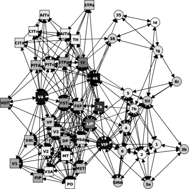
To approximate the probability of the suspected connections, we calculated the pairwise similarities of the vertices involved and considered the similarity as the probability of the existence of a connection. This is based on the idea that one can consider the membership value $u_{ij}$ as the probability of vertex $j$ belonging to community $i$. In this sense, the similarity of vertices $i$ and $j$ is the probability of the event that they are in the same community, and according to our prior assumption that similarity implies connectivity, we can think about higher similarity values as precursors for existing connections. Without going into further details and possible neuroanatomical implications, we concluded that all supposed connections of area $LIP$ are less likely than the supposed connections of $VIP$, and among the possible unknown connections of $VIP$, the connections with areas $4$ and $6$ are the most probable.

IV.4 Comparison with other overlapping community detection algorithms

In order to compare our method with earlier attempts on tackling the problem of overlapping communities, we examined the CPM algorithm of Palla et al Palla et al. (2005), the spectral method of Capocci et al Capocci et al. (2005) and the fuzzy method of Zhang et al Zhang et al. (2007). We tested all three methods on the example graph shown on Fig. 1(a) and on the macaque monkey dataset introduced in Section IV.3. For the CPM algorithm, we used the original implementation published by the authors at http://www.cfinder.org. The algorithm of Zhang et al had a weight exponent $m$ controlling the degree of fuzzification, but since the authors provided no clue about the suggested value of the parameter, we used $m=2$, which is the most typical choice of this parameter in other known applications of the fuzzy $c$-means algorithm Bezdek (1981).

The proper community structure of the example graph was detected by all algorithms we considered (including ours), although the spectral method of Capocci et al had to be tested on a different example graph with three cliques (each of size 4) and a single connector node, because in the case of only two communities, the only eigenvector that carries useful information is the first nontrivial one, rendering correlation calculations meaningless. Moreover, the global community structure became evident only after proper rearrangement of the community closeness matrix provided the algorithm. The bridge-like property of the connector vertex was inferred from the zero community closeness values to all other vertices. The method of Zhang et al and our method produced the proper expected partition matrix with all the vertices except vertex 5 classified strictly to one community or the other, while vertex 5 belonging to both at the same time with a membership degree of 0.5. The method of Palla et al identified vertex 5 as an outlier vertex, but after adding more edges to it, it became an overlap between the communities.

The community structure of the cortical graph seemed to be a harder problem for the algorithms. The method of Palla et al failed to discover the subdivision of the two main communities, only the visual and the somatosensory cortex was discovered when we used a clique size of 5. Larger clique sizes resulted in the discovery of the cores of the two communities, but we were not able to recognize the subdivision of the dorsal and the ventral stream in the visual cortex. However, the algorithm identified three overlaps ($V4$, $PITv$ and $TF$) for a clique size of 5 and two other overlaps ($LIP$ and $VIP$) for a clique size of 6. Three out of these five overlaps were identified by our algorithm as well. The community closeness matrix calculated by the method of Capocci et al was harder to interpret, but vertices $V4$ and $46$ clearly turned out to be bridges with zero community closenesses to many other vertices. The method of Zhang et al was highly sensitive on the exact value of parameter $m$, classifying 40% of the vertices as bridges for $m=2$. (Since the method provides a membership matrix similar to ours, we used the standardized bridgeness measure with a z-score threshold of 1). Lowering the weight exponent to $m=1.3$ identified vertices $LIP$, $7a$ and $Ri$ as bridges.

We found that the results of our algorithm with respect to community structure discovery and bridge identification do not contradict the results of existing methods, and all the bridges found by our algorithm were classified as bridges by at least one different method. The method of Capocci et al complements our algorithm especially well, since it discovers local communities around a given vertex using the community closeness degrees while our method provides useful insights into the global structure of the network being analyzed, also indicating the presence of bridge vertices.

V Conclusion

In this paper, we presented a fuzzy extension of classical community detection algorithms based on the assumption that communities of complex networks are formed by vertices with graded commitments towards at least one community. Accordingly, every vertex is allowed to belong to multiple communities with different membership degrees, represented by a single real value $u_{ki}\in\left[0,1\right]$ for each vertex $i$ and community $k$. The $\mathbf{U}=\left[u_{ki}\right]$ matrix encodes the membership values in a compact form and allows us to define the similarities of the vertices as $\mathbf{S}=\mathbf{U}^{T}\mathbf{U}$ in its simplest form. The similarities are then optimized using gradient-based constrained optimization methods in order to make connected vertices similar and disconnected vertices dissimilar. Based on the results of the fuzzy community detection, we introduced a novel concept called bridgeness, which can be used to measure to what extent is a given vertex shared between the communities. Vertices with high bridgeness values were shown to be important in various complex networks, including (but not limited to) social networks, scientific collaboration networks and cortical networks. A transformed variant of bridgeness can be used as a centrality measure with respect to the dominant communities of a vertex.

We emphasize that this algorithm is expected to be highly useful in the analysis of relatively small datasets (up to the magnitude of a thousand vertices). The reason is that the algorithm assumes that every vertex has the possibility to connect to all other vertices, and if they do not connect, they do that because they are of no use to each other. In very large networks, this assumption is not always realistic. However, the distance-based relaxation introduced in Section III can still be used in these cases to account for the upper bound imposed on the distance of the potentially interacting vertices.