Random-phase-approximation-based correlation energy functionals: Benchmark results for atoms

Abstract

The random phase approximation (RPA) for the correlation energy functional of density functional theory has recently attracted renewed interest. Formulated in terms of the Kohn-Sham (KS) orbitals and eigenvalues, it promises to resolve some of the fundamental limitations of the local density and generalized gradient approximations, as for instance their inability to account for dispersion forces. First results for atoms, however, indicate that the RPA overestimates correlation effects as much as the orbital-dependent functional obtained by a second order perturbation expansion on the basis of the KS Hamiltonian. In this contribution, three simple extensions of the RPA are examined, (a) its augmentation by an LDA for short-range correlation, (b) its combination with the second order exchange term, and (c) its combination with a partial resummation of the perturbation series including the second order exchange. It is found that the ground state and correlation energies as well as the ionization potentials resulting from the extensions (a) and (c) for closed sub-shell atoms are clearly superior to those obtained with the unmodified RPA. Quite some effort is made to ensure highly converged RPA data, so that the results may serve as benchmark data. The numerical techniques developed in this context, in particular for the inherent frequency integration, should also be useful for applications of RPA-type functionals to more complex systems.

I Introduction

Recent years have seen a revival of interest in the random phase approximation (RPA) and its extensions, both in the framework of Kohn-Sham density functional theory (KS-DFT) Dobson (1994); Pitarke and Eguiluz (1998); Dobson and Wang (1999); Kurth and Perdew (1999); Lein et al. (1999); Yan et al. (2000); Lein et al. (2000); Dobson and Wang (2000); Furche (2001); Fuchs and Gonze (2002); Miyake et al. (2002); Fuchs et al. (2003); Pitarke and Perdew (2003); Jung et al. (2004); Furche and Voorhis (2005); Fuchs et al. (2005); Marini et al. (2006) and within Green’s function-based many-body theory for ground state properties.Sánchez-Friera and Godby (2000); Garcia-Gonzalez and Godby (2002); Aryasetiawan et al. (2002); Dahlen and von Barth (2004); Dahlen et al. (2006) Within KS-DFT, the RPA for the energy and response function of the homogeneous electron gas played an important role in the development of the local-density approximation (LDA) as well as the generalized gradient approximation (GGA) for the exchange-correlation (XC) energy functional $E_{xc}$.Parr and Yang (1989); Dreizler and Gross (1990) Current interest in the RPA is stimulated by the concept of orbital-dependent (implicit) XC functionals, in which the XC energy is represented in terms of the KS orbitals and eigenenergies.Engel and Dreizler (1999); Grabo et al. (1999); Engel (2003); Görling (2005); Baerends (2005) Within this approach an RPA-type correlation energy functional is most easily formulated on the basis of the KS response function. Compared to LDA/GGA-type explicit XC functionals, implicit functionals have several attractive features: (1) the exchange can be treated exactly, leading to exchange energies and potentials which are free of self-interaction;Talman and Shadwick (1976) (2) the long-range dispersion interaction can be correctly described; Dobson (1994); Engel et al. (1998, 2000); Marini et al. (2006) (3) static correlation effects can be incorporated even within a spin-unpolarized formalism.Fuchs et al. (2003)

A systematic formulation of orbital-dependent XC functionals is possible within KS-based many-body theory, i.e.  by using the KS Hamiltonian as non-interacting reference Hamiltonian in the framework of standard many-body theory (KS-MBT).Sham (1985); Görling and Levy (1994); Engel (2003) In this approach the exact exchange of DFT emerges as first order contribution to a straightforward perturbation expansion in powers of $e^{2}$. All higher order terms constitute the DFT correlation energy. The lowest order correlation contribution resulting from perturbation theory, $E_{c}^{(2)}$, has been extensively studied for atoms and small molecules.Engel et al. (1998, 2000); Facco Bonetti et al. (2001); Grabowski et al. (2002); Mori-Sanchez et al. (2005); Jiang and Engel (2005) $E_{c}^{(2)}$ correctly accounts for the dispersion interaction Engel et al. (1998, 2000) and the corresponding correlation potential $v_{c}^{(2)}$ reproduces the shell-structure and asymptotic behavior of atomic correlation potentials.Jiang and Engel (2005) On the other hand, the magnitude of the energies and potentials resulting from $E_{c}^{(2)}$ overestimates the corresponding exact data significantly. Moreover, $E_{c}^{(2)}$ is found to be variationally instable for systems with a very small energy gap between the highest occupied and the lowest unoccupied molecular orbital (HOMO-LUMO gap) Jiang and Engel (2005); Mori-Sanchez et al. (2005) (as, for instance, the beryllium atom) and fails to describe chemical bonding in such elementary molecules as the nitrogen dimer.Engel (2003) The variational instability of $E_{c}^{(2)}$ can be resolved by resummation of suitable higher order contributions to infinite order (e.g.  in the form of Feynman diagrams). The simplest functional of this type is obtained by resummation of selected ladder-type diagrams, i.e.  the Epstein-Nesbet(EN)-diagrams. The resulting functional is not only found to be variationally stable for all neutral and singly-ionized atoms, but also gives more accurate correlation energies and potentials than $E_{c}^{(2)}$.Jiang and Engel (2006) However, EN-type functionals still face fundamental problems in the case of degenerate or near-degenerate systems. A more suitable partial resummation scheme is needed to establish a universally applicable, implicit XC functional, the RPA and its extensions being the prime candidates.

In standard many-body theory, the RPA is obtained by resummation of the so-called ring diagrams.Fetter and Walecka (1971) This concept can be directly transfered to the framework of KS-MBT.Engel and Facco Bonetti (2001) On the other hand, in the context of DFT, the RPA can also be derived from the adiabatic connection fluctuation-dissipation (ACFD) theorem.Langreth and Perdew (1977) The ACFD formalism is, for instance, the conceptual starting point for the recent development of van-der-Waals DFT.Dobson (1994) It has also been applied directly to various systems, including jellium surfaces and slabs,Dobson and Wang (1999), atoms Dahlen and von Barth (2004); Hellgren and von Barth (2007), small molecules Furche (2001); Fuchs and Gonze (2002); Furche and Voorhis (2005); Dahlen et al. (2006) and solids.Miyake et al. (2002); Marini et al. (2006) All these calculations have demonstrated promising features of RPA-based functionals. On the other hand, the results for atoms,Dahlen and von Barth (2004); Hellgren and von Barth (2007) for which rigorous benchmark data are available, indicate that the pure RPA overestimates correlation energies and potentials as much as $E_{c}^{(2)}$.

One is therefore led to consider extensions of the RPA. The most obvious starting point for extension is the inclusion of the second order exchange (SOX) contribution. However, in its pure form it neglects the screeening of the Coulomb interaction, which is the core feature of the RPA. One would thus expect an imbalance between direct and exchange contributions, when combining the RPA with the pure SOX term. A fully screened form of the SOX is easily formulated, following the line of thought used for the derivation of GGAs.Hu and Langreth (1986) The resulting functional, however, is computationally much more demanding than the RPA. For that reason it is worthwhile to examine alternative modifications of the SOX term which reduce its net contribution. Given the success of the EN-resummation in the context of the complete $E_{c}^{(2)}$, an EN-extension of the SOX term suggests itself (this functional is denoted as RSOX in the following).

The SOX term, be it screened or not, is inherently a short-range contribution. This raises the question whether it is sufficient to account for the complete screened SOX in an approximate fashion, relying on the LDA. In fact, using this strategy, one can easily include all short-range correlation effects beyond the RPA.Kurth and Perdew (1999); Yan et al. (2000) Clearly, the resulting LDA-type functional (here labelled as RPA+) is even more efficient than the RSOX.

In this work, we study the RPA and these simple extensions for a series of prototype atoms and ions, for which highly accurate reference data are available for comparison. In order to provide benchmark results a numerically exact, i.e. basis-set-free, approach is used and considerable emphasis is placed on all convergence issues involved. As a byproduct of this strive for accuracy, a highly efficient scheme for performing the frequency integration inherent in all RPA-type functionals has been developed. This procedure should be useful for applications to more complex systems, for which utilizing more than the minimum number of grid points for the frequency integration would be too demanding.

A complete implementation of any XC functional requires not only the evaluation of the XC energy, but also the inclusion of the corresponding XC potential $v_{\mathrm{xc}}$ in the self-consistent calculation. The latter step is quite challenging in the case of orbital-dependent XC functionals, for which $v_{\mathrm{xc}}$ has to be determined indirectly via the Optimized Potential Method (OPM),Talman and Shadwick (1976); Engel and Dreizler (1999); Grabo et al. (1999); Engel (2003); Görling (2005) and, in particular, for RPA-type functionals.Godby et al. (1987); Kotani (1998); Facco Bonetti et al. (2001, 2003); Niquet et al. (2003a, b); Jiang and Engel (2005); Grüning et al. (2006) Recently, Hellgren and von Barth have reported the first self-consistent RPA correlation potentials for spherical atoms, obtained by solution of the linearized Sham-Schluter equation Sham and Schlüter (1983) at the GW level.Hellgren and von Barth (2007) However, as indicated earlier, the RPA is not consistently improving atomic correlation potentials over $E_{c}^{(2)}$. In the present work we therefore focus on the perturbative evaluation of all RPA-type energies, utilizing self-consistent exchange-only orbitals and eigenvalues. As we will show, the RPA correlation energy is rather insensitive to the KS orbitals used for its evaluation, which clearly supports this perturbative approach. This feature, if true in general, will be very important for the application of RPA-type functionals to more complicated systems, for which a self-consistent implementation is not feasible anyway.

The paper is organized as follows. In the Section II, first the RPA correlation energy is formulated in the framework of the ACFD formalism. In addition, the general result is reduced to an expression valid for spherical systems. In Section III, various numerical aspects are discussed, addressing in particular questions of accuracy. In Section IV, the RPA correlation energies for a number of prototype atoms and ions (we will no longer distinguish between neutral atoms and atomic ions in the following) are presented and compared to the corresponding exact data. Section V provides a summary. Atomic units are used throughout this paper.

II Theory

II.1 RPA correlation energy on basis of the ACFD formalism

Based on the adiabatic connection and the zero-temperature fluctuation-dissipation theorem, Langreth and Perdew (1975, 1977) the exact KS correlation energy can be written as

$$E_{\rm c} = -\frac{1}{2\pi}\int_{0}^{\infty}du\int_{0}^{1}d\lambda\int d\mathbf{r}d\mathbf{r}^{\prime}v_{\mathrm{ee}}(\mathbf{r}-\mathbf{r}^{\prime})$$ (1)

$$\times\left[\chi_{\lambda}(\mathbf{r},\mathbf{r}^{\prime};iu)-\chi_{0}(\mathbf{r},\mathbf{r}^{\prime};iu)\right]\;,$$

where $v_{\mathrm{ee}}(\mathbf{r},\mathbf{r}^{\prime})=1/|\mathbf{r}-\mathbf{r}^{\prime}|$ is the bare Coulomb interaction, $\chi_{0}$ is the KS response function,

$$\chi_{0}(\mathbf{r},\mathbf{r}^{\prime};iu)=\sum_{ia}\frac{\phi_{i}^{\dagger}(\mathbf{r})\phi_{a}(\mathbf{r})\phi_{a}^{\dagger}(\mathbf{r}^{\prime})\phi_{i}(\mathbf{r}^{\prime})}{iu+\varepsilon_{i}-\varepsilon_{a}}+c.c.,$$ (2)

and $\chi_{\lambda}$, with $\lambda\in[0,1]$, is the density-density response function of a fictitious system in which electrons interact with a scaled Coulomb potential $\lambda v_{\mathrm{ee}}(\mathbf{r},\mathbf{r}^{\prime})$, and simultaneously move in a modified external potential, chosen such that the electron density remains identical to that of the fully interacting system with $\lambda=1$. Throughout this paper we use the convention that $i,j,\dots$ denote occupied (hole) KS states, while $a,b,\dots$ are used for unoccupied (particle) states and $p,q,\dots$ for the general case. $\chi_{\lambda}$ is related to $\chi_{0}$ by a Dyson-like integral equation, Gross and Kohn (1985)

$$\chi_{\lambda}(\mathbf{r},\mathbf{r}^{\prime},iu)=\chi_{0}(\mathbf{r},\mathbf{r}^{\prime},iu)+\int d\mathbf{r}_{1}\int d\mathbf{r}_{2}\chi_{0}(\mathbf{r},\mathbf{r}_{1},iu)K_{\lambda}(\mathbf{r}_{1},\mathbf{r}_{2},iu)\chi_{\lambda}(\mathbf{r}_{2},\mathbf{r}^{\prime},iu)\;,$$ (3)

where

$$K_{\lambda}(\mathbf{r}_{1},\mathbf{r}_{2},iu)=\lambda v_{\mathrm{ee}}(\mathbf{r}_{1},\mathbf{r}_{2})+f_{\mathrm{xc}}^{\lambda}(\mathbf{r}_{1},\mathbf{r}_{2},iu)$$ (4)

is the Coulomb and XC kernel.

The RPA correlation energy is obtained from Eq.(1) if one neglects the XC contribution to the right-hand side of Eq.(3). Integrating over $\lambda$ one ends up with

$$E_{\mathrm{c}}^{\mathrm{RPA}}=\int_{0}^{\infty}\frac{du}{2\pi}\mathrm{Tr}\left\{\mathrm{Ln}\left(1-\chi_{0}(iu)v_{\mathrm{ee}}\right)+\chi_{0}(iu)v_{\mathrm{ee}}\right\}\;,$$ (5)

where the trace indicates integration over all spatial coordinates. It is often more instructive to rewrite the integrand in Eq. (5), denoted as $E_{c}(iu)$, as a power series in the Coulomb interaction,

$$E_{c}(iu)=-\sum_{n=2}^{\infty}\mathrm{Tr}\left\{(\chi_{0}(iu)v_{\mathrm{ee}})^{n}\right\}\;.$$ (6)

II.2 Correlation energy beyond RPA

The ACFD theorem provides a natural starting point for the development of correlation functionals beyond the RPA: Inclusion of some approximation for $f_{xc}$ in the Dyson equation (3) automatically yields an extension of the RPA. Several approximate XC kernels have been introduced in the context of time-dependent DFT (TDDFT).Gross et al. (1996); Onida et al. (2002) It is, however, not clear whether an approximate $f_{xc}$ designed to provide a good description of excited states within TDDFT also leads to accurate ground state correlation energies.

A more straightforward extension of the RPA, the so-called RPA+ approach, had been proposed by Perdew and coworkers.Kurth and Perdew (1999); Yan et al. (2000) They observed that the RPA provides a quite accurate description of long-range correlation, but is inadequate for short-range correlations. On the other hand, the latter can be very well approximated by a local or semi-local density-based functional (LDA- or GGA-type),

$$E_{c}^{\mathrm{RPA+}}=E_{\mathrm{c,sr}}^{\mathrm{LDA}}+E_{\mathrm{c}}^{\mathrm{RPA}}$$ (7)

where the LDA for the short-range contribution $E_{\mathrm{c,sr}}$ can be obtained by subtraction of the RPA-limit from the full LDA correlation energy,

$$E_{\mathrm{c,sr}}^{\mathrm{LDA}}=E_{\mathrm{c}}^{\mathrm{LDA}}-E_{\mathrm{c}}^{\mathrm{LDA-RPA}}\;.$$ (8)

This approach is supported by the fact that the gradient correction to the short-range correlation is much smaller than that to the complete correlation energy.Kurth and Perdew (1999) Though the RPA+ functional has been used recently to describe the inter-layer dispersion interaction in boron nitride,Marini et al. (2006) a direct comparison of the RPA+ with exact results is still missing even for closed-shell atoms. Using numerically exact RPA correlation energy available for atoms, we are able to give a unambiguous assessment of the quality of the RPA+ correlation functional.

In the language of Feynman diagrams, the RPA correlation energy is obtained from the second order direct diagram by replacing the bare Coulomb interaction by the dynamically screened Coulomb interaction. The dominant contribution that is missing in the RPA is the second order exchange diagram (SOX),

$$E_{c}^{\mathrm{SOX}}=-\frac{1}{2}\sum_{ij,ab}\frac{\left(ij\mid\mid ab\right)\left(ab\mid\mid ji\right)}{\varepsilon_{i}+\varepsilon_{j}-\varepsilon_{a}-\varepsilon_{b}}\;,$$ (9)

where the notation

$$(pq||rs)=\int d^{3}r\int d^{3}r^{\prime}\,\frac{\phi_{p}^{\dagger}(\bm{r})\phi_{r}(\bm{r})\phi_{q}^{\dagger}(\bm{r}^{\prime})\phi_{s}(\bm{r}^{\prime})}{|\bm{r}-\bm{r}^{\prime}|}$$ (10)

has been used for the KS Slater integral. Combining the RPA with the SOX term, one obtains a new functional, denoted as RPA+SOX. However, one would expect the SOX to over-correct the error in the RPA, since the Coulomb interaction enters the SOX term in its bare, i.e.  un-screened, form. Screening can be introduced into the SOX term in a systematic way by use of the same, dynamically screened interaction as in the direct term. Hu and Langreth (1986) Unfortunately, the resulting functional is computationally much more demanding than the RPA expression. A technically much simpler way to reduce the SOX contribution has been suggested in the context of the second order functional $E_{c}^{(2)}$:Jiang and Engel (2006); Engel and Jiang (2006) The inclusion of the direct hole-hole contribution to the Epstein-Nesbet-type ladder diagrams into the SOX term substantially improves second order energies and potentials, without introducing any additional computational effort. Although the physical background of these ladder diagrams is quite different from dynamical screening, it seems worthwhile to analyze this “effective” screening. The resulting correction will be denoted as RSOX,

$$E_{c}^{\mathrm{RSOX}}=-\frac{1}{2}\sum_{i,j,a,b}\frac{\left(ij\mid\mid ab\right)\left(ab\mid\mid ji\right)}{\varepsilon_{i}+\varepsilon_{j}-\varepsilon_{a}-\varepsilon_{b}-\left(ij\mid\mid ij\right)}\;.$$ (11)

II.3 RPA correlation functional for spherical systems

In the case of spherical systems, the KS potential only depends on the radial coordinate $r$, $v_{\mathrm{s}}(\mathbf{r})=v_{\mathrm{s}}(r)$, and each KS orbital can be written as the product of a radial orbital and a spherical harmonic $Y_{lm}(\theta,\varphi)$,

$$\phi_{k}(\mathbf{r})\rightarrow\phi_{nlm}(\mathbf{r})=\frac{P_{nl}(r)}{r}Y_{lm}(\theta,\varphi),\;,$$ (12)

where $n$, $l$ and $m$ are the principle, angular and magnetic quantum numbers, respectively. The $P_{nl}$ are solutions of the radial KS equation,

$$\left[-\frac{1}{2}\left(\frac{d^{2}}{dr^{2}}-\frac{l(l+1)}{r^{2}}\right)+v_{\mathrm{s}}(r)\right]P_{nl}(r)=\varepsilon_{nl}P_{nl}(r)\;.$$ (13)

Two-body functions like the Coulomb interaction and $\chi_{0}$ can also be decomposed according to the spherical symmetry. To simplify notations, we use the following decomposition convention. The Coulomb interaction is expanded as

$$v_{\mathrm{ee}}(\mathbf{r},\mathbf{r}^{\prime}) = \sum_{L=0}^{\infty}\frac{4\pi}{2L+1}v_{L}(r,r^{\prime})$$ (14)

$$\times\sum_{M=-L}^{L}Y_{LM}(\theta,\varphi)Y_{LM}^{*}(\theta^{\prime},\varphi^{\prime})\;,$$

where

$$v_{L}(r,r^{\prime}):=r_{<}^{L}/r_{>}^{L+1}$$ (15)

with $r_{<}=\mathrm{Min}(r,r^{\prime})$ and $r_{>}=\mathrm{Max}(r,r^{\prime})$. The response function $\chi_{0}$ can be written as

$$\chi_{0}(\mathbf{r},\mathbf{r}^{\prime},iu)= \sum_{L=0}^{\infty}\frac{2L+1}{4\pi}\frac{\chi_{0L}(r,r^{\prime},iu)}{r^{2}r^{\prime 2}}$$

$$\times\sum_{M=-L}^{L}Y_{LM}(\theta,\varphi)Y_{LM}^{*}(\theta^{\prime},\varphi^{\prime})\;.$$ (16)

The $L$-dependent radial response function $\chi_{0L}(r,r^{\prime},iu)$ can be calculated utilizing the radial orbitals

$$\chi_{0L}(r,r^{\prime},iu)=-\sum_{ia\sigma}C_{L;ia\sigma}D_{ia\sigma}(u)\Phi_{ia\sigma}(r)\Phi_{ia\sigma}(r^{\prime})\,,$$ (17)

where

$$C_{L;ia\sigma} := \frac{(2l_{i}+1)(2l_{a}+1)}{2L+1}\left(\begin{array}[]{ccc}l_{i}&l_{a}&L\\ 0&0&0\end{array}\right)^{2}$$ (20)

$$D_{ia\sigma}(u) := \frac{2(\varepsilon_{a\sigma}-\varepsilon_{i\sigma})}{u^{2}+(\varepsilon_{a\sigma}-\varepsilon_{i\sigma})^{2}}$$ (21)

$$\Phi_{ia\sigma}(r) := P_{i\sigma}(r)P_{a\sigma}(r)\;.$$ (22)

Using the multipole expansion of both $v_{\mathrm{ee}}$ and $\chi_{0}$, the building block of the RPA correlation energy, $\mathrm{Tr}\left\{\chi_{0}v\right\}$, is be obtained as

$$\mathrm{Tr}\left\{\chi_{0}v\right\}=\sum_{L}(2L+1)\int_{0}^{\infty}drdr^{\prime}\chi_{0L}(r,r^{\prime},iu)v_{L}(r^{\prime},r)\;.$$ (23)

There are two options for the calculation of the radial integral in Eq. (23):

Real space approach:

In this approach, $\chi_{0L}(r,r^{\prime})$ is calculated on a discrete radial mesh, which allows to evaluate (23) by direct numerical integration,

$$\mathrm{Tr}\left\{\chi_{0}v\right\}$$ (24)

$$= \sum_{L}(2L+1)\sum_{i,j}w(r_{i})w(r_{j})\chi_{0L}(r_{i},r_{j})v_{L}(r_{j},r_{i})$$

$$= \sum_{L}(2L+1)\sum_{i,j}\left[\tilde{\chi}_{0L}\right]_{i,j}\left[v_{L}\right]_{j,i}$$

$$= \sum_{L}(2L+1)\mathrm{Tr}\left\{\tilde{\chi}_{0L}v_{L}\right\}\;,$$

where $w_{i}$ denotes the radial integral weight at mesh point $i$. In case of powers of $\mathrm{Tr}\left\{\chi_{0}v\right\}$ one has

$$\mathrm{Tr}\left\{(\chi_{0}v)^{n}\right\}=\sum_{L}(2L+1)\mathrm{Tr}\left\{(\tilde{\chi}_{0L}v_{L})^{n}\right\}\;.$$ (25)

The sum over $n$ in Eq. (6) then leads to

$$E_{c}(iu)=\sum_{L}(2L+1)\mathrm{Tr}\left\{\mathrm{Ln}\left(1-\tilde{\chi}_{0L}v_{L}\right)+\tilde{\chi}_{0L}v_{L}\right\}\;.$$ (26)

Orbital-product space approach:

In this second approach one inserts (16) and (17) into Eq. (23). Using the radial Slater integrals

$$R_{L;ia\sigma,jb\sigma^{\prime}}:=\int_{0}^{\infty}dr\int_{0}^{\infty}dr^{\prime}\Phi_{ia\sigma}(r)v_{L}(r,r^{\prime})\Phi_{jb\sigma^{\prime}}(r^{\prime})\;,$$ (27)

one finds

$$\mathrm{Tr}\left\{\chi_{0}v\right\} = \sum_{L}(2L+1)\sum_{ia\sigma}C_{L;ia\sigma}D_{ia\sigma}(u)$$

$$\times\int dr\int dr^{\prime}\Phi_{ia\sigma}(r)v_{L}(r,r^{\prime})\Phi_{ia\sigma}(r^{\prime})$$

$$= -\sum_{L}(2L+1)\sum_{ia\sigma}C_{L;ia\sigma}D_{ia\sigma}(u)R_{L;ia\sigma,ia\sigma}$$

With the definitions

$$V_{L;ia\sigma,jb\sigma^{\prime}} := \sqrt{C_{L;ia\sigma}}R_{L;ia\sigma,jb\sigma^{\prime}}\sqrt{C_{L;jb\sigma^{\prime}}}$$ (29)

$$S_{L;ia\sigma,jb\sigma^{\prime}} := -\sqrt{D_{ia\sigma}(u)}V_{L;ia\sigma,jb\sigma^{\prime}}\sqrt{D_{jb\sigma^{\prime}}(u)}\phantom{shi}$$ (30)

one ends up with

$$\mathrm{Tr}\left\{\chi_{0}v\right\} = \sum_{L}(2L+1)\sum_{ia\sigma}S_{L;ia\sigma,ia\sigma}$$ (31)

$$= \sum_{L}(2L+1)\mathrm{Tr}\left\{S_{L}\right\}\;.$$

One can furthermore show that

$$\mathrm{Tr}\left\{(\chi_{0}v)^{n}\right\}=\sum_{L}(2L+1)\mathrm{Tr}\left\{(S_{L})^{n}\right\}$$ (32)

so that

$$E_{c}(iu) = -\sum_{L}(2L+1)\mathrm{Tr}\left\{\sum_{n=2}^{\infty}\frac{(S_{L})^{n}}{n}\right\}$$ (33)

$$= \sum_{L}(2L+1)\mathrm{Tr}\left\{\mathrm{Ln}\left(1-S_{L}\right)+S_{L}\right\}$$

$$= \sum_{L}(2L+1)[\mathrm{Ln}\left(\mathrm{Det}\left(1-S_{L}\right)\right)+\mathrm{Tr}\left\{S_{L}\right\}]\;.\phantom{sh}$$

The final expressions for $E_{\mathrm{c}}^{\mathrm{RPA}}$ are quite similar in the real-space and orbital-product-space approaches, but their numerical efficiency can be very different, depending on the size of the system. In the real-space approach, the dimension of the matrix involved is determined by the number of mesh points used for radial integration, $I_{\mathrm{max}}$. As $I_{\mathrm{max}}$ is never larger than a few thousand even for heavy atoms, the resulting memory requirement is quite low. On the other hand, $\chi_{0L}$ needs to be constructed on the radial mesh for each frequency, which can be very cpu-time-intensive. The situation is quite different in the case of the orbital-product space approach. Here the dimension of the matrix involved is given by $N_{\rm occ}\times N_{\rm vir}$, where $N_{\rm occ}$ denotes the number of occupied orbitals and $N_{\rm vir}$ is the number of unoccupied orbitals taken into account. $N_{\rm occ}\times N_{\rm vir}$ can be easily as high as tens of thousands. However, the matrix $V_{L}$, Eq.(29), is independent of frequency and can be calculated in advance and stored in the memory. Limitations of the available memory can be circumvented by taking advantage of the fact that, for given $L$, $V_{L}$ and $S_{L}$ are quite sparse (usually the ratio of non-zero elements is less than $1\%$). One can therefore use standard sparse matrix techniques to reduce the storage requirement and accelerate the computation of the determinant.

III Numerical details

III.1 Hard-wall cavity approach

The RPA correlation energy depends on the occupied as well as on the unoccupied KS states. For free atoms, the spectrum of the unoccupied states includes both discrete Rydberg states and continuum states. However, the handling of continuum states in the evaluation of the correlation energy is nontrivial. Kelly (1964). Moreover, the presence of continuum states causes additional problems in the context of orbital-dependent functionals: One does no longer find a solution of the corresponding OPM equation which satisfies the standard boundary conditions for the correlation potential.Engel et al. (2005) To resolve this problem, we developed a hard-wall cavity approach, Engel et al. (2005); Jiang and Engel (2005); Engel and Jiang (2006) in which the KS equation is solved on a discrete radial mesh with hard-wall boundary conditions imposed at a finite, but large radius $R_{\mathrm{max}}$. The same approach is used in the present work.

Its crucial parameters are the cavity radius $R_{\mathrm{max}}$ as well as the energetically highest state (characterized by its principle quantum number $n_{\mathrm{max}}$) and the highest angular momentum $l_{\mathrm{max}}$ included in sums over virtual states. In the following, neutral Ar is used for a systematic convergence study with respect to $R_{\mathrm{max}}$, $n_{\mathrm{max}}$ and $l_{\mathrm{max}}$.

Table 1: Convergence of $E_{\mathrm{c}}^{\mathrm{RPA}}$, the exact exchange energy and the eigenvalue of the highest occupied KS orbital ($\varepsilon_{\rm HOMO}$) obtained by self-consistent exchange-only calculations for Ar for different cavity radii $R_{\mathrm{max}}$ (with $n_{\mathrm{max}}/R_{\mathrm{max}}=10$ Bohr^-1 and $l_{\mathrm{max}}=4$, $R_{\mathrm{max}}$ in Bohr, all energies in Hartree).

$R_{\mathrm{max}}$	$-E_{\mathrm{c}}^{\mathrm{RPA}}$	$-E_{x}$	$\varepsilon_{\rm HOMO}$
5	1.0023	30.2059	0.5772
8	1.0027	30.1749	0.5909
10	1.0028	30.1747	0.5908

Table 2: Convergence of full $E_{\mathrm{c}}^{\mathrm{RPA}}$ (Column 3) and $E_{\mathrm{c}}^{\mathrm{RPA}}$ within the frozen core approximation excluding virtual excitations of the $1s$, $2s$ and $2p$ electrons (Column 4) of Ar with respect to $n_{\mathrm{max}}$ (with $R_{\mathrm{max}}=10$ Bohr and $l_{\mathrm{max}}=4$, all energies in Hartree).

$n_{\mathrm{max}}$	$\varepsilon_{\mathrm{max}}$	$-E_{\mathrm{c}}^{\mathrm{RPA}}$	$-E_{\mathrm{c}}^{\mathrm{RPA}}$(FC)
25	25.1	0.6840	0.3961
50	111.9	0.9097	0.3980
100	471.2	1.0028	0.3980
150	1077.6	1.0273	0.3980
200	1930.8	1.0354	0.3980
250	3030.9	1.0384	0.3980
300	4377.6	1.0398	0.3980
350	5951.9	1.0399
400	7754.8	1.0400

Table 3: Convergence of full $E_{\mathrm{c}}^{\mathrm{RPA}}$ (Column 3) and $E_{\mathrm{c}}^{\mathrm{RPA}}$ within the frozen core approximation excluding virtual excitations of the $1s$, $2s$ and $2p$ electrons (Column 4) of Ar with respect to $l_{\mathrm{max}}$ (with $R_{\mathrm{max}}=10$ Bohr and $n_{\mathrm{max}}=100$, all energies in Hartree).

$~{}l_{\mathrm{max}}$	$-E_{\mathrm{c}}^{\mathrm{RPA}}$	$-E_{\mathrm{c}}^{\mathrm{RPA}}$(FC)
2	0.7661	0.2875
4	1.0028	0.3980
6	1.0431	0.4185
8	1.0529	0.4241
10	1.0562	0.4262
12	1.0574	0.4271
14	1.0580
16	1.0582

We first consider $R_{\mathrm{max}}$. $R_{\mathrm{max}}$ has to be chosen so large, that all ground state properties, and, in particular, the correlation energy, do no longer change when $R_{\mathrm{max}}$ is increased further. However, any increase of $R_{\mathrm{max}}$ directly affects the spectrum of the positive energy states, i.e.  the density of states. In order to keep the space available for virtual excitations constant, when increasing $R_{\mathrm{max}}$, one therefore has to fix the energy $\varepsilon_{\mathrm{max}}$ of the highest unoccupied state $n_{\mathrm{max}}$ taken into account. In the case of very high-lying virtual states one has a simple relation between $R_{\mathrm{max}}$ and $\varepsilon_{\mathrm{max}}$, resulting from the fact that high-lying states are no longer sensitive to the detailed structure of $v_{\mathrm{s}}$,

$$\varepsilon_{\mathrm{max}}\propto\left(\frac{n_{\mathrm{max}}}{R_{\mathrm{max}}}\right)^{2}\;.$$ (34)

The space available for virtual excitations is therefore kept constant, as soon as the ratio $n_{\mathrm{max}}/R_{\mathrm{max}}$ is fixed. Table 1 shows the values of $E_{\mathrm{c}}^{\mathrm{RPA}}$ for Ar obtained with different $R_{\mathrm{max}}$, but fixed $n_{\mathrm{max}}/R_{\mathrm{max}}=10\,$Bohr^-1, which corresponds to an energy cut-off of about 500 Hartree. For comparison, the corresponding exchange energy and the eigenvalue of the highest occupied orbital, $\varepsilon_{\rm HOMO}$, resulting from exchange-only calculations are also listed. One observes that $E_{\mathrm{c}}^{\mathrm{RPA}}$ is less sensitive to $R_{\mathrm{max}}$ than the exchange energy, which is consistent with the fact that the length scale related to the RPA correlation energy is smaller compared to that of the exchange.

Argon is the heaviest atom considered in this work. We have also made systematic convergence tests for other, less compact atoms like Na and Mg. For all atoms considered in this work, the choice $R_{\mathrm{max}}=10$ Bohr leads to errors less than 1 mHartree.

With $R_{\mathrm{max}}$ fixed, one can now examine the convergence of $E_{\mathrm{c}}^{\mathrm{RPA}}$ with respect to $n_{\mathrm{max}}$ and $l_{\mathrm{max}}$. Tables 2 and 3 show $E_{\mathrm{c}}^{\mathrm{RPA}}$ for Ar obtained with different $n_{\mathrm{max}}$ and $l_{\mathrm{max}}$. In general, the absolute value of $E_{\mathrm{c}}^{\mathrm{RPA}}$ converges quite slowly with respect to both parameters. The slow convergence with respect to $n_{\mathrm{max}}$ mainly originates from the innermost shell — unoccupied states with high energies are only important for the description of virtual excitations of the highly localized, low-lying core states. In practice, fortunately only energy differences related to the valence electrons are really relevant. One would thus expect to achieve high accuracy for these energy differences with much more moderate values for $n_{\mathrm{max}}$.This suggests to rely on the frozen core (FC) approximation, in which excitations from core levels are excluded. Tables 2 and 3 demonstrate that the FC approximation for $E_{\mathrm{c}}^{\mathrm{RPA}}$ converges much faster with increasing $n_{\mathrm{max}}$. Even for a quite moderate $n_{\mathrm{max}}$ of 25, corresponding to $\varepsilon_{\mathrm{max}}\sim 25$ Hartree, $E_{\mathrm{c}}^{\mathrm{RPA}}$ is already converged to an accuracy of 2 mHartree. On the other hand, the convergence behavior of $E_{\mathrm{c}}^{\mathrm{RPA}}$ with respect to $l_{\mathrm{max}}$ is not improved by the FC approximation. As one of the main aims of this work is to provide benchmark results for a set of prototype atoms, most results reported in this work are obtained without evoking the FC approximation. The results reported in the next section are obtained for $n_{\mathrm{max}}=300$ and $l_{\mathrm{max}}=14$, which ensures an accuracy of 1 mHartree for Ar and better for all lighter atoms.

III.2 Frequency integration

Any calculation of RPA energies involves two time-consuming steps: The first is the evaluation of all Slater integrals involved, i.e. of the matrix $R_{L}$, Eq.(27). In the present work the Slater integrals are calculated by numerical integration on the radial grid, using standard finite differences methods. Once $R_{L}$ is available, the second step is performing the frequency integration in Eq.(5). In order to understand the most appropriate way to do this frequency integration let us consider the integrand for some prototype atoms. Figure 1 shows $u^{4}E_{c}(iu)$ for He, demonstrating the fact that $E_{c}(iu)$ falls off as $u^{-4}$ for extremely large $u$.

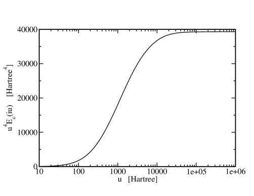
Figure 1: (Color online) $u^{4}E_{c}(iu)$ vs $u$ for He (maximum excitation energy $\delta\epsilon\approx 4000$ Hartree).

This behavior can be easily understood on the basis of Eq. (21): For frequencies beyond the maximum excitation energy $\delta\epsilon=\epsilon_{a\sigma}^{\rm max}-\epsilon_{i\sigma}$ included in the calculation (or provided by the basis set) $D_{ia\sigma}(u)$ and thus $S_{L}(u)$ decay as $u^{-2}$ which allows a perturbative evaluation of (33) in powers of $S_{L}(u)$, with the second order term dominating the resulting $E_{c}(iu)$.

On the other hand, for the more important range of large frequencies less than $\delta\epsilon$ a decay close to $u^{-3}$ is found, as shown in Figure 2.

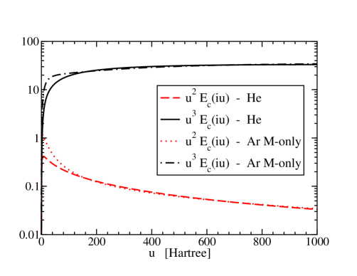
Figure 2: (Color online) $u^{2}E_{c}(iu)$ and $u^{3}E_{c}(iu)$ vs $u$ for moderately large $u$ for the case of He.

The same behavior is observed for each individual shell, as illustrated by the $E_{c}(iu)$ obtained by excitation of only the $M$-shell of neutral Ar, also included in Figure 2.

This power law decay suggests a transformation of the frequency interval $0\leq u<\infty$ to some finite interval via a power law transformation, as for instance

$$x=\frac{1}{1+(u/s)}\hskip 30.0pt0\leq x\leq 1\;,$$ (35)

giving more weight to large $u$ than an exponential transformation. The scale factor $s$ is intrinsically related to the minimum energy required for a virtual excitation, which is roughly given by the eigenvalue difference $\epsilon_{LUMO}-\langle\epsilon\rangle\approx|\langle\epsilon\rangle|$ for a shell with average eigenvalue $\langle\epsilon\rangle$. The most appropriate $s$ can only be determined empirically. For all atoms considered in detail the choice $s=2|\langle\epsilon\rangle|$ seemed to work reasonably well (see also below). The result of the transformation (35) is shown in Figure 3 for He, Ar¹⁶⁺ as well as the $M$-shell of neutral Ar.

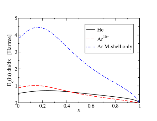
Figure 3: (Color online) Integrand $E_{c}(iu)du/dx$ of frequency integral after the transformation (35) vs $x$ for He, Ar¹⁶⁺ as well as the $M$-shell of neutral Ar.

One obtains a smooth function of $x$, with values remaining on the same order of magnitude for all $x$. This ensures a rapid convergence of the numerical integration over $x$ with the number of grid points.

However, the frequency integration in (5) suffers from the fact that each shell in an atom (or molecule) introduces a new energy scale for the virtual excitations. This is most easily verified by plotting $uE_{c}(iu)$ on a double logarithmic scale, as done in Figure 4 for He, Ne and Ar.

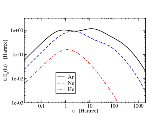
Figure 4: (Color online) $uE_{c}(iu)$ vs $u$ for Ne and Ar.

Figure 4 demonstrates that there are two relevant scales for Ne, three in the case of Ar. In fact, the plots confirm that the behavior of $E_{c}(iu)$ changes at roughly twice the average eigenvalues of the shells involved, with the position of the highest energy transition point being somewhat less pronounced ($\epsilon_{K}$(Ne)=$-30.8$, $\epsilon_{L}$(Ne)=$-1.1$; $\epsilon_{K}$(Ar)=$-114.4$, $\epsilon_{L}$(Ar)=$-9.4$, $\epsilon_{M}$(Ar)=$-0.7$ — all values in Hartree). It is therefore necessary to split the frequency integration from 0 to $\infty$ into intervals associated with these individual energy scales. Let us call the boundaries of the intervals $b_{i}$,

$$0=b_{0}<b_{1}<\ldots<b_{n}=\infty$$ (36)

with $n$ denoting the number of shells. The intervals are chosen such that the characteristic energy scale $s_{n}$ of shell $n$ is bracketed,

$$b_{i-1}<s_{i}<b_{i}\;.$$ (37)

In practice, $s_{i}=2|\langle\epsilon_{i}\rangle|$ and $b_{i}=4|\langle\epsilon_{i}\rangle|$ seemed to provide a reasonable partioning of the complete frequency range. Eq.(5) may then be decomposed as

$$\int_{0}^{\infty}E_{c}(iu)du=\sum_{i=1}^{n}\int_{b_{i-1}}^{b_{i}}E_{c}(iu)du\;.$$ (38)

In order to account for the piecewise decay of $E_{c}(iu)$ the transformation

$$x_{i} = \frac{[1+s_{i}/(b_{i}-b_{i-1})]}{[1+(u-b_{i-1})/s_{i}]}\,\frac{u-b_{i-1}}{s_{i}}$$ (39)

$$\frac{du}{dx_{i}} = s_{i}\,\frac{[1+s_{i}/(b_{i}-b_{i-1})]}{[1+s_{i}/(b_{i}-b_{i-1})-x_{i}]^{2}}$$ (40)

$(i=1,\ldots n)$ is most suitable. Eq.(38) can then be written as

$$\int_{0}^{\infty}E_{c}(iu)du = \sum_{i=1}^{n}\int_{-1}^{1}dx_{i}\frac{du}{dx_{i}}E_{c}(iu(x_{i}))\;.$$ (41)

The success of this frequency partioning plus power law transformation scheme is demonstrated in Figure 5, in which the final integrands $du/dx_{i}\,E_{c}(iu(x_{i}))$ are plotted for neutral Ar.

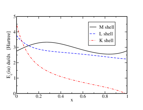
Figure 5: (Color online) Integrand $E_{c}(iu(x))du/dx$ of partioned frequency integral (41) resulting from the transformation (39) for neutral Ar.

In all three energy regimes a rather smooth integrand is obtained, which allows the application of Gauss-Legendre quadrature to each interval. As a result, the error obtained for a given total number of grid points $N_{u}$ used for the Gauss-Legendre quadrature is rather small already for very low $N_{u}$, as illustrated in Figure 6.

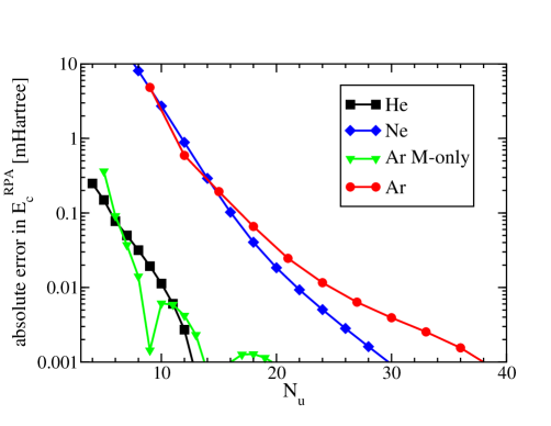
Figure 6: (Color online) Absolute error resulting from Eqs.(41) and (39) as a function the total number of grid points $N_{u}$ used for the Gauss-Legendre quadrature (note: $N_{u}$ is the sum of the number of grid points used in the individual intervals).

The most critical interval in Eq.(41) is the highest energy range, covering in particular excitations of the $1s$-state. For that reason the error is even lower if only excitations of the valence shell are included (i.e.  in the FC approximation), as is obvious from the error found for He or the $M$-shell of neutral Ar.

IV Results

IV.1 Sensitivity to form of KS orbitals

Table 4: Absolute RPA total energies (in Hartree) resulting from insertion of different KS orbitals. The last row lists the self-consistent RPA total energies given in Ref.Hellgren and von Barth, 2007.

KS orbitals	He	Be	Ne	Mg	Ar	N	Na
LDA	2.945	14.751	129.140	200.293	527.905	54.735	162.475
BLYP	2.944	14.752	129.142	200.296	527.910	54.737	162.478
EXX-only	2.945	14.752	129.143	200.298	527.913	54.738	162.480
RPA	2.945	14.754	129.143	200.296	527.908	—	—

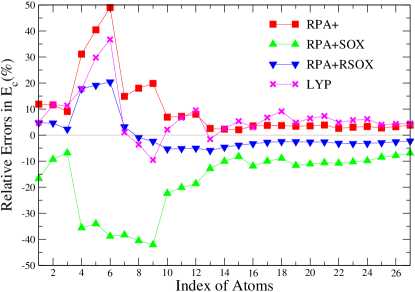
Figure 7: (Color online) Relative errors resulting from different approximate correlation energies, obtained from the data in Table 5.

Standard KS-DFT calculations are based on the self-consistent solution of the KS equations, which requires the evaluation of the XC potential $v_{\mathrm{xc}}(\mathbf{r})=\delta E_{\mathrm{xc}}[n]/\delta n(\mathbf{r})$. In the case of LDA and GGA functionals the calculation of $v_{\mathrm{xc}}(\mathbf{r})$ is straightforward. On the other hand, a self-consistent implementation represents a much more serious problem for RPA-type functionals. First of all, in the case of orbital-dependent functionals $v_{\mathrm{xc}}$ has to be determined via the OPM, i.e.  by solution of an integral equation.Talman and Shadwick (1976) The solution of the OPM integral equation is well-established for the exact exchange and managable, though rather intricate, for the second order correlation functional $E_{c}^{(2)}$.Grabowski et al. (2002); Yang and Wu (2002); Mori-Sanchez et al. (2005); Jiang and Engel (2005) Its implementation for RPA-type functionals, however, is much more challenging, so that a full solution has only been reported very recently.Hellgren and von Barth (2007) On the other hand, a self-consistent implementation is only then advantageous if the resulting correlation potential leads to an improved total KS potential. It has been demonstrated that this is not the case for some standard GGAs Umrigar and Gonze (1994) and for $E_{c}^{(2)}$, Jiang and Engel (2005, 2006) which by far overestimates correlation effects. The situation is not yet completely clear in the case of the RPA. The first RPA potentials available Hellgren and von Barth (2007) seem to improve over $v_{c}^{(2)}=\delta E_{c}^{(2)}/\delta n(\mathbf{r})$ in the asymptotic regime, but otherwise often follow $v_{c}^{(2)}$.

Independently of this more fundamental aspect, one might ask whether a self-consistent implementation is really necessary to obtain accurate RPA correlation and thus ground state energies. Clearly, a purely perturbative treatment of RPA-type functionals on the basis of a self-consistent calculation with the exact exchange would allow their application to much more complex systems, for which the solution of the corresponding OPM integral equation is beyond current computer resources. In fact, experience with conventional density functionals suggests that, at least for atomic systems, the RPA correlation energy is not sensitive to the detailed structure of $v_{\mathrm{xc}}(\mathbf{r})$.

In order to verify this expectation, the RPA ground state energy (i.e. the sum of the KS kinetic energy, the Hartree term, the exact exchange and $E_{\mathrm{c}}^{\mathrm{RPA}}$) has been calculated by insertion of KS orbitals resulting from different XC functionals: Orbitals obtained from self-consistent calculations with only the exact exchange (EXX-only), but neglecting $v_{\mathrm{c}}$ completely, are compared with self-consistent LDA and GGA orbitals. The results for a number of atoms are collected in Table 4, which also includes recent self-consistent RPA energies,Hellgren and von Barth (2007) whenever available. Table 4 confirms the expectation: Even though the KS potentials obtained by EXX-only calculations differ substantially from their LDA and GGA counterparts, the differences between the resulting RPA energies are quite small. The same is true for the deviations between the perturbative RPA energies on EXX-only basis and the self-consistent RPA results. This result is expected to hold quite generally, as long as one does not examine a quantity which is particularly sensitive to the correlation potential (as, for instance, the quantum defect of high Rydberg states van Faassen and Burke (2006)). In fact, Table 4 indicates that even a perturbative treatment of both the exact exchange and the RPA may be legitimate for very complex systems, in which even self-consistent calculations with the exact exchange are too expensive. In the following sections, self-consistent EXX-only orbitals are always used for the evaluation of the RPA correlation energy.

IV.2 RPA correlation energies of spherical atoms

In this work, we focus on atoms with closed or half-filled shells, for which the ground state KS potentials for the two spin-channels are both spherically symmetric.

Table 5: Absolute correlation energies (in Hartree) of closed sub-shell atoms calculated from the RPA and RPA+ functionals by insertion of the exact EXX-only KS orbitals in comparison with exact data. Chakravorty et al. (1993) The last row provides the mean absolute error (MAE) with respect to the exact energies.

atom	exact	RPA	RPA+	RPA+SOX	RPA+RSOX	LYP
He	0.042	0.083	0.047	0.035	0.044	0.044
Li+	0.043	0.087	0.048	0.039	0.045	0.048
Be2+	0.044	0.088	0.048	0.041	0.045	0.049
Li	0.045	0.112	0.059	0.029	0.053	0.053
Be+	0.047	0.122	0.066	0.031	0.056	0.061
B2+	0.049	0.131	0.073	0.030	0.059	0.067
Be	0.094	0.179	0.108	0.058	0.097	0.095
B+	0.111	0.205	0.131	0.066	0.110	0.107
C2+	0.126	0.228	0.151	0.073	0.123	0.114
N	0.188	0.335	0.201	0.146	0.178	0.192
O+	0.194	0.345	0.208	0.155	0.184	0.207
F2+	0.199	0.355	0.215	0.162	0.189	0.218
Ne	0.390	0.597	0.400	0.340	0.367	0.384
Na+	0.389	0.599	0.398	0.350	0.371	0.399
Mg2+	0.390	0.601	0.398	0.358	0.375	0.411
Na	0.396	0.626	0.410	0.349	0.383	0.408
Mg+	0.400	0.634	0.415	0.360	0.389	0.427
Al2+	0.405	0.642	0.420	0.369	0.395	0.442
Mg	0.438	0.687	0.453	0.387	0.427	0.459
Al+	0.452	0.706	0.468	0.402	0.440	0.481
Si2+	0.463	0.722	0.481	0.414	0.451	0.497
P	0.540	0.850	0.554	0.482	0.523	0.566
S+	0.556	0.873	0.573	0.499	0.538	0.588
Cl2+	0.570	0.893	0.589	0.514	0.552	0.605
Ar	0.722	1.101	0.742	0.661	0.701	0.751
K+	0.739	1.126	0.763	0.681	0.720	0.771
Ca2+	0.754	1.150	0.783	0.702	0.737	0.788
MAE		0.196	0.015	0.039	0.011	0.018

Table 5 lists the correlation energies obtained from all four RPA-based functionals for a series of atoms. To see trends more clearly, the relative errors resulting from the various functionals with respect to the exact correlation energies Chakravorty et al. (1993) are plotted in Figure 7. Not surprisingly, the pure RPA always overestimates the true correlation energy. Adding the short-range correction within the LDA (RPA+) improves the results remarkably, reducing the mean absolute error by more than an order of magnitude. As expected, the unscreened SOX contribution by far overcorrects the error of the RPA. On the other hand, the inclusion of EN-corrections into the SOX term (RSOX) reduces this overcorrection significantly. In general, both the RPA+ and the RPA+RSOX produce more accurate correlation energies than the LYP-GGA, at least for the set of atoms considered in this work. Moreover, for light atoms one observes a tendency of the RPA+RSOX to be superior to the RPA+.

IV.3 Ionization potentials

Even more important than the accuracy of total (correlation) energies is the accuracy of energy differences. In the case of atoms the ionization potential (IP) serves as the prototype energy difference for assessing the quality of any approximation. Much more than the total atomic $E_{c}$, the IP probes the description of the correlation of the valence states. We have therefore calculated the IPs resulting from the four RPA-based correlation functionals for a number of atoms. In order to avoid any uncertainty associated with spherical averaging, the comparison is restricted to atoms for which both the KS potential of the neutral ground state and that corresponding to the ionic state are spherical.

Table 6: First ionization potentials (in Hartree) of spherical atoms calculated from total energy differences (IP$=E_{\rm tot}(N-1))-E_{\rm tot}(N)$), using different XC functionals. The last row provides the mean absolute error (MAE) with respect to the exact results.Chakravorty et al. (1993) Self-consistent EXX-only KS orbitals are used as input orbitals.

atom	exact	EXX	RPA	RPA+	RPA+SOX	RPA+RSOX	BLYP
Li	0.198	0.195	0.220	0.205	0.185	0.203	0.201
Be+	0.669	0.666	0.700	0.683	0.656	0.677	0.681
Be	0.343	0.295	0.352	0.338	0.323	0.336	0.329
B+	0.924	0.861	0.935	0.919	0.897	0.912	0.904
Na	0.189	0.179	0.206	0.191	0.178	0.191	0.194
Mg+	0.552	0.540	0.573	0.557	0.543	0.555	0.566
Mg	0.281	0.242	0.294	0.279	0.268	0.279	0.279
Al+	0.691	0.643	0.706	0.691	0.677	0.688	0.691
MAE		0.028	0.017	0.005	0.015	0.005	0.009

The results are collected in Table 6. The most noteworthy features of these data are: (1) The pure RPA, though showing significant improvement over the EXX-only approximation, generally overestimates the true IPs; (2) Correspondingly, the RPA+SOX underestimates IPs (consistent with the unscreened nature of the pure SOX term); (3) Both the RPA+ and the RPA+RSOX significantly improve over the pure RPA results, and are even more accurate than BLYP, the “most accurate” standard GGA.

V Summary and Conclusions

In this work, we provide benchmark results for the RPA and three simple extensions, allowing for an unambiguous assessment of the functionals by comparison with exact data. Our results confirm earlier observations of the limited applicability of the pure RPA: The RPA substantially overestimates correlation energies, which then results in an overestimation of energy differences like ionization potentials. On the other hand, our results also demonstrate that already quite simple extensions of the RPA can be superior to standard GGAs: Adding either short-range corrections within the LDA (RPA+) or a suitably ’screened’ second order exchange contribution (RPA+RSOX) significantly improves both absolute energies and energy differences. This success is consistent with the expectation that the dominant source of error in the RPA functional is the missing short-range SOX contribution.

It seems worthwhile emphasizing that the first of these extensions, the RPA+, essentially comes at no cost: Compared to the computational demands of an RPA-calculation, the cost of the LDA for the non-RPA correlation is irrelevant. Moreover, a systematic improvement of the RPA+ by inclusion of gradient corrections for the non-RPA correlation contributions suggests itself. The RPA+RSOX involves an evaluation of the orbital-dependent SOX term, which is computationally almost as demanding as the calculation of the RPA energy itself, but still much less expensive than that of the fully screened SOX term.

In this work also several technical aspects of RPA-calculations have been studied systematically, of which two should be relevant beyond the regime of atoms considered here. The first of these aspects is the sensitivity of the RPA-expression to the orbitals and eigenvalues used for its evaluation. It turned out that the character of the KS spectrum inserted into the RPA has little impact on the resulting energy. Even if KS states obtained by LDA calculations are used the deviations from more accurate data remain small. In order to cover systems with more than one occupied shell, we have developed a partioning scheme for the frequency integration inherent in all RPA-type functionals, which, together with a suitable transformation of the integration variable, allows to perform the frequency integration with a minimum number of mesh points. Both these numerical techniques should be particularly helpful for applications to more complex systems.