Theory of radiation trapping by the accelerating solitons in optical fibers

Abstract

We present a theory describing trapping of the normally dispersive radiation by the Raman solitons in optical fibers. Frequency of the radiation component is continuously blue shifting, while the soliton is red shifting. Underlying physics of the trapping effect is in the existence of the inertial gravity-like force acting on light in the accelerating frame of reference. We present analytical calculations of the rate of the opposing frequency shifts of the soliton and trapped radiation and find it to be greater than the rate of the red shift of the bare Raman soliton. Our findings are essential for understanding of the continuous shift of the high frequency edge of the supercontinuum spectra generated in photonic crystal fibers towards higher frequencies.

I Introduction

Frequency conversion in optical fibers has been an active research field already for few decades Agrawal (2001). Most striking and extensively studied recent advance has been generation of extremely broad optical spectra (supercontinua) in optical fibers with small effective area, pumped by femto-second pulses with the carrier frequency close to the point of the zero group velocity dispersion (GVD) Ranka et al. (2000); Dudley et al. (2002). Applications of the supercontinuum include spectroscopy, metrology Holzwarth et al. (2000), telecommunication Smirnov et al. (2006) and medicine Hartl et al. (2001).

Amongst problems posed by the observation of supercontinuum one of the most puzzling has been understanding of the nonlinear processes leading to the generation of the high frequency wing of the supercontinuum continuously drifting towards even higher frequencies Husakou and Herrmann (2001); Washburn et al. (2002); Genty et al. (2002); Tartara et al. (2003); Austin et al. (2006). Several experimental and numerical observations explicitly demonstrated that the radiation at the blue wing of the supercontinuum often propagates in the form of nondispersive wave packets, localized on the femtosecond scale and continuously blue shifting Genty et al. (2004); Hori et al. (2004); Gorbach et al. (2006); Frosz et al. (2005). Note that GVD at the blue edge of the continuum is typically normal, therefore the dispersive spreading can not be compensated by the nonlinearity. Independently from the supercontinuum generation the effect of the localization of blue shifting pulses in the normal GVD range, coupled to the Raman solitons propagating in the anomalous GVD range, has been reported in the series of papers by Nishizawa and Goto Nishizawa and Goto (2002a, b, c) and more recently by Cheng and co-authors Cheng et al. (2005). It has been proposed in Refs. Nishizawa and Goto (2002a, b, c); Cheng et al. (2005) that the physical mechanism behind the above effects is the cross-phase modulation (XPM) Agrawal (2001); Manassah (1988).

However, it is well known that the XPM coupling between anomalously and normally dispersing components can lead to dispersion compensation and formation of the bright-dark soliton pairs only if one soliton component is a dark pulse and the other one is bright, see, e.g., Trillo et al. (1988); Kivshar (1992); Buryak et al. (1996). Thus the XPM can not be the sole reason for formation of the bright-bright localized states across the zero GVD wavelength Genty et al. (2004); Hori et al. (2004); Gorbach et al. (2006); Frosz et al. (2005); Nishizawa and Goto (2002a, b, c). Also, the red shift of the anomalously dispersing component is readily explained by the intrapulse Raman scattering Agrawal (2001); Gordon (1986), while the blue shift of the normally dispersing bright pulse coupled to it requires to be understood.

Reference Gorbach et al. (2006) has explained formation of the blue edge of supercontinua in fibers using the theory of four-wave mixing between the solitons and dispersive waves Skryabin and Yulin (2005); Efimov et al. (2005). It has been demonstrated that for typical fiber dispersions the interaction between the soliton and the blue radiation happens recurrently, so that every scattering event leads to the further blue shift of the signal pulse Gorbach et al. (2006). Though this theory describes well first stages of the blue edge formation it fails to explain why the femtosecond pulses emerging there remain free of dispersive spreading. The latter is naturally expected because of the strong normal GVD and would lead to a fast degradation of any nonlinear interaction between the soliton and the blue radiation, which in practice continues over long distances. In our recent work Gorbach and Skryabin (2007) we have explained the physical mechanisms behind existence of the non-dispersive and continuously blue shifting localized states of light on the high frequency edge of the supercontinuum spectra. The light is trapped by the refractive index changes induced, on one side (front of the pulse), by the red shifting Raman solitons via the nonlinear cross coupling and, on the other side (trailing tail), by the inertial force originating from the fact that the solitons move with acceleration. The nature of the latter effect is analogous to the gravity-like inertial force acting on an observer in a rocket moving with a constant acceleration.

The aim of this work is not only to provide mathematical details for the mostly qualitative description presented in Gorbach and Skryabin (2007), but also to extend the theory into the regime of sufficiently strong intensities of the blue radiation. In this regime the trapped blue component of the two frequency bound-state starts to influence the soliton dynamics on the red edge, which makes noticeable quantitative impact on the propagation dynamics of the bound state.

II The model

The subject of this work is the explanation of the existence and detailed study of the previously reported Genty et al. (2004); Hori et al. (2004); Gorbach et al. (2006); Frosz et al. (2005); Nishizawa and Goto (2002a, b, c); Cheng et al. (2005) two-frequency bright-bright soliton-like states in optical fibers, with frequency of one component being in the anomalous and frequency of the other being in the normal GVD range. Thus the dispersion we need to use should include the sign change of the GVD. The simplest example of the dispersion operator having this property is

$$\partial_{z}E-{1\over 6}\epsilon\partial_{t}^{3}E=0\;.$$ (1)

Assuming $E=e^{ikz-i\delta t}$, we find that the GVD is $\partial_{\delta}^{2}k=\epsilon\delta$. Thus $\delta$ measures the spectral deviation from the zero GVD point at $\delta=0$. The third-order dispersion coefficient $\epsilon$ is positive for the telecom fibers and in the proximity of the $800$nm for the typical photonic crystal fiber (PCF) designs used for generation of supercontinuum with femtosecond pulses Ranka et al. (2000); Dudley et al. (2002). $\epsilon$ can also be negative in the proximity of $1500$nm in PCFs and tapered fibers with sufficiently small cores Skryabin et al. (2003). It is important to note that the group index parameter $\partial_{\delta}k=\epsilon\delta^{2}/2$ is symmetric with respect to $\delta\to-\delta$ and therefore the group velocity is matched across the zero GVD point. The matching, or near matching, of the group velocities is important for the existence of the two-frequency bound states, because the pulses should not spatially separate before the bound state is established. In the PCFs the third order dispersion $\partial^{3}_{\delta}k$ usually changes its value and sign as frequency varies, as can be seen from the change of slope of the GVD curve in Fig. 1(b). This eventually destroys the matching of the group velocities across the zero GVD point, see Fig. 1(a). However, the fact that the matching is still achieved over the wide bandwidth is the most important for the effect of radiation trapping and for the formation of the blue wing of a supercontinuum.

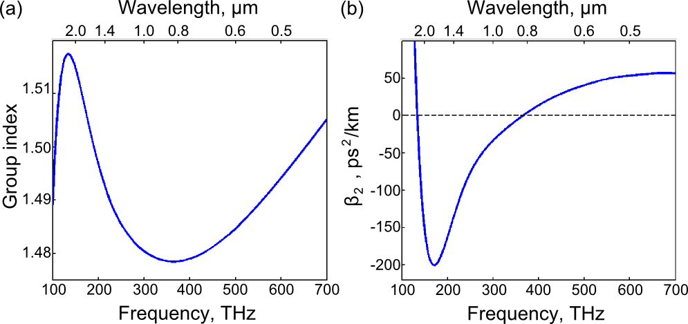
Figure 1: (Color online) Frequency dependence of the group velocity normalized to speed of light in vacuum (group index) (a) and of the GVD (b) in the photonic crystal fiber as in Ref. Gorbach et al. (2006). Fiber dispersion like this is typical for numerous supercontinuum experiments.

Taking into account the instantaneous Kerr nonlinearity and the non-instantaneous Raman response, the light propagation in a fiber is modeled by the dimensionless generalized nonlinear Schrödinger (NLS) equation Agrawal (2001)

$$\partial_{z}E=i\hat{k}(i\partial_{t})E+i(1-\theta)E|E|^{2}$$

$$+E\int_{-\infty}^{+\infty}{R(t^{\prime})|E(t-t^{\prime},z)|^{2}}dt^{\prime}.$$ (2)

The dispersion operator in Eq. (2) is

$$\hat{k}(i\partial_{t})\equiv\sum_{m=3}^{M}{L\beta^{(m)}\over\tau^{m}m!}[i\partial_{t}]^{m},$$ (3)

where the coefficients $\beta^{(m)}$ are selected to fit the dispersion profile of the fibers. The total electric field is given by $Ee^{ik_{r}z-i\omega_{r}t}+c.c.$, where the reference frequency $\omega_{r}$ is chosen to coincide with the zero GVD frequency, that is why the sum in Eq. (3) starts from $m=3$. $R(t)$ is the standard Raman response function of silica:

$$R(t)=\theta{\tau_{1}^{2}+\tau_{2}^{2}\over\tau_{1}\tau_{2}^{2}}\Theta(t)e^{-t/\tau_{2}}\sin{t\over\tau_{1}}\;.$$ (4)

Here $\Theta(t)$ is the Heaviside function and parameter $\theta=0.18$ weights the Raman nonlinearity relative to the Kerr one. Characteristic times of the delayed Raman response are $\tau_{1}=12.2fs/\tau$ and $\tau_{2}=32fs/\tau$ Agrawal (2001). $t$ is the dimensionless time in the reference frame moving with the light group velocity at $\omega_{0}$ and measured in the units of $\tau$. $z$ is the distance along the fiber measured in the units of $L$, where $L$ is any convenient characteristic length. Field amplitude $E$ is scaled to $1/\sqrt{\gamma L}$, where $\gamma$ is the nonlinear parameter of the fiber Agrawal (2001). To get feel for the real values of the parameters we choose $\gamma=0.02$(Wm)^-1 and $L=8$m, which gives $1/(\gamma L)=6.25$W. Choosing $\tau=200$fs and $\beta^{(3)}=0.12ps^{3}/km$ [corresponding to the dispersion slope at the zero GVD point close to $800$nm in Fig. 1(b)] we have $\epsilon=L\beta^{(3)}/\tau^{3}=0.12$.

III Numerical experiments illustrating radiation trapping by accelerating solitons

We proceed describing two sets of numerical experiments. First, is when supercontinuum evolves from a single pump pulse. Second, is when the two-frequency bound state is excited directly by the two pulses. In the first set we used the realistic fiber dispersion, see Fig. 1. However, to explain the effect of radiation trapping by solitons across the zero GVD point it is sufficient to consider the simple cubic dispersion as in Eq. (1), which simplifies comparison of analytical and numerical results and is used throughout the rest of the paper.

Figs. 2 illustrate supercontinuum generation with a single pump in the fiber as in Fig. 1. The pump frequency was chosen either in the range of anomalous GVD, Figs. 2(a),(b), or in the range of normal GVD Figs. 2(c),(d). In both cases one can see that, after the initial stages of the supercontinuum development (see e.g. Gorbach et al. (2006), for detailed description), the blue tip of the spectrum starts its continuous drift towards higher frequencies, see $z>0.2m$ in Fig. 2(a) and $z>1m$ in Fig. 2(c). This spectral shift appears to be correlated with the soliton self-frequency shift at the opposite (infrared) edge of the spectrum. Spectrograms showing the signals simultaneously in the frequency and time domains, see Figs. 2(b) and (d), unambiguously demonstrate that the high frequency tip of the continuum is localized in the time domain on the same femtosecond scale as the soliton at the infrared edge. One can also see, that not only the soliton at the very edge of the spectrum, but all the red shifting solitons have associated localized pulses on the high frequency side of the spectrum in the normal GVD range.

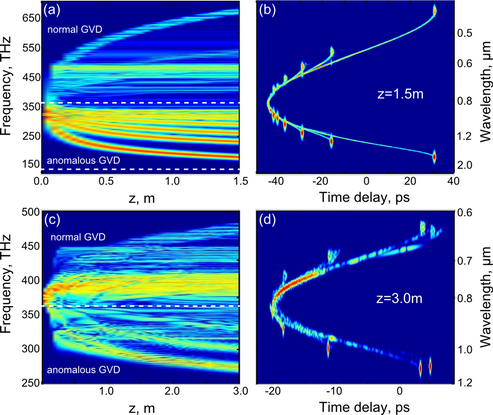
Figure 2: (Color online) Left panel: spectral evolution along the fiber length for the dispersion profile as in Fig. 1. Pump pulse parameters: (a) wavelength $900$nm is in the anomalous GVD range, (c) $800$nm is in the normal GVD range. In both cases peak power is $6$kW, duration $200$fs; The radiation at the short wavelength edge of the continuum starts its continuous drift towards shorter frequencies at $z>0.2m$ for (a) and $z>1m$ for (c). Right panel: spectrograms showing simultaneous frequency and time domain images of the supercontinua in (a) and (c) for $z=1.5m$ and $z=3m$, respectively. The function plotted has been calculated using the XFROG integral $I(t,\omega)=\int_{-\infty}^{\infty}$ $dt^{\prime}E_{ref}(t^{\prime}-t)E(t^{\prime})e^{-i\omega t^{\prime}}$. Here $E_{ref}$ is the $2$ps gaussian pulse. See Ref. Trebino (2000) on more details about the XFROG (cross-correlation frequency resolved optical gating).

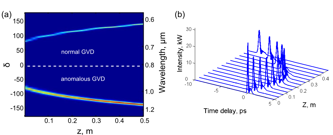
Figure 3: (Color online) Spectral (a) and time-domain (b) evolution along the fiber pumped with two pulses obtained from the numerical modeling of Eq. (2) with $\beta^{(m>3)}=0$ and $\epsilon=+0.12$. Initial conditions are $E(z=0,t)=\sqrt{2q_{1}}\textrm{sech}(t/\tau_{1})\exp(-i\delta_{1}t)+\sqrt{2q_{2}}\textrm{sech}((t-T_{0})/\tau_{2})\exp(-i\delta_{2}t)$. with $q_{1}=2000$ (peak power $\sim 24kW$), $q_{2}=250$ (peak power $\sim 3kW$), $\tau_{1}=\sqrt{-D^{\prime\prime}_{s}/2q_{1}}=0.2$ ($\sim 40fs$), $\tau_{2}=\sqrt{-D^{\prime\prime}_{s}/2q_{2}}\approx 0.57$ ($\sim 115fs$), $T_{0}=0.25$ ($\sim 50fs$) and $\delta_{1}=-80$ ($\sim 964nm$), $\delta_{2}=80$ ($\sim 684nm$). Results in (b) are presented in the accelerating frame of reference: $t^{\prime}=t-g_{0}z^{2}/2$, with $g_{0}$ defined by Eq. (15).

To isolate the effect of formation of the two-frequency bound-states across the zero GVD point we perform simulations using the two pulse excitation. From now on we will focus on the simple case of cubic dispersion as in Eq. (1). We start from the case $\epsilon>0$, see Fig. 3. The first of the pump pulses is spectrally located in the anomalous GVD regime and forms a red shifting Raman soliton. The second pulse is delayed with respect to the first one and has spectrum in the range of normal GVD. In the course of the propagation the latter pulse appears to be trapped on the trailing tail of the soliton, while its frequency is continuously increasing, see Fig. 3. Note that the Raman effect pulls the soliton toward smaller frequencies and away from the zero GVD point, therefore the GVD felt by the soliton is continuously increasing. This leads to the noticeable temporal broadening of the soliton and to the drop in its amplitude, which also affects the shape of the trapped radiation, see Fig. 3(b). Clearly the group velocities of the two components within the bound state are the same, which suggests that the frequencies are changing along the dispersion curve in such a way that the group velocity matching is preserved.

In the case of the negative third-order dispersion ($\epsilon<0$) the effect of the radiation trapping is also clearly observed, see Fig. 4. The difference here is that the normally and anomalously dispersing components of the two-frequency bound-state are now spectrally converging towards the zero GVD point, see Fig. 4(a). However, the direction of the spectral evolution of each of the components is the same as for $\epsilon>0$. Namely the Raman effect pulls the soliton component in the anomalous GVD range towards smaller frequencies, while the pulse in the normal GVD range shifts towards higher frequencies. The GVD felt by the soliton is reducing in this case, therefore the soliton is adiabatically compressed, see Figs. 4(b), (f). When the soliton is pulled sufficiently close to the zero GVD point, so that the significant part of its own spectrum is in the normal GVD regime, it starts to emit Cherenkov radiation Wai et al. (1990); Karpman (1993); Akhmediev and Karlsson (1995), see Figs. 4(a), (e). This radiation creates spectral recoil effect, which counterbalances the Raman self-frequency shift and stabilizes the soliton frequency Skryabin et al. (2003); Biancalana et al. (2004). As the soliton looses its energy through radiation, it broadens and so does the trapped wavepacket. Still, both spectral components of the bright-bright quasi-soliton pair remain fairly well localized over propagation distances much larger than the GVD length. Spectrograms showing the effect of the radiation trapping in this case are shown in Figs. 4 (c), (d). Note, that the stabilization of the frequency of the pure soliton, i.e. without the trapped radiation, happens at longer propagation distances, cf. Figs. 4(a) and (e). This suggests that the trapping effect boosts the rate of the soliton self frequency shift. We will discuss this more in details in Sec. VI.

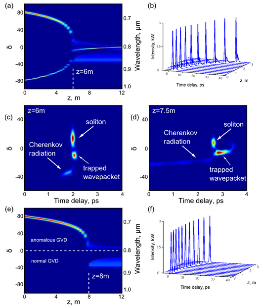
Figure 4: (Color online) Pulse propagation in the case of negative third-order dispersion, $\epsilon=-0.12$. (a) and (b): two pulses pump similar to that in Fig. 3. Parameters of the pulses are: $q_{1}=200$ (peak power $=\sim 2.4kW$), $q_{2}=25$ (peak power $\sim 0.3kW$), $\tau_{1}=\sqrt{-D^{\prime\prime}_{s}/2q_{1}}\approx 0.63$ ($\sim 130fs$), $\tau_{2}=\sqrt{-D^{\prime\prime}_{s}/2q_{2}}\approx 1.8$ ($\sim 360fs$), $T_{0}=1.5$ ($\sim 300fs$) and $\delta_{1}=80$, $\delta_{2}=-80$. (c) and (d): XFROG spectrograms for the case of two-pulse pump, calculated at different propagation distances. (e) and (f): soliton propagation with $q=200$ (peak power $\sim 2.4kW$). All time domain results are presented in the accelerating frame of reference: $t^{\prime}=t-g_{0}z^{2}/2$, with $g_{0}$ defined by Eq. (15).

IV Coupled NLS equations in the accelerated frame of reference

In order to explain the above numerical observations of the two-frequency bound states across the zero GVD point, we reduce Eq. (2) to the coupled NLS equations for the two pulses on the opposite sides of the zero GVD frequency. We assume

$$E=A_{1}\exp[ik_{1}z-i\delta_{1}t]+A_{2}\exp[ik_{2}z-i\delta_{2}t],$$ (5)

where $A_{1,2}$ are the amplitudes of the two pulses, $\delta_{1,2}$ are their frequencies and $k_{1,2}=k(\delta_{1,2})$ are the wavenumbers: $k(\delta)=e^{i\delta t}\hat{k}(i\partial_{t})e^{-i\delta t}$. We also assume that $\delta_{1,2}$ are selected in such a way that $k_{1}^{\prime}=k^{\prime}_{2}$ ($k^{\prime}=\partial_{\delta}k$) and therefore the group velocities of the two pulses are equal. Substituting Eq. (5) into Eq. (2), expanding $|E(t-t^{\prime})|^{2}$ in Eq. (2) up to the first order Taylor term and neglecting all the fast oscillating exponential terms with frequencies $\delta_{1,2}$ and their harmonics we obtain a pair of the coupled NLS equations:

$$i\partial_{z}A_{1}+d_{1}\partial^{2}_{x}A_{1} = -\left[|A_{1}|^{2}+2|A_{2}|^{2}\right]A_{1}+$$ (6)

$$TA_{1}\partial_{x}\left[|A_{1}|^{2}+|A_{2}|^{2}\right]\;,$$

$$i\partial_{z}A_{2}+d_{2}\partial^{2}_{x}A_{2} = -\left[|A_{2}|^{2}+2|A_{1}|^{2}\right]A_{2}+$$ (7)

$$TA_{2}\partial_{x}\left[|A_{1}|^{2}+|A_{2}|^{2}\right]\;,$$

where $x=(t-zk_{1}^{\prime})/\sqrt{|k_{1}^{\prime\prime}|}$, $T=|k^{\prime\prime}_{1}|^{-1/2}\tau_{d}$ is the effective Raman time, $\tau_{d}=\int tR(t)dt\approx 0.0073$, $d_{1}=1/2$ (anomalous GVD), and $d_{2}=-|k^{\prime\prime}_{2}|/|2k^{\prime\prime}_{1}|<0$ (normal GVD). The most important restriction of Eqs. (6), (7) relative to Eq. (2) is that the former do not include frequency dependence of the GVD, see Fig. 6. However, this is not critical for understanding of the trapping mechanisms.

If $A_{2}=0$ then Eq. (6) has an approximate solution in the form of the NLS soliton moving with constant acceleration $g$ Agrawal (2001). So that its center in the $(x,z)$-plane follows the parabolic trajectory $x=gz^{2}/2$ and its frequency is continuously red shifting with the rate $g/(2d_{1})$. For the single NLS equation it has been demonstrated that there exist a transformation into the accelerating frame of reference, which retains the structure of the NLS equation apart from adding a linear in $x$ potential Chen and Liu (1976). $g$ is a free parameter of this symmetry transformation, which value is fixed by assuming that the corrections to the soliton induced by the linear potential are balanced by the corrections due to the Raman term, see below.

Here we apply the analogous symmetry transformation to the coupled equations

$$A_{1}=\psi\left(z,\xi\right)\exp\left[i\frac{\xi\dot{x}_{0}}{2d_{1}}+if_{1}(z)+iqz\right]\;,$$ (8)

$$A_{2}=\phi\left(z,\xi\right)\exp\left[i\frac{\xi\dot{x}_{0}}{2d_{2}}+if_{2}(z)+i\lambda z\right]\;,$$ (9)

where

$$\xi=x-x_{0}(z),~{}x_{0}=gz^{2}/2,~{}f_{1,2}(z)=-\frac{1}{4d_{1,2}}\int\dot{x}_{0}^{2}dz.$$ (10)

Parameters $q$ and $\lambda$ are the shifts of the propagation constants of the two components.

The resulting equations for $\psi$ and $\phi$ are

$$i\partial_{z}\psi+d_{1}\partial^{2}_{\xi}\psi = q\psi-\left[|\psi|^{2}+2|\phi|^{2}\right]\psi+$$ (11)

$$T\psi\partial_{\xi}\left[|\psi|^{2}+|\phi|^{2}\right]+\frac{g\xi}{2d_{1}}\psi\;,$$

$$i\partial_{z}\phi+d_{2}\partial^{2}_{\xi}\phi = \lambda\phi-\left[|\phi|^{2}+2|\psi|^{2}\right]\phi+$$ (12)

$$T\phi\partial_{\xi}\left[|\psi|^{2}+|\phi|^{2}\right]+\frac{g\xi}{2d_{2}}\phi\;.$$

The prime difference of the coupled NLS equations (11), (12) with the text book ones Agrawal (2001) is the presence of the linear in $\xi$ potentials. The acceleration $g$ has been the free parameter upto now. Its selection will be discussed in the next two sections.

We should note here, that the natural next step in our analysis could be the setting up a boundary value problem for the $z$-independent version of Eqs. (11), (12). However, proper setting of the boundary conditions is a challenging problem due to presence of the linear potential. The main reason for this is that working out asymptotic behavior of solutions for $\xi\to-\infty$ requires a delicate analysis going beyond the scope of this work. Indeed, if one simply neglects the nonlinearity, then the tails of both components behave like Airy functions, which was assumed in the prior works on the similar problems Akhmediev et al. (1996); Aleshkevich et al. (2000); Facão and Parker (2003). However, the amplitude of the oscillatory tail ($\xi\to-\infty$) of the Airy function decays only as $|\xi|^{-1/4}$, which makes some linear terms in Eqs. (11), (12) to decay at the rates matching the decay rate of the nonlinear terms, suggesting that equating the solution tails to the Airy function is an approximation. This problem still waits for its proper analysis even in the case of the single soliton equation. For the above reasons we rely in what follows on perturbation theory complemented by the numerical calculations with zero boundary conditions for large $|\xi|$, which correctly describes the localized parts of the solutions, but gives only qualitative answers at the oscillatory tails. The effects we study below are, however, dependent most strongly on the localized part of the solutions, and therefore our approximation is adequate in the given context.

V Linear theory of the radiation trapping

We proceed, by considering the limit when the normally dispersive component $\phi$ is much weaker than the soliton component $\psi$. In this limit we can assume that the field $\psi$ is not affected by $\phi$ and neglect all the terms nonlinear in $\phi$. Then Eq. (11) for $\psi$ can be solved perturbatively. We assume $\psi=\psi_{0}(\xi)+\psi_{1}(\xi)+\dots$, where

$$\psi_{0}={\sqrt{2q}}{\textrm{sech}(\sqrt{q/d_{1}}\xi)}$$ (13)

solves $d_{1}\partial_{\xi}^{2}\psi_{0}=q\psi_{0}-\psi_{0}^{3}$ and $\psi_{1}$ accounts for corrections due to Raman effect and the linear potential:

$$d_{1}\partial_{\xi}^{2}\psi_{1}-q\psi_{1}+3\psi_{0}^{2}\psi_{1}=T\psi_{0}\partial_{\xi}\psi_{0}^{2}+{g\xi\over 2d_{1}}\psi_{0}.$$ (14)

The operator $d_{1}\partial_{\xi}^{2}-q+3\psi_{0}^{2}$ is self-adjoint and singular. Its null space is spanned by the single eigenfunction $\partial_{\xi}\psi_{0}$. Projecting the right-hand side of Eq. (14) on the latter we find

$$g=g_{0}\equiv{32Tq^{2}\over 15}\;.$$ (15)

Thus the linear potential indeed compensates for the Raman shift, at least in the first order, providing $g=g_{0}$. Note, that this approach neglects the non-exponential decay of the soliton tail at $\xi\to-\infty$, see discussion at the end of the previous section, and it is equivalent to the traditional considerations Gordon (1986); Chen and Liu (1976), where the oscillatory tail has been ignored.

The $z$-independent equation for $\phi$ is simply a linear eigenvalue problem in our approximation

$$-|d_{2}|\partial^{2}_{\xi}\phi+V(\xi)\phi=\lambda\phi,$$ (16)

where potential $V(\xi)$ consists of the localized soliton part and of the linear potential induced by the acceleration with already determined value:

$$V(\xi)=2\psi_{0}^{2}-T\partial_{\xi}\psi_{0}^{2}+\frac{g_{0}\xi}{2|d_{2}|}.$$ (17)

The superposition of the exponentially decaying soliton tail and of the linear potential creates a local minimum of $V$ on the trailing tail of the soliton, see Fig. 5(a), giving rise to the effect of light localization in the normal GVD regime. The soliton itself serves as a potential barrier for the normally dispersive waves on one side of the well and the linear potential, obtained as a result of the transformation to the accelerated frame of reference, serves as a barrier on the other side. Thus the accelerating potential creates an inertial force acting on photons. It is analogous to the gravity-like force acting on massive bodies in a closed container moving with a constant acceleration. The soliton created potential wall is not infinite, however. Therefore the light is expected to tunnel through it. Hence, only quasi-bound states embedded inside the continuum are possible as solutions of Eq. (16).

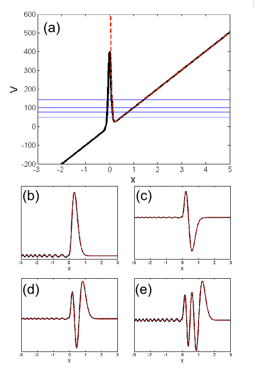
Figure 5: (Color online) (a) Full (dashed) line shows the potential $V$ ($V_{b}$) for the soliton with $q=100$ and $T=0.0024$. (b-e) show selected quasi-bound eigenstates of the potential $V$, cf. horizontal levels in (a). Dashed lines show the corresponding modes of the potential $V_{b}$.

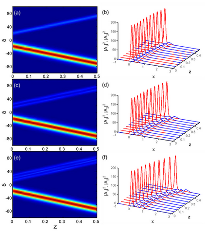
Figure 6: (Color online) Numerical propagation of the first three bound states within coupled equations (6), (7). Initial conditions are: soliton for $A_{1}$ with $q=100$ and linear eigenstate of $V$ for $A_{2}$. Left column: spectrum of the total field $E$, Eq. (5), with $\delta_{2}=-\delta_{1}=20$. Right column: temporal profiles of $|A_{1}|^{2}$ (dashed lines) and $|A_{2}|^{2}$ (solid lines). Time domain results are presented in the accelerating frame of reference: $t^{\prime}=t-g_{0}z^{2}/2$, with $g_{0}$ defined by Eq. (15).

In order to locate these states we first replace the soliton part of $V$ by its asymptotic and find that

$$V\approx V_{b}\equiv A\exp(-B\xi)+C\xi,$$ (18)

$$A=16q,~{}B=2\sqrt{\frac{q}{d_{1}}},~{}C=\frac{g_{0}}{2|d_{2}|}.$$

Contribution to $A$ due to the Raman term ($\sim T$) is small as compared to $16q$ and is neglected. The potential $V_{b}$ goes to infinity on both sides and has the discrete set of true bound states with eigenvalues $\lambda_{n}^{(b)}$. Eq. (16) with $V$ replaced by $V_{b}$ has been solved numerically and some of its eigenstates are shown in Fig. 5 with dashed lines. Then we take the finite potential $V$ and for each $n$ find few eigenvalues and corresponding eigenstates in the spectral proximity of $\lambda_{n}^{(b)}$, applying the zero boundary conditions at both ends. The latter implies that we reliably calculate only the states with relatively small tail amplitude at $\xi\to-\infty$. Having attempting more precise calculations would go beyond our original level of precision anyway, because the oscillations of the soliton tail at $\xi\to-\infty$ have been disregarded in the first place. Some quasi-bound eigenstates of the true potential $V$ are shown in Fig. 5(b)-(e) with the full lines, and the corresponding eigenvalues are indicated in Fig. 5(a).

The terms $\exp\left[\xi\dot{x}_{0}/(2d_{1,2})\right]$ in Eqs. (8), (9) explicitly express the continuous frequency shifts of the two components with the rates $g/2d_{1,2}$. The anomalous GVD ($d_{1}>0$) corresponds to the expected red frequency shift Gordon (1986). However, the normal GVD ($d_{2}<0$) implies the blue frequency shift. The latter explains spectral dynamics of the trapped radiation. Note, that some analogy may exist here with the previously reported blue shift of the spectral holes associated with the dark fiber solitons existing in the normal GVD range tomlin .

Equations (8), (9) give, however, little physical insight into which elementary wave scattering mechanisms lead to these opposing frequency shifts. The physical process driving the red shift of the soliton component is the well known intrapulse Raman scattering Agrawal (2001); Gordon (1986). The blue shift of the radiation component is driven by the intrapulse four-wave mixing described in details in Gorbach et al. (2006). Briefly, it means that the scattering of the radiation pulse on the soliton generates the blue shifted pulse. The continuous frequency shift of the soliton and the phase matching conditions work out in such a way that the observable result of this process is the continuous blue shift of the radiation pulse carrier frequency. Trapping effect sustains this process over the long propagation distances and results in existence of the stationary soliton-radiation states.

In order to verify validity of our approximate eigenvalue analysis we have initialized Eqs. (6), (7) with the soliton for $A_{1}$ and the linear eigenstates of $V$ for $A_{2}$ and solved the equations numerically. Fig. 6 shows evolution of the first three quasi-bound eigenstates. The amplitude of the eigenstates has been kept small in order to ensure that we remain in the regime, when $|A_{2}|^{2}$ terms are negligible. One can see that, despite using the simplified boundary conditions, our solutions satisfy well the coupled NLS equations. This simulation also confirms that the propagation distances on which the tunneling induced losses lead to noticeable effects are much larger than the typical GVD length. So that for the fiber length of order meters the dispersive spreading of the high frequency radiation is suppressed and it propagates as a localized state of light. Note also, that the characteristic feature of each quasi-bound state, apart from the lowest one, is the presence of several spectral peaks. Such multi-peak spectral structures are typical for the blue wing of supercontinua seen in Figs. 2(a), (c).

Approximation $V\approx V_{b}$ is also useful because it allows us to carry out explicit variational calculations of the eigenvalues and eigenfunctions, and thus to have analytical estimates for the width of the trapped states. Let us consider the variational approximation for the ground state ($n=0$) only. As a trial function we choose

$$\tilde{\phi}_{0}=\exp\left[-(\xi-\gamma)^{2}/w^{2}\right]\;,$$ (19)

where $\gamma$ is the shift of the intensity maximum of the trapped state with respect to the soliton one and $w$ is the width of trapped state. One can suggest a better trial functions accounting for the asymmetry of the profile of the ground. However, our choice is the best suited for getting transparent analytical expressions for parameters $\gamma$ and $w$. The variational estimate $\tilde{\lambda}_{0}$ for the true value $\lambda_{0}\leq\tilde{\lambda}_{0}$ is

$$\tilde{\lambda}_{0}=\frac{\int d\xi\;\tilde{\phi}_{0}\left[-|d_{2}|\partial^{2}_{\xi}+V_{b}\right]\tilde{\phi}_{0}}{\int d\xi\;\tilde{\phi}_{0}^{2}}$$ (20)

Minimizing $\tilde{\lambda}_{0}$ with respect to $\gamma$ and $w^{2}$ we find

$$w^{2} = 2\sqrt{\frac{2|d_{2}|}{BC}}=\frac{|d_{2}|}{2q}\sqrt{\sqrt{\frac{d_{1}}{q}}\frac{15}{2T}},$$ (21)

$$\gamma = \frac{B}{4}\sqrt{\frac{2|d_{2}|}{BC}}-\frac{1}{B}\ln\left(\frac{C}{BA}\right),$$ (22)

$$\tilde{\lambda}_{0} = \sqrt{\frac{|d_{2}|BC}{2}}+\frac{C}{B}\left[1-\ln\left(\frac{C}{BA}.\right)\right]$$ (23)

Thus the narrow solitons (large $q$) and large Raman effect (large $T$) result, quite naturally, in stronger localization of the radiation. Figure 7(a) illustrates comparison between the numerically calculated linear mode $\phi_{0}$ of the potential $V(\xi)$ (17) and the variational approximation. The numerically calculated dependencies $\lambda_{0}(q)$ and $\lambda_{0}^{(b)}(q)$ for potentials $V$ and $V_{b}$, respectively, compare well with the variational result (23), see Fig. 7(b).

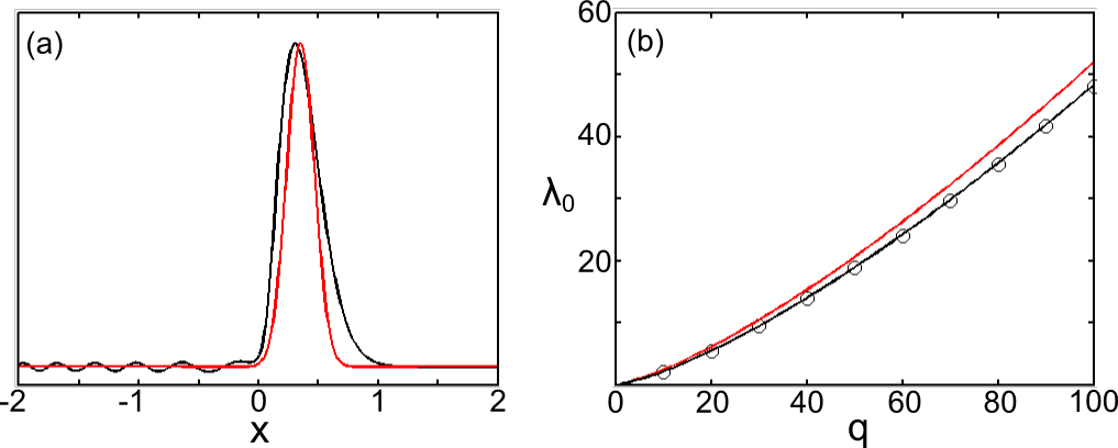
Figure 7: (Color online) (a) Lowest trapped linear mode of the potential $V$ (solid line) and its variational approximation (dashed line), given by Eq. (19) with $\gamma$ and $w^{2}$ defined through (22) and (21), respectively. Soliton parameter is $q=100$. (b) $\lambda_{0}^{(b)}(q)$, solid line, $\lambda_{0}(q)$, circles, and $\tilde{\lambda}_{0}(q)$, dashed line.

VI Nonlinear theory of the two-frequency quasi-solitons across the zero GVD point

The theory presented above explains the nature of the radiation trapping and is adequate in the regime when the radiation is weak. In this regime the family of the soliton-radiation bound states is continuously parameterized by $q$ only, i.e. by the amplitude of the soliton pulse. In particular, this is expressed in the fact that the acceleration parameter $g=g_{0}$ and the eigenvalue $\lambda$ are fixed for a given $q$. In the nonlinear regime one should expect that $\lambda$ will become a continuously varying parameter, as it happens for other types of localized solutions in incoherently coupled NLS equations Buryak et al. (1996). Thus the acceleration $g$ is expected to be continuously parameterized by both $q$ and $\lambda$, i.e. by the energies of the both fields $\phi$ and $\psi$. In order to demonstrate explicitly, that indeed there is a problem to be addressed here, we compare the propagation distance at which the spectral recoil from the Cherenkov radiation stabilizing the soliton frequency takes place with and without the blue detuned pulse seeded into the fiber. One can see, Figs. 4(a) and (e), that the sharp transition to the regime without the self-frequency shift happens at a shorter distance with the blue radiation present. This is because the spectral peak of the soliton reaches the critical distance from the zero GVD point sooner, which indicates that the rate of the self-frequency shift is faster for the soliton-radiation bound state than for the pure soliton, i.e. $g>g_{0}$. Thus nonlinear in $\phi$ corrections should be taken into account to explain this effect.

One obvious small parameter in our problem is the Raman time $T$, which enters both equations for $\phi$ and $\psi$. The linear in $\xi$ potential can be considered as a small perturbation only in the equation for $\psi$. However, it plays a crucial role in the localization of the $\phi$ component at $\xi\to\infty$ and therefore can not be neglected already in the leading order in the equation for $\phi$. As we have found above, see Figs. 5 and 6, the $\phi$ and $\psi$ components overlap only by their tails. Therefore the nonlinear coupling can be considered as a small perturbation on the $\psi$ component, which is self-localized. However, in the $\phi$ equation the term $|\psi|^{2}\phi$ is the only localization mechanism for $\xi\to-\infty$ and hence can not be neglected there. Now we rewrite Eqs. (11), (12) collecting all the leading terms in the left hand-side, all the first order corrections in the right-hand side and neglecting the rest:

$$i\partial_{z}\psi+d_{1}\partial^{2}_{\xi}\psi-q\psi+|\psi|^{2}\psi$$

$$=-2|\phi|^{2}\psi+T\psi\partial_{\xi}|\psi|^{2}+\frac{g\xi}{2d_{1}}\psi+\dots,$$ (24)

$$i\partial_{z}\phi-|d_{2}|\partial^{2}_{\xi}\phi-\lambda\phi+|\phi|^{2}\phi+2|\psi|^{2}\phi+\frac{g\xi}{2d_{2}}\phi$$

$$=T\phi\partial_{\xi}|\phi|^{2}+\dots$$ (25)

In order to calculate the deviation of $g$ from $g_{0}$, we assume that $\psi=\psi_{0}(\xi)+\psi_{1}(\xi)+\dots$, $\phi=\phi_{0}(\xi)+\phi_{1}(\xi)+\dots$, where $\psi_{1}$ and $\phi_{1}$ have the same order of smallness as the right-hand sides in Eqs. (24), (25). This leads to

$$d_{1}\partial_{\xi}^{2}\psi_{1}-q\psi_{1}+3\psi_{0}^{2}\psi_{1}$$

$$=T\psi_{0}\partial_{\xi}\psi_{0}^{2}+{g\xi\over 2d_{1}}\psi_{0}-2\phi_{0}^{2}\psi_{0},$$ (26)

where $\phi_{0}$ obeys

$$-|d_{2}|\partial^{2}_{\xi}\phi_{0}+V(\xi,g)\phi_{0}=\lambda\phi_{0}-|\phi_{0}|^{2}\phi_{0}$$ (27)

Projecting the right-hand side of Eq. (26) on $\partial_{\xi}\psi_{0}$. We find

$$g=g_{0}+2\sqrt{d_{1}\over q}\int_{-\infty}^{\infty}d\xi\phi_{0}^{2}\psi_{0}\partial_{\xi}\psi_{0},$$ (28)

One should remember though that $\phi_{0}$ itself is a function of $g$. Therefore Eq. (28) is an equation for $g$, which needs to be solved. Solving Eq. (27) numerically we find the set of functions $\phi_{0}$ parameterized by $g$ and $\lambda$, which are the direct continuations of the linear discrete set of eigenfunctions of the potential $V$ found in the previous section. The tail of the solution for $\xi\to-\infty$ is oscillatory and weakly decaying like the tail of the linear solutions. However, despite the fact that $\phi_{0}$ is only semi-bound, it can be used in the integral (28), because it is multiplied there by the exponentially localized functions $\psi_{0}$ and $\partial_{\xi}\psi_{0}$. It reflects the fact that the tail of $\phi$ has only a negligible contribution into the selection of $g$. Therefore, like in the previous section, we can replace $V$ with $V_{b}$ and carry out calculations using the infinite potential well and exponentially decaying solutions. Substituting $\phi_{0}$ inside the condition (28) and solving the latter numerically for $g$, we find the corrected values of $g$. Fig. 8 shows dependencies of $g$ on $\lambda$ for the first three bound states. One can see that increase in the amplitude of the $\phi$-component generally leads to the larger values of $g$, which practically means stronger negative accelerations and larger frequency shifts (the red/blue shift for the $\psi$/$\phi$-component, respectively).

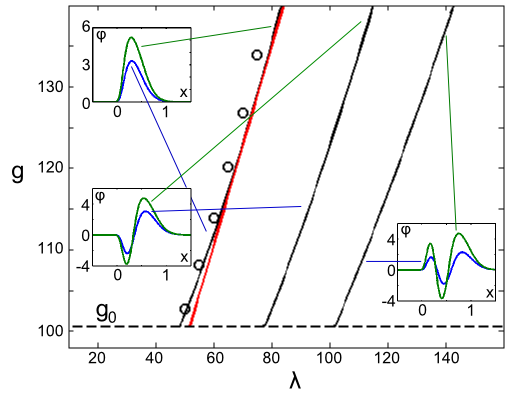
Figure 8: (Color online) Numerically calculated acceleration $g$ for different branches of solutions of Eqs. (27), (28) with the potential $V$ being replaced by its asymptotic $V_{b}$. Circles correspond to the solutions in the full potential $V$. Approximate analytical solution (30) is indicated by dashed line. Insets illustrate solution profiles (asymptotic potential) at different values of the parameter $\lambda$.

It is useful to derive an approximate analytical expression for $g$, which can be done in several ways. First, the variational approach can be applied to the nonlinear problem (27). However, this leads to the rather cumbersome and difficult to understand expressions. More elegant answer, which also matches well our numerical calculations in Fig. 8, can be obtained in the limit of the weak nonlinearity in Eq. (27). This is accomplished by solving Eq. (27) perturbatively. We consider the ground state and assume that in the first order $\phi_{0}$ and $\lambda$ are given by their variational approximations $A\tilde{\phi}_{0}$ and $\tilde{\lambda}_{0}$ found in the linear case, see Eqs. (19), (20). Here $A$ is the constant amplitude to be determined. We also introduce correction to the eigenfunction, $\delta\phi$, and to the eigenvalue, $\delta\lambda=\lambda-\tilde{\lambda}_{0}$, induced by the nonlinearity. Taking $\epsilon$ as a dummy small parameter, we assume $A^{2}\sim\epsilon$, $\delta\phi\sim\epsilon$ and $\delta\lambda\sim\epsilon$. Looking at the integral in Eq. (28) we see that it has order $\epsilon^{2}$, because its value is proportional to $A^{2}$ and it acquires an extra order of smallness due to a small overlap between $\phi_{0}$ and $\psi_{0}$. It means that $g=g_{0}+O(\epsilon^{2})$. The resulting equation for $\delta\phi$ derived from Eq. (27) is

$$(-|d_{2}|\partial^{2}_{\xi}+V(\xi,g_{0})-\tilde{\lambda}_{0})\delta\phi\approx$$

$$\delta\lambda A\tilde{\phi}_{0}-A^{3}\tilde{\phi}_{0}^{3}.$$ (29)

The operator in the left hand side is self-adjoint and singular. Its null-space is given by the linear ground state. Therefore projecting the right-hand side on $\tilde{\phi}_{0}$ we find $\delta\lambda=\sqrt{2}A^{2}$. Substituting $\phi_{0}$ in Eq. (28) with $A\tilde{\phi}_{0}$ and taking into account that inside the integral in Eq. (28) the $\psi_{0}$ can be approximately replaced with its asymptotic $2\sqrt{2q}\exp[-\xi\sqrt{q/d_{1}}]$ we find a relatively simple expression for $g$:

$$g\approx\tilde{g}=g_{0}\cdot\left[1+\frac{\lambda-\tilde{\lambda}_{0}}{q^{9/8}T^{1/4}}\frac{d_{1}^{5/8}}{2|d_{2}|}\sqrt{\frac{\pi}{2}}\left(\frac{15|d_{2}|}{32}\right)^{1/4}\right].$$ (30)

One can see that the above assumption about smallness of the overlap between $\phi_{0}$ and $\psi_{0}$ remains valid provided $q^{-9/8}T^{-1/4}\sim\epsilon$. With $T^{1/4}$ being practically order of $1$, it implies that $q$ should be sufficiently large. Together with the variational approximation for $\tilde{\lambda}_{0}$, see Eq. (23), the above equation agrees very well with numerically calculated dependence of $g$ on $\lambda$ for the ground states, see Fig. 8.

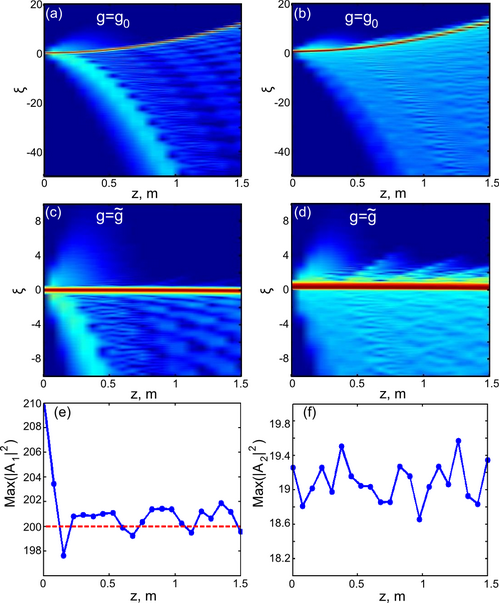
Figure 9: (Color online) Numerical propagation of the lowest bound state within coupled equations (11) and (12) with acceleration $g=g_{0}$, (a) and (b), and $g=\tilde{g}$, (c) and (d). Left column: anomalous GVD component ($A_{1}$), right column: normal GVD component ($A_{2}$). Intensities are plotted in logarithmic scale. (e) and (f): maximum of the intensity of $A_{1}$ and $A_{2}$ components, respectively, along propagation distance. Initial shape for $A_{2}$ was calculated with the approximate potential $V_{b}$ for the soliton parameter $q=100$ and $\lambda=70$ ($\delta\lambda\approx 20$). $A_{1}$ was initialized with the soliton (13) with $q=105$ in order to account for initial radiative losses, see text for more details.

An ultimate method to confirm the validity of our approximate calculations is to take Eqs. (11), (12) in the reference frame moving with acceleration $g=g_{0}$ and with $g=\tilde{g}$ given by Eq. (30), initialize them with the bound state and solve numerically. Then trajectories of the solutions on the $(z,\xi)$-plane should be straight lines in the case of the exactly selected acceleration and parabolic otherwise. Fig. 9 demonstrates the results of this numerical experiment, where intensities of the two components $A_{1}$ and $A_{2}$ are plotted separately. Since initial excitation was taken in a localized form, i.e. without proper account of oscillating tails, one can see that both components emit radiation during propagation. The radiation leakage from the trapped component, $A_{2}$, is small [note logarithmic scale in Figs. 9 (a)-(d)] and does not considerably affect the acceleration of the bound state. More important, however, is the initial outburst of radiation from the soliton component, $A_{1}$. As the result, a noticeable drop in intensity of $A_{1}$ ($\sim 5\%$) is observed during initial stage of soliton propagation, see Fig. 9 (e), while the intensity of the $A_{2}$ component stays practically the same during propagation, see Fig. 9 (f). In order to account for these losses, in the initial condition for $A_{1}$ we have increased the soliton parameter $q$ by $5\%$ with respect to the value used in the calculations of the acceleration $\tilde{g}$. Taking this into account, the Eq. (30) gives a very good approximation for the acceleration of the bound state and, hence, for the rate of the self-frequency shift associated with it, see Figs. 9(c) and (d).

VII Summary

In summary, we have presented the detailed theory of the effect of radiation trapping by the Raman accelerated fiber solitons responsible for formation of the blue wing of the supercontinuum spectra. We demonstrated, that the radiation in the range of the normal GVD is subject to the inertial force, which, together with the soliton induced refractive index change, forms an effective potential well prohibiting the dispersive spreading of the radiation. We have found not only the ground state of the radiation field, but also its excited states, which relevance for the past and ongoing experimental observations is under current investigation. The soliton-radiation bound states move with a constant acceleration in the time-space, while in the spectral domain the peaks corresponding to the two components move in opposite spectral directions (soliton component always gets redder, while the radiation component gets bluer).

In the first part of our theoretical considerations we have assumed that the radiation is linear. In this case we have demonstrated that the continuous blue shift of its frequency happens at the same rate as has been previously calculated for the red shifting solitons Agrawal (2001); Gordon (1986). Considering effects nonlinear in the radiation, we have found that the acceleration of the soliton-radiation bound states increases with the radiation amplitude, which corresponds to larger rates of the self-frequency shift. We have also derived an approximate analytical expression for the latter.

The results presented above pave the way for design of new fiber based soliton frequency converters, which allow for efficient blue frequency shifts of the soliton like state. This removes traditional restriction of the Raman soliton based frequency conversion been directed only towards longer wavelengths. Our results also emphasize that moving dielectric media can be created via nonlinear modulation of the refractive index by the pulse propagating with a speed of light. This creates an interesting testing bed for studies of the effects of light propagation in moving dielectrics, which have generated significant recent interest, see e.g. leon .

- (1)
- Agrawal (2001) G. P. Agrawal, Nonlinear Fiber Optics (Academic Press, 2001), 3rd ed.
- Ranka et al. (2000) J. K. Ranka, R. S. Windeler, and A. J. Stentz, Opt. Lett. 25, 25 (2000).
- Dudley et al. (2002) J. Dudley, X. Gu, L. Xu, M. Kimmel, E. Zeek, P. O’Shea, R. Trebino, S. Coen, and R. Windeler, Opt. Express 10, 1215 (2002).
- Holzwarth et al. (2000) R. Holzwarth, T. Udem, T. W. Hünsch, J. C. Knight, W. J. Wadsworth, and P. S. J. Russell, Phys. Rev. Lett. 85, 2264 (2000).
- Smirnov et al. (2006) S. V. Smirnov, J. D. Ania-Castanon, T. J. Ellingham, S. M. Kobtsev, S. Kukarin, and S. K. Turitsyn, Optical Fiber Technology 12, 122 (2006).
- Hartl et al. (2001) I. Hartl, X. D. Li, C. Chudoba, R. K. Ghanta, T. H. Ko, J. G. Fujimoto, J. K. Ranka, and R. S. Windeler, Opt. Lett. 26, 608 (2001).
- Husakou and Herrmann (2001) A. V. Husakou and J. Herrmann, Phys. Rev. Lett. 87, 203901 (2001).
- Washburn et al. (2002) B. Washburn, S. Ralph, and R. Windeler, Opt. Express 10, 575 (2002).
- Genty et al. (2002) G. Genty, M. Lehtonen, H. Ludvigsen, J. Broeng, and M. Kaivola, Opt. Express 10, 1083 (2002).
- Tartara et al. (2003) L. Tartara, I. Cristiani, and V. Degiorgio, Appl. Phys. B 77, 307 (2003).
- Austin et al. (2006) D. R. Austin, C. M. de Sterke, B. J. Eggleton, and T. G. Brown, Opt. Express 14, 11997 (2006).
- Genty et al. (2004) G. Genty, M. Lehtonen, and H. Ludvigsen, Opt. Express 12, 4614 (2004).
- Hori et al. (2004) T. Hori, N. Nishizawa, T. Goto, and M. Yoshida, J. Opt. Soc. Am. B 11, 1969 (2004).
- Gorbach et al. (2006) A. V. Gorbach, D. V. Skryabin, J. M. Stone, and J. C. Knight, Opt. Express 14, 9854 (2006).
- Frosz et al. (2005) M. Frosz, P. Falk, and O. Bang, Opt. Express 13, 6181 (2005). The authors later claimed that their two frequency quasi-soliton states have had both components in the anomalous GVD range, see Opt. Express 15, 5262 (2007b).
- Nishizawa and Goto (2002a) N. Nishizawa and T. Goto, Opt. Lett. 27, 152 (2002a).
- Nishizawa and Goto (2002b) N. Nishizawa and T. Goto, Opt. Express 10, 1151 (2002b).
- Nishizawa and Goto (2002c) N. Nishizawa and T. Goto, Opt. Express 11, 359 (2002c).
- Cheng et al. (2005) C. Cheng, X. Wang, Z. Fang, and B. Shen, Appl. Phys. B 80, 291 (2005).
- Manassah (1988) J. Manassah, Opt. Lett. 13, 755 (1988).
- Trillo et al. (1988) S. Trillo, S. Wabnitz, E. M. Wright, and G. I. Stegeman, Opt. Lett. 13, 871 (1988).
- Kivshar (1992) Y. Kivshar, Opt. Lett. 17, 1322 (1992).
- Buryak et al. (1996) A. V. Buryak, Y. S. Kivshar, and D. F. Parker, Phys. Lett. A 215, 57 (1996).
- Skryabin and Yulin (2005) D. V. Skryabin and A. V. Yulin, Phys. Rev. E 72, 016619 (2005); A. V. Yulin, D. V. Skryabin, and P. S. J. Russell, Opt. Lett. 29, 2411 (2004).
- Efimov et al. (2005) A. Efimov, A. V. Yulin, D. V. Skryabin, J. C. Knight, N. Joly, F. G. Omenetto, A. J. Taylor, and P. Russell, Phys. Rev. Lett. 95, 213902 (2005); A. Efimov, A. J. Taylor, A. V. Yulin, D. V. Skryabin, and J. C. Knight, Opt. Lett. 31, 1624 (2006).
- Gorbach and Skryabin (2007) A. V. Gorbach and D. V. Skryabin, arXiv:0706.1187 (2007).
- Skryabin et al. (2003) D. V. Skryabin, F. Luan, J. C. Knight, and P. S. J. Russell, Science 301, 1705 (2003).
- Trebino (2000) R. Trebino, Frequency-Resolved Optical Gating: The Measurement of Ultrashort Laser Pulses (Kluwert Academic Publishers, 2000).
- Wai et al. (1990) P. K. A. Wai, H. H. Chen, and Y. C. Lee, Phys. Rev. A 41, 426 (1990).
- Karpman (1993) V. I. Karpman, Phys. Rev. E 47, 2073 (1993).
- Akhmediev and Karlsson (1995) N. Akhmediev and M. Karlsson, Phys. Rev. A 51, 2602 (1995).
- Biancalana et al. (2004) F. Biancalana, D. V. Skryabin, and A. V. Yulin, Phys. Rev. E 70, 016615 (2004).
- Chen and Liu (1976) H.-H. Chen and C.-S. Liu, Phys. Rev. Lett. 37, 693 (1976).
- Gordon (1986) G. Gordon, Opt. Lett. 11, 662 (1986).
- Akhmediev et al. (1996) N. Akhmediev, W. Krolikowski, and A. J. Lowery, Opt. Commun. 131, 260 (1996).
- Aleshkevich et al. (2000) V. Aleshkevich, Y. Kartashov, and V. Vysloukh, Phys. Rev. E 63, 016603 (2000).
- Facão and Parker (2003) M. Facão and D. F. Parker, Phys. Rev. E 68, 016610 (2003).
- (39) A.M. Weiner, R.N. Thurston, W.J. Tomlinson, J.P. Heritage, D.E. Leaird, E.M. Kirschner, and R.J. Hawkins, Opt. Lett. 14, 868 (1989).
- (40) P. Piwnicki and U. Leonhardt, Appl. Phys. B 72, 51 (2001); U. Leonhardt and P. Piwnicki, Phys. Rev. Lett. 84, 822 (2000); U. Leonhardt and P. Piwnicki, Phys. Rev. A 60, 4301 (1999).