From Useful Algorithms for Slowly Convergent Series

to Physical Predictions Based on Divergent Perturbative Expansions

E. Caliceti,^a,∗ M. Meyer–Hermann,^b P. Ribeca,^c A. Surzhykov,^d and U. D. Jentschura^d,∗

^aDipartimento di Matematica, Università di Bologna, 40127 Bologna, Italy
^bFrankfurt Institute for Advanced Study, Max von Laue-Straße 1, 60438 Frankfurt am Main, Germany
^cGesellschaft für Schwerionenforschung (GSI), Planckstraße 1, 64291 Darmstadt
^dMax–Planck–Institut für Kernphysik, Saupfercheckweg 1, 69117 Heidelberg, Germany

This review is focused on the borderline region of theoretical physics and mathematics. First, we describe numerical methods for the acceleration of the convergence of series. These provide a useful toolbox for theoretical physics which has hitherto not received the attention it actually deserves. The unifying concept for convergence acceleration methods is that in many cases, one can reach much faster convergence than by adding a particular series term by term. In some cases, it is even possible to use a divergent input series, together with a suitable sequence transformation, for the construction of numerical methods that can be applied to the calculation of special functions. This review both aims to provide some practical guidance as well as a groundwork for the study of specialized literature. As a second topic, we review some recent developments in the field of Borel resummation, which is generally recognized as one of the most versatile methods for the summation of factorially divergent (perturbation) series. Here, the focus is on algorithms which make optimal use of all information contained in a finite set of perturbative coefficients. The unifying concept for the various aspects of the Borel method investigated here is given by the singularities of the Borel transform, which introduce ambiguities from a mathematical point of view and lead to different possible physical interpretations. The two most important cases are: (i) the residues at the singularities correspond to the decay width of a resonance, and (ii) the presence of the singularities indicates the existence of nonperturbative contributions which cannot be accounted for on the basis of a Borel resummation and require generalizations toward resurgent expansions. Both of these cases are illustrated by examples.

PACS numbers: 11.10Jj, 12.20.Ds, 02.70.-c, 02.60.-x
Keywords: Asymptotic problems and properties,
quantum electrodynamics (specific calculations),
computational techniques,
numerical approximation and analysis.

 ^∗ Corresponding authors. E-mail: caliceti@dm.unibo.it and jentschura@mpi-hd.mpg.de.

1 Background and Orientation

The purpose of this section is that of being a starting point and a reference for the reader. Its contents are organized as follows:

• In Sec. 1.1, a general introduction to convergence acceleration and resummation is provided.

• In Sec. 1.2, some basic terminology is introduced. This terminology is a basis for the general familiarity with the notions that govern the construction of convergence acceleration methods.

The concepts contained in this section constitute to a large extent a prerequisite for the material presented in the following sections.

1.1 Introduction to Convergence Acceleration and Resummation

The basic idea of convergence acceleration is to extract hidden information contained in partial sums of a specific slowly convergent series, and to use that information in order to make, loosely speaking, an educated guess about higher-order partial sums which eventually converge to some limit. In many cases, the “educated guesses” can lead to spectacular numerical results which represent a drastic improvement over a term-by-term summation of the series, even if the series is formally convergent.

Convergence acceleration methods have a long history. E.g., as mentioned of p. ix of Ref. [1], such methods were already used by the Chinese mathematicians Liu Hui (A.D. 263) and Zhu Chongzhi (429—500) for obtaining better approximations to $\pi$. It is thus clear that, at least in rudimentary form, convergence acceleration methods are much older than calculus. Another reference to early successful attempts can be found on pp. 90—91 of a book by Brezinski [2] where it is mentioned that convergence acceleration methods have already been used in 1654 by Huygens and in 1674 by Seki Kowa, the probably most famous Japanese mathematician of his time. Both Huygens and Seki Kowa were trying to obtain better approximations to $\pi$. Huygens used a linear extrapolation scheme which is a special case of what we now call Richardson extrapolation [3], and Seki Kowa used the so-called $\Delta^{2}$ process, which is usually attributed to Aitken [4].

Sequence transformations are principal numerical tools to overcome convergence problems. In this approach, a slowly convergent or divergent sequence $\{s_{n}\}_{n=0}^{\infty}$, whose elements may for instance be the partial sums $s_{n}\;=\;\sum_{k=0}^{n}\,a_{k}$ of an infinite series, is converted into a new sequence $\{s^{\prime}_{n}\}_{n=0}^{\infty}$ with hopefully better numerical properties. Before the invention of electronic computers, mainly linear sequence transformations were used. These matrix transformations compute the elements of the transformed sequence $\{s_{n}^{\prime}\}_{n=0}^{\infty}$ as weighted averages of the elements of the input sequence $\{s_{n}\}_{n=0}^{\infty}$ according to the general scheme $s_{n}^{\prime}\;=\;\sum_{k=0}^{n}\,\mu_{nk}\,s_{k}$. The theoretical properties of such matrix transformations are very well understood [5, 6, 7, 8, 9, 10, 11, 12, 13]. Their main appeal lies in the fact that for the weights ${\mu}_{nk}$ some necessary and sufficient conditions could be formulated which guarantee that the application of such a matrix transformation to a convergent sequence $\{s_{n}\}_{n=0}^{\infty}$ yields a transformed sequence $\{s_{n}^{\prime}\}_{n=0}^{\infty}$ converging to the same limit $s=s_{\infty}$. Theoretically, this regularity is extremely desirable, but from a practical point of view, it is a disadvantage. This may sound paradoxical. However, according to a remark on p. X of Ref. [10], the size of the domain of regularity of a transformation and its efficiency seem to be inversely related. Accordingly, regular linear transformations are in general at most moderately powerful, and the popularity of most linear transformations has declined considerably in recent years.

Modern nonlinear sequence transformations as for instance the $\epsilon$ algorithm [14] and the $\rho$ algorithm [15] or the $\vartheta$ algorithm [16] have largely complementary properties: They are nonregular, which means that that the convergence of the transformed sequence is not guaranteed, let alone to the correct limit. In addition, the theoretical properties of nonlinear transformations are far from being completely understood. Nevertheless, they often accomplish spectacular results when applied to appropriate problems. Consequently, nonlinear transformations now dominate both mathematical research as well as practical applications, as documented in a large number of recent books [17, 18, 19, 20, 21, 10, 22, 23, 24, 25, 1, 26, 27, 28, 29] and review articles [30, 31, 32, 33] on this topic.

We here attempt to present these transformations in both a special context (with a focus on applications) as well as in the general context given by an underlying principle of construction exemplified by the $E$ algorithm. One of the recurrent themes in the construction of sequence transformations is the separation of the series into a partial sum $s_{n}=\sum_{k=0}^{n}a_{n}$ and a remainder $r_{n}=-\sum_{k=n+1}^{\infty}a_{n}$ so that $s_{n}=s+r_{n}$. The remainder term $r_{n}$ is to be approximated by remainder estimates and eliminated from the input data $s_{n}$ by suitable transformations.

We restrict the discussion to the acceleration of sequences. Quite naturally, convergence acceleration methods can be proposed and applied to the pointwise evaluation of partial-wave expansions which occur ubiquitously in physics (see, e.g., Ref. [34, 35]), and to Fourier expansions and other orthogonal series [36]. Here, the sequences are typically composed of the partial sums of the respective expansions. For applications to vector or matrix problems, the reader is referred to the books [25, 37] and numerous articles, e.g. [38, 39], and for applications to numerical quadrature, in particular with respect to oscillatory functions to be integrated over semiinfinite intervals, we refer to the books [40, 28] and several articles which describe corresponding applications, e.g. [41].

Forming a bridge between convergence acceleration and resummation, one may observe that some acceleration algorithms may also be used for the resummation of (mildly) divergent series, but are in general less versatile than the Borel method. The resummed value of a divergent series, which is sometimes called antilimit, can be attributed, according to Euler, to the particular finite mathematical entity whose expansion gives rise to the original series. L. Euler wrote in a letter to Goldbach (1745): ‘Summa cuiusque seriei est valor expressionis illius finitae, ex cuius evolutione illa series oritur,” which may be translated from the Latin language as: “The sum of any given series [whether convergent or divergent] is the value of the specific finite expression whose expansion gave rise to that same series.” One can mention a number of accepted methods for series (re-)summation: e.g., there are averaging processes for oscillatory partial sums like the Césaro method [6] or sophisticated mathematical constructions like zeta function regularization [42], which depend on the availability of closed-form analytic expressions for all terms that need to be summed, and permit the variation of a free parameter (the “argument” of the generalized zeta function) from the physically relevant to a mathematically favourable domain, where the defining series becomes convergent. Later, in order to allow for the determination of the physical property of interest, one performs an analytic continuation of the parameter back to the physical domain. In the same context, one can mention the Mellin-Barnes transform [43].

Divergent series result from any eigenvalue perturbation theory, unless the perturbation is Kato-bounded with respect to the unperturbed Hamiltonian (see Ref. [44]). In particular, the application of simple, “naive” Rayleigh–Schrödinger perturbation theory to a harmonic oscillator with an $x^{4}$ perturbation (where $x$ is the position operator) already leads to a divergent series in higher orders of perturbation theory. While the degree of acceptance of divergent series within the mathematical scientific community underwent some undeserved oscillations during the last two centuries, we are today in the fortunate situation that their properties are routinely investigated and harvested in the context of physical problems that originate from perturbation theory in quantum mechanics and field theory.

One of the most versatile and most relevant resummation algorithms, especially those originating from perturbation theory, is the Borel method [45, 46, 47]. The reason is that many physical divergences are factorial, and for these, the Borel summation is the most powerful one. Already in 1952 Dyson [48] had argued that perturbation expansions in quantum electrodynamics should diverge, and it later turned out [49, 50, 51, 52, 53, 54] that the divergence should be factorial. Also, Bender and Wu [55, 56, 57] demonstrated that Dyson’s speculation was not a mere mathematical sophistication: They proved that the coefficients of the standard Rayleigh–Schrödinger perturbation expansions for the energy eigenvalues of the anharmonic oscillators with anharmonicities $x^{2m}$ with $m\geq 2$ grow at least factorially with the index $n$ as $(m\,n)!$. A new subfield of theoretical physics emerged which is nowadays called large-order perturbation theory (see for example [58, 59, 60] and references therein). Following these works, many other quantum mechanical systems described by perturbation expansions were investigated, and in the overwhelming majority of all cases very similar divergence problems were observed. Moreover, nowadays the factorial divergence of perturbation expansions in quantum field theory and in related disciplines now almost has the status of a law of nature (see for example the discussion in [61]).

The Borel resummation process replaces the divergent series, after analytic continuation of the Borel transform, by a Laplace-type integral, which is sometimes called the Laplace–Borel integral for obvious reasons. A famous ambiguity results in the case of singularities of the transform along the integration contour. In principle, one may imagine three possible interpretations for the ambiguity introduced by the singularities, and it is interesting to remark that all of them might be realized in nature. They are marked here as (i), (ii) and (iii) and will be briefly discussed now. (i) In some cases (e.g., the cubic anharmonic oscillator and the Stark effect), the resummation is achieved by using a complex integration contour, which goes around the singularity on a half circle and leads to an imaginary part for the (resonance) energy eigenvalues of the Hamiltonians under investigation. Of course, the sign of the imaginary part depends on the clockwise or anticlockwise circulation around the pole and cannot be determined on the basis of the purely real perturbation series alone: additional physics input is needed and provided by the very nature of a resonance. These cases find a natural mathematical interpretation via the concept of distributional Borel summability. (ii) There are situations in which the singularities of the Borel transform indicate the presence of further contributions that cannot be obtained on the basis of perturbation theory alone, even if perturbation theory is combined with the most sophisticated resummation methods. Rather, one has to generalize perturbation theory to a resurgent expansion [62, 63, 64, 65]. In some cases, there are subtle cancellations of the imaginary parts created by the singularities of the Borel transform of the perturbation series against explicit imaginary parts of higher-order instanton effects which are characterized by nonanalytic factors, leading to purely real eigenenergies for, e.g., quantum mechanical potentials of the double-well type. The instanton effects, in turn, are decorated again by divergent nonalternating perturbation series, which give to yet further imaginary parts, but these are again compensated by instanton effects of even higher order. The generalized perturbative expansion which entails all of these effects is a so-called resurgent expansion. (iii) One may easily construct mathematical model problems where the correct resummation is achieved by a principal-value prescription for the evaluation of the Borel integral. It has been conjectured that this prescription might be the correct one for a number of physical problems as well. Summarizing, we may state that the ambiguity of the Borel resummation process definitely exists. This ambiguity provides for an interpretation of the Borel transform even in cases where the complete physical answer cannot be obtained on the basis of perturbation theory alone.

The resummation methods allow us to determine eigenenergies and other physical properties on the basis of a finite number of perturbative coefficients alone. One can now even go one step further and observe that, on the one hand, the large-order behaviour of perturbation theory is connected to the underlying perturbative potential or interaction Lagrangian (in the case of a field theory), and yet, on the other hand, the potential also determines the large-coupling expansion for the potential or the field theory under investigation. So, one can even try to guess the large-coupling expansion from a finite number of terms of the weak-coupling perturbative expansion, because these already give an impression of the large-order behaviour. This paradoxical endeavour has been pursued in recent years, in a series of papers, by Suslov [66, 67, 68, 69].

Let us now attempt to form a bridge between convergence acceleration and resummation via sequence transformations, which can be used for the resummation of (mildly) divergent series in addition to their use as convergence accelerators. We recall that the convergence acceleration of the sequence $\{s_{n}\}_{n=0}^{\infty}$ is achieved by eliminating the remainders $r_{n}$ from a necessarily finite set of input data $\{s_{n}\}_{n=0}^{m}$, in order to obtain a better estimate $s^{\prime}_{m}$ to $s$ than the obvious estimate which would be provided by $s_{m}$. Clearly, the “elimination of remainders” is a concept which can be transported to the case of a divergent series. The only difference is that for a convergent series, $r_{n}\to 0$ as $n\to\infty$, whereas for a divergent series, $\lim_{n\to\infty}r_{n}$ does not exist. In some cases, the sequence transformations provide us with numerically favourable, highly efficient algorithms for the computation of the antilimit of the divergent input series, so that they constitute competitive numerical algorithms for the actual computation of the antilimit, which could otherwise only obtained by direct evaluation of the expression which gave rise to the divergent series in the first place, or by the Borel method in connection with Padé approximants for the analytic continuation of the Borel transform. The latter method, although versatile, is numerically less efficient because it entails, at least, the numerical evaluation of the Laplace–Borel integral.

1.2 Mathematical Basis

1.2.1 Special Mathematical Symbols

In order to fix ideas, it is perhaps useful to recall a few mathematical symbols. In particular,

$$\mathbb{N}=\{1,2,3,\ldots\}$$ (1)

denotes the set of positive integers, $\mathbb{N}_{0}=\mathbb{N}\cup\{0\}$ stands for the set $\{0,1,2,\ldots\}$ of nonnegative integers, and

$$\mathbb{Z}=\{0,\pm 1,\pm 2,\ldots\}$$ (2)

is the set of positive and negative integers. Moreover, $\mathbb{R}$ and $\mathbb{C}$ denote the sets of real and complex numbers, respectively.

The symbol $[\mkern-2.5mu[x]\mkern-2.5mu]$ is the integral part of $x\in\mathbb{R}$, i.e., the largest integer $m\in\mathbb{Z}$ satisfying the inequality $m\leq x$.

The nonstandard notation

$$\{s_{n}\}_{n=0}^{\infty}$$ (3)

is used to denote a sequence of elements $s_{n}$ with $n\in\mathbb{N}_{0}$. In this work, we usually assume that every element $s_{n}$ represents the partial sum of an infinite series:

$$s_{n}=\sum_{k=0}^{n}a_{k}\,.$$ (4)

Indeed, such a definition implies that the sequence elements $s_{-1},s_{-2},s_{-3},\ldots$ with negative indices are empty sums and thus equal to zero.

As just indicated, empty sums are always interpreted as zero:

$$\sum_{k=m}^{n}\,a_{k}\;=\;0\,,\qquad\text{if}\quad m>n\,.$$ (5)

Similarly, an empty product is always interpreted as one:

$$\prod_{k=m}^{n}\,a_{k}\;=\;1\,,\qquad\text{if}\quad m>n\,.$$ (6)

Let $f(z)$ and $g(z)$ be two functions defined on some domain $D$ in the complex plane and let $z_{0}$ be a limit point of $D$, possibly the point at infinity. Then,

$$f(z)\;=\;\mathrm{O}(g(z))\,,\qquad z\to z_{0}\,,$$ (7)

means that there is a positive constant $A$ and a neighborhood $U$ of $z_{0}$ such that

$$|f(z)|\;\leq\;A|g(z)|$$ (8)

for all $z\in U\cap D$. If $g(z)$ does not vanish on $U\cap D$ this simply means that $f(z)/g(z)$ is bounded on $U\cap D$. Similarly,

$$f(z)\;=\;\mathrm{o}(g(z))\,,\qquad z\to z_{0}\,,$$ (9)

means that for any positive number $\epsilon\in\mathbb{R}$ there exists a neighborhood $U$ of $z_{0}$ such that

$$|f(z)|\;\leq\;\epsilon|g(z)|$$ (10)

for all $z\in U\cap D$. If $g(z)$ does not vanish on $U\cap D$ this simply means that $f(z)/g(z)$ approaches zero as $z\to z_{0}$.

1.2.2 Finite Differences

So–called finite difference operators [70, 71] are essential in the construction of sequence transformations. Let us consider a function $f(n)$ defined on the set $\mathbb{N}_{0}$ of nonnegative integers. Then, the forward difference operator $\Delta f(n)$ is defined by

$$\Delta f(n)\;=\;f(n+1)-f(n),\qquad n\in\mathbb{N}_{0}\,.$$ (11)

Higher powers of this operator can be defined recursively:

$$\Delta^{k}f(n)=\Delta[\Delta^{k-1}f(n)]\,,\qquad k\in\mathbb{N}\,,$$ (12)

with $\Delta^{0}f(n)=f(n)$. Apart from the forward difference one may also introduce the shift operator:

$$Ef(n)\;=\;f(n+1)\,,$$ (13)

whose higher powers can again be defined recursively:

$$E^{k}f(n) = E[E^{k-1}f(n)]\;=\;f(n+k),\qquad k\in\mathbb{N}\,,$$ (14)

with $E^{0}f(n)=f(n)$. As seen from definitions (11) and (13), the forward difference $\Delta$ and shift $E$ operators are connected by the relationship

$$\Delta\;=\;E-1\,,$$ (15)

where $1$ is the identity operator. This relationship can be combined with the binomial theorem to give

$$\Delta^{k}f(n)\;=\;(-1)^{k}\,\sum_{j=0}^{k}\,(-1)^{j}\,{\binom{k}{j}}\,f(n+j)\,,\qquad k\in\mathbb{N}_{0}\,.$$ (16)

In the following, we always tacitly assume that in the case of quantities, which depend on several indices like $\mathcal{A}_{k}^{(n)}$, the difference operator $\Delta$ and the shift operator $E$ only act only upon $n$ and not on any other indices: e.g., we have $\Delta\mathcal{A}_{k}^{(n)}=\mathcal{A}_{k}^{(n+1)}-\mathcal{A}_{k}^{(n)}$.

Furthermore, we should clarify the notation for sequences with $f(n)=s_{n}$: The quantity $\Delta s_{n}$ is to be understood as $\Delta s_{n}=s_{n+1}-s_{n}=a_{n+1}$, and we have $\Delta^{2}s_{n}=s_{n+2}-2s_{n+1}+s_{n}=\Delta a_{n+1}=a_{n+2}-a_{n+1}$ and so on [we assume the structure given in Eq. (4) for the $s_{n}$].

1.2.3 Asymptotic Sequences and Asymptotic Expansions

A finite or infinite sequence of functions $\{\Phi_{n}(z)\}_{n=0}^{\infty}$, which are defined on some domain D of complex numbers on which all $\Phi_{n}(z)$ are nonzero except possibly at $z_{0}$, is called an asymptotic sequence as $z\to z_{0}$ if for all $n\in\mathbb{N}_{0}$,

$$\Phi_{n+1}(z)\;=\;\mathrm{o}(\Phi_{n}(z))\,,\qquad z\to z_{0}\,.$$ (17)

The formal series

$$f(z)\sim\sum_{n=0}^{\infty}a_{n}\,\Phi_{n}(z)\,,$$ (18)

which need not be convergent, is called an asymptotic expansion of $f(z)$ with respect to the asymptotic sequence $\{\Phi_{n}(z)\}_{n=0}^{\infty}$ in the sense of Poincaré [72] if, for every $m\in\mathbb{N}_{0}$,

$$f(z)-\sum_{n=0}^{m}a_{n}\,\Phi_{n}(z)\;=\;\mathrm{o}(\Phi_{m}(z))\,,\qquad z\to z_{0}\,.$$ (19)

If such a Poincaré-type asymptotic expansion exists, it is unique, and its coefficients $a_{n}$ can be computed as follows,

$$a_{m}\;=\;\lim_{z\to z_{0}}\;\Bigl{\{}\bigl{[}f(z)-\sum_{n=0}^{m-1}\;a_{n}\Phi_{n}(z)\bigr{]}\,/\,\Phi_{m}(z)\Bigr{\}}\,,\qquad m\in\mathbb{N}_{0}\,.$$ (20)

The particularly important case of an asymptotic expansion with respect to the asymptotic sequence $\{z^{-n}\}_{n=0}^{\infty}$ about $z_{0}=\infty$ has the form of an asymptotic power series in $1/z$,

$$f(z)\;\sim\;\sum_{k=0}^{\infty}\;\alpha_{k}/z^{k}\,.\qquad z\to\infty\,.$$ (21)

In the current article, we will often use the notation

$$f(z)\;\sim\;\sum_{k=0}^{\infty}\alpha_{k}\,z^{k}\,,\qquad z\to 0\,,$$ (22)

for asymptotic expansions or perturbative expansions of a physical quantity $f(z)$ with respect to the asymptotic sequence $\{z^{n}\}_{n=0}^{\infty}$ in the sense of Poincaré.

1.2.4 Remainder Estimates

Let us assume that $\{s_{n}\}_{n=0}^{\infty}$ either converges to some limit $s$, or, if it diverges, can be summed by an appropriate summation method to give $s$. Following [73], this generalized limit $s$ is frequently called antilimit in the case of divergence. In either case, there is a partition of a sequence element $s_{n}$ into the limit or antilimit $s$ and the remainder $r_{n}$ according to

$$s_{n}\;=\;s\,+\,r_{n}$$ (23)

for all $n\in\mathbb{N}_{0}$. If $s_{n}$ is the partial sum

$$s_{n}\;=\;\sum_{k=0}^{n}\,a_{k}$$ (24)

of an infinite series, then the remainder $r_{n}$ obviously satisfies

$$r_{n}\;=\;-\sum_{k=n+1}^{\infty}\,a_{k}\,.$$ (25)

In particular, this implies that the remainders $r_{n}$ are all negative if the series terms $a_{n}$ are all positive.

The dependence of the magnitude of the remainder $r_{n}$ on the index $n$ is a natural measure for the convergence of the sequences or series. Often, it is of considerable interest to analyze the asymptotics of the sequence of remainders $\{r_{n}\}_{n=0}^{\infty}$ as $n\to\infty$. Let us assume that we have found an asymptotic sequence $\{\varphi_{k}(n)\}_{k=0}^{\infty}$ as $n\to\infty$ with $\varphi_{0}(n)=1$ for the function $r_{n}/\omega_{n}$, which is equivalent to identifying some dominant part (leading term) $\omega_{n}$ of $r_{n}$ with respect to the asymptotic sequence $\{\varphi_{k}(n)\}_{k=0}^{\infty}$. We call $\omega_{n}$ the remainder estimate. In particular, this means that the remainder term $r_{n}$ can be expanded asymptotically according to

$$r_{n}/\omega_{n}\;\sim\;\sum_{k=0}^{\infty}\,c_{k}\,\varphi_{k}(n)\,,\qquad n\to\infty\,.$$ (26)

Sequences of remainder estimates $\{\omega_{n}\}_{n=0}^{\infty}$ will be of considerable importance in this report. The reason is that it is often possible to obtain at least some structural information about the behavior of the dominant term of a remainder $r_{n}$ as $n\to\infty$. It will become clear later that convergence acceleration or summation methods, which explicitly utilize the information contained in the remainder estimates $\{\omega_{n}\}_{n=0}^{\infty}$, frequently lead to efficient algorithms.

1.2.5 Types of Convergence

The ideas of “linear” and “logarithmic” convergence turn out to be very useful concepts when analyzing the types of convergence of series, and are used very often in the literature on convergence acceleration. They are recalled in the current section.

We observe that the behaviour of the remainder (25) as a function of $n$ is a natural measure for the rate of convergence of the series. In this subsection, therefore, we discuss how different types of behaviour of the $r_{n}$ at $n\rightarrow\infty$ may be used to classify the types of convergence of a particular sequence. In order to perform such a classification, we write

$$\lim_{n\to\infty}\;\frac{s_{n+1}-s}{s_{n}-s}\;=\;\lim_{n\to\infty}\;\frac{r_{n+1}}{r_{n}}\;=\;\rho\,,$$ (27)

where, of course, we assume that the sequence $\{s_{n}\}_{n=0}^{\infty}$ converges to some limit $s$. If, in this equation, $0<|\rho|<1$, we say that the sequence $\{s_{n}\}_{n=0}^{\infty}$ converges linearly, if $\rho=1$ holds, we say that this sequence converges logarithmically, and if $\rho=0$ holds, we say that it converges hyperlinearly. Moreover, $|\rho|>1$ implies that the sequence $\{s_{n}\}_{n=0}^{\infty}$ diverges.

In Ref. [74], it has been shown that if the terms $a_{k}$ of a convergent series are all real and have the same sign, then for $s_{n}=\sum_{k=0}^{n}a_{k}$, we can establish a connection between the remainder $r_{n}$ and the series term $a_{n}$ as follows,

$$\lim_{n\to\infty}\;\frac{r_{n+1}}{r_{n}}\;=\;\lim_{n\to\infty}\;\frac{a_{n+1}}{a_{n}}\;=\;\rho\,.$$ (28)

Effectively, this means that we can replace in the fraction $r_{n+1}/r_{n}$ each of the $r_{n}$ by $\Delta s_{n}$,

$$\lim_{n\to\infty}\;\frac{r_{n+1}}{r_{n}}\;=\;\lim_{n\to\infty}\;\frac{\Delta s_{n+1}}{\Delta s_{n}}\;=\;\rho\,.$$ (29)

Apart from the particular case of the real and nonalternating $a_{n}$, Eq. (29) can be also applied to arbitrary hyperlinearly and linearly convergent real sequences [10].

We are ready now to illustrate the application of Eq. (27) for the classification of the (type of) convergence of some particular series. To this end, let us start from the Riemann zeta function, defined by a Dirichlet series as given in Ref. [75],

$$\zeta(z)\,=\,\sum\limits_{n=0}^{\infty}\frac{1}{(n+1)^{z}}\,.$$ (30)

We would like to determine the type of convergence of this series for a particular case of $z$ = 2. For this case, the reminder (25) reads:

$$r_{n}=-\sum\limits_{k=n+1}^{\infty}\frac{1}{(k+1)^{2}}\,.$$ (31)

By applying the Euler–Maclaurin formula [see, e.g., Eqs. (2.01)—(2.02) on p. 285 of Ref. [76]] to the right side of this expression, we find the leading and the first sub–leading asymptotics of the reminder $r_{n}$,

$$r_{n}\sim-\frac{1}{n+2}-\frac{1}{2(n+2)^{2}}+\sum_{j=1}^{\infty}(-1)^{j}\,\frac{B_{2j}}{(n+2)^{2j+1}}\,,\qquad n\to\infty\,.$$ (32)

Here, $B_{2j}$ is a Bernoulli number [p. 281 of Ref. [76]]. Together with Eq. (27), this immediately implies that the series (30) at $z$ = 2 converges logarithmically, i.e. $\rho=1$ for $n\to\infty$.

A more elaborate example concerns the convergence properties of the alternating series with partial sums:

$$s_{n}=\sum\limits_{k=0}^{n}\frac{(-1)^{k}}{(k+1)^{2}}\,,\qquad\lim_{n\to\infty}s_{n}=\frac{\pi^{2}}{12}\,.$$ (33)

This series is similar to the Dirichlet series for the zeta function $\zeta(2)$, but is strictly alternating in sign. The fact that it converges to $\pi^{2}/12$ is shown, for example, in Sec. 2.2 of Ref. [77]. Via a somewhat rather lengthy calculation, we find for $n\to\infty$:

$$r_{n}=-\sum\limits_{k=n+1}^{\infty}\frac{(-1)^{k}}{(k+1)^{2}}\sim\frac{(-1)^{n}}{2}\,\left(\frac{1}{n^{2}}-\frac{3}{n^{3}}+\frac{6}{n^{4}}-\frac{9}{n^{5}}+{\rm O}(n^{-6})\right)\,.$$ (34)

By inserting this reminder into Eq. (27), we obtain that $\rho=-1$. This means that while $|\rho|=1$, we have $\rho\neq 1$ and so the series is not logarithmically convergent. In this contribution, we will refer to convergent series with remainder terms $r_{n+1}/r_{n}\to-1$ for $n\to\infty$ (i.e., series with $\rho=-1$) as alternating marginally convergent series.

So far, we have discussed the application of the remainder estimates for the classification of the convergence of a particular single sequence. The estimates $r_{n}$, however, can be also be applied to compare the rate of convergence of two different series. To this end, let us assume that two sequences $\{s_{n}\}_{n=0}^{\infty}$ and $\{s^{\prime}_{n}\}_{n=0}^{\infty}$ both converge to the same limit $s$. We shall say that the sequence $\{s^{\prime}_{n}\}_{n=0}^{\infty}$ converges more rapidly than $\{s_{n}\}_{n=0}^{\infty}$ if

$$\lim_{n\to\infty}\;\frac{s^{\prime}_{n}-s}{s_{n}-s}\;=\;\lim_{n\to\infty}\;\frac{r^{\prime}_{n}}{r_{n}}\;=\;0\,.$$ (35)

A further natural question is whether one can replace in Eq. (35) $r_{n}$ by $\Delta s_{n}$ and $r^{\prime}_{n}$ by $\Delta s^{\prime}_{n}$, in analogy to Eq. (29):

$$\lim_{n\to\infty}\;\frac{s^{\prime}_{n+1}-s^{\prime}_{n}}{s_{n+1}-s_{n}}\;=\;\lim_{n\to\infty}\;\frac{\Delta s^{\prime}_{n}}{\Delta s_{n}}\;=\;0\,.$$ (36)

Note that in typical cases, the quantity $s^{\prime}_{n+1}-s^{\prime}_{n}$ which may result from the application of a sequence transformation to $\{s_{n}\}_{n=0}^{\infty}$ cannot simply be replaced by some known term $a_{n}$.

It seems (see Ref. [31]) that the equivalence of (35) and (36) cannot be established universally without making some explicit assumptions about how fast the sequences $\{s_{n}\}_{n=0}^{\infty}$ and $\{s^{\prime}_{n}\}_{n=0}^{\infty}$ approach their common limit $s$. In particular, if $\{s_{n}\}_{n=0}^{\infty}$ converges linearly, then the transformed series $\{s^{\prime}_{n}\}_{n=0}^{\infty}$ can converge more rapidly only if it converges at least linearly or even faster. We can always write

$$\frac{\Delta s^{\prime}_{n}}{\Delta s_{n}}\;=\;\frac{s^{\prime}_{n+1}-s^{\prime}_{n}}{s_{n+1}-s_{n}}\;=\;\frac{s^{\prime}_{n}-s}{s_{n}-s}\;\frac{[(s^{\prime}_{n+1}-s)\,/\,(s^{\prime}_{n}-s)]\,-\,1}{[(s_{n+1}-s)\,/\,(s_{n}-s)]\,-\,1}\;=\;\frac{r^{\prime}_{n}}{r_{n}}\;\frac{r^{\prime}_{n+1}/r^{\prime}_{n}\,-\,1}{r_{n+1}/r_{n}-\,1}\,.$$ (37)

Let us assume now that both $\{s^{\prime}_{n}\}_{n=0}^{\infty}$ as well as $\{s_{n}\}_{n=0}^{\infty}$ fulfill Eq. (29) with limits $\rho^{\prime}$ and $\rho$. We can then write

$$\lim_{n\to\infty}\frac{\Delta s^{\prime}_{n}}{\Delta s_{n}}\;=\;\lim_{n\to\infty}\frac{r^{\prime}_{n}}{r_{n}}\,\frac{\rho^{\prime}-1}{\rho-1}\,.$$ (38)

The equivalence of (35) and (36) immediately follows under the assumptions made, which include the linear convergence of the input series (this ensures $\rho\neq 1$). If, however, $\{s_{n}\}_{n=0}^{\infty}$ converges logarithmically, the denominator of the second term on the right-hand side of Eq. (38) approaches zero as $n\to\infty$. In this case, some additional assumptions about the rate of convergence of $\{s^{\prime}_{n}\}_{n=0}^{\infty}$ to $s$ have to be made.

Finally, we should perhaps remark that the analogous terminology of “exponential” and “algebraic” convergence (instead of “linear” and “logarithmic” convergence) is often used in both the physical as well as the mathematical literature, in particular in situations where the “convergent entities” are different from partial sums of a series. An example would be the rate of convergence of iterative solutions to dynamical problems.

1.2.6 Stieltjes Functions and Stieltjes Series

Stieltjes series are, roughly speaking, paradigmatic examples of asymptotic series for which it is possible to find remainder estimates. These estimates characterize the remainder after the calculation of a partial sum and can be used for the construction of sequence transformations which profit from the additional information contained in the remainder estimates (see, for example, Section II in [78] and references therein).

Specifically, a function $F(z)$ with $z\in\mathbb{C}$ is called a Stieltjes function if it can be expressed as a Stieltjes integral according to

$$F(z)\;=\;\int_{0}^{\infty}\,\frac{\mathrm{d}\Phi(t)}{1+zt}\,,\qquad|\arg(z)|<\pi\,.$$ (39)

Here, $\Phi(t)$ is a bounded, nondecreasing function taking infinitely many different values on the interval $0\leq t<\infty$. Moreover, the moment integrals

$$\mu_{n}\;=\;\int_{0}^{\infty}\,t^{n}\,\mathrm{d}\Phi(t)\,,\qquad n\in\mathbb{N}_{0}\,,$$ (40)

must be positive and finite for all finite values of $n$. If we insert the geometric series $1/(1+x)=\sum_{\nu=0}^{\infty}(-x)^{\nu}$ into the integral representation (39) and integrate term-wise using (40), we see that a Stieltjes function $F(z)$ can be expressed by its corresponding Stieltjes series:

$$F(z)\;=\;\sum_{\nu=0}^{\infty}\,(-1)^{\nu}\,\mu_{\nu}\,z^{\nu}\,.$$ (41)

Whether this series converges or diverges depends on the behavior of the Stieltjes moments $\mu_{n}$ as $n\to\infty$.

If we insert the relationship

$$\sum_{\nu=0}^{n}\ (-x)^{\nu}\;=\;\frac{1}{1+x}\,-\,\frac{(-x)^{n+1}}{1+x}$$ (42)

for the partial sum of the geometric series into the integral representation (39), we see that a Stieltjes function can be expressed as a partial sum of the Stieltjes series (41) plus a truncation error term which is given as an integral (see for example Theorem 13-1 of [31]):

$$F(z)\;=\;\sum_{\nu=0}^{n}\,(-1)^{\nu}\,\mu_{\nu}\,z^{\nu}\,+\,(-z)^{n+1}\,\int_{0}^{\infty}\,\frac{t^{n+1}\mathrm{d}\Phi(t)}{1+zt}\,,\qquad|\arg(z)|<\pi\,.$$ (43)

Moreover, the truncation error term in (43) satisfies, depending upon the value of $\theta=\arg(z)$, the following inequalities (see for example Theorem 13-2 of [31]):

$$\left|(-z)^{n+1}\,\int_{0}^{\infty}\,\frac{t^{n+1}\mathrm{d}\Phi(t)}{1+zt}\right|\;\leq\;\begin{cases}\mu_{n+1}\,|z^{n+1}|\,,&\qquad|\theta|\leq\pi/2\,,\\[8.61108pt] \mu_{n+1}\,\left|\displaystyle\frac{z^{n+1}}{\sin(\theta)}\right|\,,&\qquad\pi/2<|\theta|<\pi\,.\end{cases}$$ (44)

Notice that the expression $\mu_{n+1}\,|z^{n+1}|$ emerges as a natural remainder estimate for the partial sum $\sum_{\nu=0}^{n}\,(-1)^{\nu}\,\mu_{\nu}\,z^{\nu}$ of the input series. This observation will later be used in Sec. 2.2.3 for the construction of a special class of sequence transformations. Detailed discussions of the properties of Stieltjes series and their special role in the theory of summability can be found in Chap. 8.6 of [20] or in Chap. 5 of [27].

2 Sequence Transformations

In the current section, sequence transformations are introduced and discussed in several steps. The goal is both to introduce basic notions connected with the construction of convergence accelerators, and to enable the reader to read and understand further, more specialized literature sources.

• In Sec. 2.1, an overview of some of the most common convergence acceleration methods is given, and the reader is presented with a crude quick-start guidance for the choice of suitable convergence acceleration methods.

• In Sec. 2.2, selected convergence acceleration methods are discussed. Some of these profit from the availability of explicit remainder estimates and can sometimes lead to quite spectacular numerical results.

• In Sec. 2.3, the methods are applied to a number of concrete computational problems, for illustrative purposes. The examples concern both straightforward applications of some of the methods as well as more sophisticated cases, where methods have to combined in an adaptive way.

The Chapter thus provides both abstract as well as very concrete information regarding convergence accelerators.

2.1 Quick Start

As a general preamble, it should be noticed that, as everything comes at a price, there is unfortunately no magic method working in all situations: a famous proof in Ref. [79] shows that a universal transformation accelerating all numerical sequences cannot exist, even if we restrict our attention to convergent sequences, neglecting the divergent case.

No matter which convergence acceleration method is finally selected for a particular problem at hand, some practical effort is always necessary to get the best results: on the one hand, a straightforward usage of the algorithms presented in this review, in the sense of computational recipes, can often lead to misleading and nonsensical numerical results; on the other hand, quite spectacular results can often be achieved if careful use is made of all the available information. A two-step procedure should be followed: before starting the actual numerical investigations the known theoretical results should always be reviewed, to understand if by chance the problem at hand satisfies the applicability conditions of one or more of the existing methods. Only if the answer to this question is negative the user should try out some algorithms blindly, and even in this case a preliminary critical assessment of the nature of the problem can often help in immediately ruling out a number of methods. To illustrate these points, we lay out a possible rough guidance for choosing and implementing the best sequence acceleration method among those which are presented in in the rest of the chapter. A much more complete (and interactive) version of this decision grid can be found in the form of computer program named HELP as introduced and discussed in Ref. [25]. Here, we attempt to present a rather compact discussion.

Before we turn our attention to specific cases, let us mention that it is possible to divide many of the algorithms discussed in the literature into two classes. In the case of “more traditional methods”, an assumption about the mathematical structure of the remainder term $r_{n}$ is implicitly coded into the algorithm. The algorithm is constructed to eliminate remainder terms of a specific structure step by step. The terminology is that the sequence transformation is exact for a specific subset of input series. In the case of “modern nonlinear sequence transformations,” an explicit remainder is coded directly and explicitly into the algorithm: the calculation cannot proceed without the external input of remainder estimates in addition to the terms of the series to be summed. In the case of the modern nonlinear sequence transformations, the algorithm only has to make an assumption regarding the correction term which relates the exact remainder and the remainder estimate, but it is unnecessary to eliminate the entire remainder from the series (only the correction term needs to be dealt with).

For both the “modern” as well as the “traditional” algorithms discussed here, one may indicate a certain unifying concept. Indeed, many of the convergence acceleration methods can be cast into the general structure of the $E$ algorithm (see [80, 81] and Sec. 3.3 of Ref. [31]). By examination of the $E$ algorithm, the following fundamental paradigm, on which all methods seem to be based, can be exposed in a particularly clear fashion: “Make an assumption about the remainder and eliminate it from the partial sums of the series as far as possible.”

In view of the “non-universality theorem” of Ref. [79], the task of finding a suitable acceleration transformation acquires a certain heuristic component. Instead of giving an immediate answer, we should therefore attempt to formulate some useful questions which should be asked first:

• Is a remainder estimate $\omega_{n}$ for the remainder term $r_{n}$ known, or is no such information available? In the first case, one has the option of using one of the nonlinear sequence transformations discussed here in Secs. 2.2.3 and 2.2.4 and in Secs. 7 and 8 of Ref. [31]. These transformations profit from remainder estimates and make implicit assumptions about the correction term which corrects the remainder estimate in the direction of the explicit remainder. If no remainder estimate is available, then one only has the option of one of the more traditional methods covered in Secs. 2.2.1 and 2.2.2, which do not need as input an explicit remainder estimate. Note, however, that the more traditional algorithms nevertheless make assumptions about the mathematical structure of the remainder term: the quality of the results varies strongly depending on the validity of these assumptions, and thus one can generally recommend to try more than one method on a particular given problem.

• Is the convergence of the input series known to be linear or logarithmic, and is the sign pattern of the terms of the input series alternating or nonalternating? If this knowledge is available, then the choice of applicable convergence accelerators can be narrowed down further. Details can be found throughout Chap. 2. In general, the application of convergence accelerators to alternating series is numerically much more stable than to nonalternating series. Furthermore, the acceleration of logarithmic convergence is generally recognized as a more demanding task as compared to the acceleration of linear convergence. However, as discussed in this review, a few rather powerful algorithms are currently available.

• Is it the aim to obtain a specific numerical result for a physical quantity under investigation, e.g., an energy level or a cross section, to the highest accuracy based on a finite number of terms of an input series, or is the goal to develop a high-performance algorithm, e.g., for a special function which is given by an asymptotic series expansion whose terms are known? In the first case, there is no need for a computationally efficient implementation of the acceleration algorithm: typically, a knowledge of its definition is sufficient, and in order to avoid numerical loss in higher transformation orders, one may use multi-precision arithmetic, which is implemented in today’s computer algebra systems (e.g., Ref. [82]) in intermediate steps. E.g., if there is no concern about computational efficiency, then it is possible to directly key the definitions given in Eqs. (96) and (101) into a computer program, without making use of the recursive schemes defined in Eqs. (89) and (90) below. The same applies to prototyping applications for numerical algorithms. In the second case, however, one typically has highly powerful recursive schemes available for the calculation of higher-order transformations which reduce the calculational demand by orders of magnitude. The latter aspect is crucial to the applicability of convergence accelerators. In order to appreciate this aspect, one should remember that it was the discovery of the $\epsilon$ algorithm in Ref. [14] which sparked a huge interest in Padé approximants which in turn constitute a paradigmatic example of a versatile convergence acceleration algorithm.

We can now turn our attention to the actual algorithms which have a certain prominent status among the many methods available from the literature. Here, it is inevitable to name some algorithms which will be defined only in Chap. 2 below. The authors hope that this aspect will not lead to confusion. In general, one may distinguish four cases, according to Eq. (27):

• Linear convergence, alternating series: In this case, a number of methods is available, e.g., the $\epsilon$ algorithm or the (iterated) $\Delta^{2}$ process always lead to some acceleration. These two algorithms are discussed in Secs. 2.2.1 and 2.2.2, respectively. A further possibility is provided by polynomial extrapolation with geometrically convergent interpolation points (see Sec. 2.2.2, Sec. 6.1 of Ref. [31], and p. 6 ff. as well as pp. 36–42 of Ref. [19], and Sec. 3.1 of Ref. [83]). The mentioned algorithms fall into the “traditional” category discussed above, and are by construction exact for model sequences which approximate typical cases of linearly convergent series. Moreover, the acceleration of alternating series typically constitutes a numerically very stable process in higher transformation orders. If a remainder estimate is available, then one may also study the behaviour of special sequence transformations, typically the nonlinear $t$ and $d$, and the $\tau$ and $\delta$ transformations discussed here in Secs. 2.2.3 and 2.2.4 (see also Table 1 in the current review) and in Secs. 7 and 8 of Ref. [31]. Observe, however, that the more traditional algorithms also make special assumptions about the mathematical structure of the remainder terms, and that these may lead to numerically very favourable results if the series matches the corresponding assumptions of the algorithm.

• Linear convergence, nonalternating series: From a theoretical point of view, there is no difference between the cases of linearly convergent, alternating series and linearly convergent, nonalternating series. However, from a practical point of view, the difference is huge: because any convergence accelerator automatically entails the calculation of higher weighted differences of elements of the input series, the calculation of higher-order transformations of a nonalternating series can be a numerically highly unstable process. The following question does not even have to be asked, as it usually penetrates practical considerations immediately: Does the accelerated series converge fast enough to the required accuracy in order to be able to overcome the pileup of numerical loss of precision due to roundoff? If the convergence is fast enough, then the direct application of one of the above mentioned algorithms to the input series is possible. If the roundoff errors pile up too fast, then it becomes necessary to make additional efforts. One possibility is to take the nonalternating series as input to a condensation transformation, to generate an alternating series as a result of the condensation transformation, and then, to take the resulting series as input to an additional second acceleration process: here, variants of the CNC transformation (see Sec. 2.2.6) may be useful.

• Alternating marginally convergent series: If remainder estimates are available, then it is possible to use nonlinear sequence transformations, e.g., the $u$, $d$ and $v$, and the $y$, $\delta$ and $\phi$ transformations (see Sec. 2.2.4 here and Secs. 7 and 8 of Ref. [31]). Only for the alternating case, the $\epsilon$ algorithm (see Sec. 2.2.1) may still lead to some acceleration, but its numerical results in the case of logarithmically convergent series are in general very poor [see also Eq. (58) below].

• Logarithmic convergence, nonalternating series: This is in general the most problematic case, because numerical roundoff almost inevitably piles up in higher transformation orders. If it is possible to clearly discern the mathematical structure of the input series, then it may still be possible to use a one-step convergence acceleration algorithm with good effect. An example would be polynomial extrapolation with interpolation points which are given as inverse powers of the index, if the input series has a corresponding structure (see Sec. 2.2.2, Sec. 6.1 of Ref. [31] and Ref. [19]). Another option is to transform first to an alternating series via a condensation transformation, and to use an efficient accelerator for the resulting alternating series. The latter method leads to variants of the CNC transformation (see Sec. 2.2.6).

The above list of algorithms is incomplete. E.g., the $\vartheta$ algorithm derived in Ref. [16, 19] is known to be quite an efficient accelerator for both linearly convergent as well as logarithmically convergent sequences. In some sense, the $\vartheta$ algorithm has a special status because it cannot be derived as a variant of the $E$ algorithm. As remarked in Sec. 15.5 of Ref. [31], the $\vartheta$ algorithm as well as its iterations ${\cal J}^{(n)}_{k}$ are less robust than the $\epsilon$ and $\rho$ algorithms, and in addition, the $\vartheta$ algorithm is outperformed by nonlinear sequence transformations (notably, the $u$ and $v$ transformations) in many cases of logarithmically convergent sequences. Nevertheless, because of its unique position as a rather robust, and rather universal accelerator, the $\vartheta$ algorithm definitely has to be mentioned in this review (see Sec. 2.2.2). In that sense, and at the risk of some over-simplification, we can say that the $\vartheta$ algorithm interpolates between the rather universally applicable, but moderately powerful $\epsilon$ and $\rho$ algorithms on the one hand and the specialized, but potentially spectacularly powerful nonlinear sequence transformation with remainder estimates on the other hand.

A rather heroic attempt at a universally applicable accelerator is the COMPOS algorithm presented in [25], which consists of many base sequence transformations (up to $9$ in the original implementation) being performed in parallel. The results of the parallel transformations are sorted according to their apparent convergence via the SELECT algorithm (here, the apparent convergence is given by the relative change in the numerical values of the transforms as the order of the transformation is increased). The output sequences (or a subset of them) are COMPOSed by making use of the $E$-algorithm. It has been proven that if one of the base transformation accelerates a sequence, then also the composite transformation will accelerate the same sequence. In addition, the speed of convergence of the composite transformation is usually not much worse than that of the best base transformation for the sequence (and can even be better if many of the base transformations converge quickly). A not so serious criticism of the COMPOS algorithm is based on the observation that the algorithm fails when one or more of the base transformations converge quickly to a wrong answer. The interested reader can consult [25] for further details, but this drawback is of course shared by un-composed transformations as well. A rather serious drawback of the COMPOS algorithm, however, lies in the computational effort implied by the necessity to perform the initial transformations in parallel: if the goal is to develop an efficient numerical algorithm for a mathematical entity defined by a slowly convergent series by implementing a convergence accelerator, then the computation overhead implied by the COMPOS algorithm can be quite severe.

Hints concerning the actual implementation of the methods discussed here can be found, e.g., in Refs. [31, 84] concerning sequence transformations, including the $\epsilon$ and the $\rho$ algorithms, and in Ref. [25] concerning a number of rather sophisticated algorithms, including COMPOS. Finally, let us remark that a complete implementation of the CNC transform, adapted to the computation of the Lerch transcendent, is available for download [85]. With these preliminaries being discussed, let us know go in medias res.

2.2 Selected Methods

2.2.1 Padé Approximants

As already discussed in Section 1.2.3, in many problems of theoretical physics, a physical quantity $f(z)$ can be presented in terms of its asymptotic or perturbation expansion (22) with respect to the asymptotic power series $\{z^{n}\}_{n=0}^{\infty}$. Often, the convergence problems with such power series can be overcome by making use of the Padé approximants. The literature on Padé approximants is abundant. A classic reference is [17], and further volumes (Refs. [86, 87, 20, 27]) provide additional valuable information. From among the many other articles that deal with the subject, we only mention Refs. [88, 89, 90, 91, 20, 92, 27, 93]. A Padé approximant produces a rational approximation to the original input series which is given by the ratio of two polynomials. For instance, the $[l/m]$ Padé approximant to a power series (22)

$$f(z)=\sum_{k=0}^{\infty}\alpha_{k}\,z^{k}$$ (45)

is given by the ratio of two polynomials $P_{l}(z)$ and $Q_{m}(z)$ of degree $l$ and $m$, respectively:

$$[l/m]_{f}(z)\;=\;\frac{P_{l}(z)}{Q_{m}(z)}\;=\;\frac{p_{0}+p_{1}\,z+\ldots+p_{l}\,z^{l}}{q_{0}+q_{1}\,z+\ldots+q_{m}\,z^{m}}\;,$$ (46)

where $q_{0}$ is canonically fixed to a unit value. The polynomials $P_{l}(z)$ and $Q_{m}(z)$ are constructed so that the Taylor expansion of the Padé approximant (46) agrees with the original input series up to the order of $l+m$

$$f(z)\;-\;[l/m]_{f}(z)\;=\;\sum_{k=0}^{\infty}\alpha_{k}\,z^{k}-[l/m]_{f}(z)\;=\;{\rm O}(z^{l+m+1})\,.$$ (47)

This equation, therefore, can be used in order to find the coefficients of the polynomials $P_{l}(z)$ and $Q_{m}(z)$. That is, by comparing coefficients at the same orders of $z$ and assuming $q_{0}$ = 1, one gets a system of $l+m+1$ coupled equations to determine $p_{0},p_{1},q_{1},p_{2},q_{2},\dots$. In most cases it is quite inconvenient to solve this system of equations. A more attractive recursive prescription for the evaluation of Padé approximants is the $\epsilon$-algorithm given by the formulas [14, 31]

$$\epsilon_{-1}^{(n)} = 0\,,\qquad\epsilon_{0}^{(n)}\;=\;s_{n}\,,$$ (48a)

$$\epsilon_{k+1}^{(n)} = \epsilon_{k-1}^{(n+1)}\;+\;1/[\epsilon_{k}^{(n+1)}-\epsilon_{k}^{(n)}]$$ (48b)

for $n,k\in\mathbb{N}_{0}$. For the case when the input data $\epsilon_{0}^{(n)}=s_{n}$ are the partial sums

$$s_{n}\;=\;\sum_{k=0}^{n}\;a_{k}\;=\;\sum_{k=0}^{n}\;\alpha_{k}\;z^{k}$$ (49)

of the power series Eq. (22), the elements $\epsilon_{2k}^{(n)}$ of the two-dimensional table of transformations produce Padé approximants according to

$$\epsilon_{2k}^{(n)}\;=\;[n+k/k]_{f}(z)\,.$$ (50)

The odd elements of the table of transformations $\epsilon_{2j+1}^{(n)}$ (with $j\in\mathbbm{N}_{0}$) are only auxiliary quantities.

The above formulas would not be meaningful without some interpretation. First, we observe that the Padé approximant $[n/0]_{f}(z)$ exactly reproduces the partial sum $s_{n}$ of the input series. For the computation of $[n+1/1]_{f}(z)$, we need $s_{n}$, $s_{n+1}$ and $s_{n+2}$ (two elements in addition to the start element $s_{n}$), and therefore the approximant $[n+1/1]_{f}(z)$ constitutes a transformation of second order. In order to compute the Padé approximant $[n+k/k]_{f}(z)$, we need the elements $s_{n+1},\dots,s_{n+2k}$ in addition to $s_{n}$, and the transformation therefore is of order $2k$.

In Eq. (4.3-2) of Ref. [31], it is remarked that the elements of the $\epsilon$ table connected by the formula (48b) form a rhombus in the $(n,k)$ plane. The general paradigm of the $\epsilon$ algorithm is to use the recursive scheme in order to increase the transformation order as far as possible for a given number of elements of the input sequence. If the elements $s_{n},\dots,s_{n+m}$ are known, then highest-order transform which can be calculated is $\epsilon_{2[\mkern-2.5mu[m/2]\mkern-2.5mu]}^{(n)}$. Rather sophisticated techniques are available for a computationally efficient implementation of recursive schemes like the one given in Eq. (48). Typically, in most cases the surprising conclusion is that a single, one-dimensional array of elements is sufficient in order to perform the transformation, whereas the structure of the recursion relation would otherwise suggest that at least a two-dimensional array is needed. Details on the latter point can be found, e.g., in Secs. 4.3, 7.5 and 10.4 of Ref. [31].

An important point, which has certainly not escaped the reader’s attention, is that for $z=1$, the two forms of the input data in Eq. (49) become equivalent with $a_{k}=\alpha_{k}$, and in this case, the Padé approximant is nothing but a (nonlinear) sequence transformation of the input series $\{s_{n}\}_{n=0}^{\infty}$. In fact, the $\epsilon$ algorithm makes no difference between input data which are partial sums of a power series of term $\alpha_{k}z^{k}$ and partial sums of a simple input series of terms $a_{k}$. It might also be helpful to remark that the $\epsilon$ algorithm is exact for sequences of the form (see e.g. Ref. [94])

$$s_{n}=\sum_{j=0}^{k-1}c_{j}\,\lambda^{n}_{j}\,,\qquad|\lambda_{0}|>|\lambda_{1}|>\ldots>|\lambda_{k-1}|\,,$$ (51)

which is a terminating series composed of, loosely speaking, “linearly convergent terms” (if $|\lambda_{0}|<1$).

It is time now for a very brief historical detour. The modern history of convergence started with the seminal paper [73], in which the Shanks transformation $e_{k}(s_{n})$ was introduced. This transformation later turned out to be equivalent to the calculation of Padé approximants. In fact, the transformation $e_{k}(s_{n})$ and the $\epsilon$ algorithm are related by [see, e.g., Eq. (4.2-2) of Ref. [31]]:

$$\epsilon^{(n)}_{2k}=e_{k}(s_{n})\,.$$ (52)

It was the article [14] which elucidated that a highly efficient recursive scheme for the calculation of the approximants $e_{k}(s_{n})$ can be devised. The Shanks transformation, from our point of view, constitutes a way of expressing a diagonal Padé approximant $[n+k/k]_{f}(z)$ to a function.

The entries of the $\epsilon$ table with odd lower index satisfy

$$\epsilon_{2j+1}^{(n)}\;=\;\frac{1}{e_{j}(\Delta s_{n})}\,=\;\mathrm{O}(z^{-n-2j-1}).$$ (53)

Let us interpret this relation. We have assumed that the sequence composed of the $s_{n}$ can be written as $\left\{\sum_{k=0}^{n}\alpha_{k}\,z^{k}\right\}_{n=0}^{\infty}$. The sequence composed of the $\Delta s_{n}$ is thus $\left\{\alpha_{n+1}\,z^{n+1}\right\}_{n=0}^{\infty}$. The expression for the $n$th sequence element $\alpha_{n+1}\,z^{n+1}$ can be written as the partial sum of a power series,

$$\Delta s_{n}=\alpha_{0}+\sum_{k=0}^{n}\left(\alpha_{k+1}\,z^{k+1}-\alpha_{k}\,z^{k}\right)\,.$$ (54)

As $n\to\infty$, all coefficients of this power series vanish, and the function $\Delta s_{\infty}$ is zero. The quantities $e_{j}(\Delta s_{n})$ can thus be identified as $[n+j/j]$-Padé approximants to a specific function defined by a power series whose partial sums are given by Eq. (54), and since all coefficients of that function vanish as $n\to\infty$, we have $e_{j}(\Delta s_{n})=\mathrm{O}(z^{n+2j+1})$ by construction of the Padé approximant.

In writing expressions like $\epsilon^{(n)}_{2k}$ or $e_{k}(s_{n})$, we encounter a certain problem in the notation. Indeed, $n$ is an index which is normally associated to a specific element $s_{n}$, and once $n$ is fixed, $s_{n}$ is fixed also. Here, as in many other literature sources in the field, $n$ is often used in a double meaning: first, to indicate the starting element of a transformation (fixed index), and second, to indicate all the sequence elements $s_{m}$ with $m\in\{n,\dots,n+j\}$ which are needed in order to construct a transformation of a specified order $j$. Observe that in order to calculate $e_{k}(s_{n})$, the elements $s_{n},\dots,s_{n+2k}$ are needed, as $e_{k}(s_{n})$ is a transformation of order $2k$. The simple notation $e_{k}(s_{n})$ might otherwise suggest that the transformation takes as input only the element $s_{n}$, and this is simply not the case. However, a certain compromise between the exactness and completeness of a notation and its compactness and practical usefulness must be found, and the notation $e_{k}(s_{n},\dots,s_{n+2k})$ undeniably looks rather clumsy. The customary notation $e_{k}(s_{n})$ is thus being adopted here.

Let us briefly review the behaviour of the $\epsilon$ algorithm for a number of model series. We follow Ref. [94]. For a linearly convergent series with remainders

$$s_{n}\sim s+\sum_{j=0}^{\infty}c_{j}\,\lambda_{j}^{n}\,,\qquad 1>\lambda_{0}>\lambda_{1}>\dots>0\,,\qquad n\to\infty\,,$$ (55)

the $\epsilon$ algorithm has the following behaviour as $n\to\infty$ for fixed $k$,

$$\epsilon^{(n)}_{2k}\sim s+c_{k}\left(\frac{\Pi_{j=0}^{k-1}(\lambda_{k}-\lambda_{j})}{\Pi_{j=0}^{k-1}(1-\lambda_{j})}\right)^{2}\,\lambda^{n}_{k}\,,\qquad n\to\infty\,.$$ (56)

The $\epsilon$ algorithm thus accelerates convergence according to the definition in Eq. (35) because $(\lambda_{k}/\lambda_{0})^{n}\to 0$ for $n\to\infty$ (we have $\lambda_{k}<\lambda_{0}$ by assumption). For a marginally convergent sequence with strictly alternating remainders,

$$s_{n}\sim s+(-1)^{n}\sum_{j=0}^{\infty}\frac{c_{j}}{(\beta+n)^{j+1}}\,,\qquad\beta>0\,,\qquad n\to\infty\,,$$ (57)

the following estimate has been found in Ref. [94] for fixed $k$, assuming $c_{0}\neq 0$,

$$\epsilon^{(n)}_{2k}\sim s+\frac{(-1)^{n}(k!)^{2}}{2^{2k}\,(\beta+n)^{2k+1}}c_{0}\,.\quad n\to\infty\,.$$ (58)

Also here, the $\epsilon$ algorithm accelerates convergence because $(\beta+n)/(\beta+n)^{2k+1}\to 0$ for $n\to\infty$ for $k>0$. However, the expression $(k!)^{2}$ in the numerator suggests that the $\epsilon$ algorithm encounters problems when one tries to increase the order of the transformation $k$ for given index $n$ of the start element of the transformation. For monotone (nonalternating) series,

$$s_{n}\sim s+\sum_{j=0}^{\infty}\frac{c_{j}}{(\beta+n)^{j+1}}\,,\qquad\beta>0\,,\qquad n\to\infty\,,$$ (59)

the $\epsilon$ algorithm is unable to accelerate convergence,

$$\epsilon^{(n)}_{2k}\sim s+\frac{c_{0}}{(k+1)\,(\beta+n)}\,,\quad n\to\infty\,.$$ (60)

Indeed, the convergence theory of Padé approximants is quite well developed [17, 27], and the above examples are provided only for illustrative purposes.

Besides the model series discussed above, we would like to recall briefly the convergence and acceleration results obtained with the $\epsilon$ algorithm when applied to two important classes of sequences: totally monotonic and totally oscillating sequences. Here, we start our discussion with totally monotonic sequences $s_{n}$ which by definition have the following property:

$$(-1)^{k}\,\Delta^{k}s_{n}\geq 0\qquad\forall k,n\in\mathbb{N}_{0}\,.$$ (61)

This condition implies that since $s_{n}\geq 0$ (set $k=0$ in Eq. (61)), we have $s_{n}\geq s_{n+1}\geq 0$ (set $k=1$ in Eq. (61)). A totally monotonic sequence converges in such a way that $\forall n$, we have $s_{n}\geq s\geq 0$. Another, equivalent definition of a totally monotonic sequence is possible. Namely, it can be proven that a necessary and sufficient condition that $s_{n}$ is a totally monotonic sequence is given by the existence of a bounded and non-decreasing measure ${\rm d}\alpha(x)$ in $[0,1]$ such that:

$$s_{n}=\int\limits_{0}^{1}x^{n}{\rm d}\alpha(x)\,.$$ (62)

The sequences $s_{n}=\lambda^{n}$ where $0<\lambda<1$ and $s_{n}=1/(n+1)$ are examples of totally monotonic sequences.

The properties of totally monotonic sequences have been discussed in detail elsewhere (see, for example, Refs. [25, 95]). In the present manuscript, we just mention the convergence properties. Namely, it has been proven in [96] that if the $\epsilon$ algorithm is applied to a sequence $s_{n}$ which converges to $s$ and if there exist parameters $a$ and $b$ such that $a\,s_{n}+b$ is a totally monotonic sequence, then it is possible to prove the following properties which ensure the convergence of the Padé approximants given by the $\epsilon$ algorithm to the limit $s$, as both $n$ and/or $k$ are increased. Namely, we have $\forall k$ and $\forall n$ (see p. 89 of Ref. [25]),

$$0\leq a\epsilon_{2k+2}^{(n)}+b\leq a\epsilon_{2k}^{(n)}+b\,,$$ (63a)

$$0\leq a\epsilon_{2k}^{(n+1)}+b\leq a\epsilon_{2k}^{(n)}+b\,,$$ (63b)

$$0\leq a\epsilon_{2k+2}^{(n)}+b\leq a\epsilon_{2k}^{(n+1)}+b\,,$$ (63c)

$$0\leq a\epsilon_{2k+2}^{(n)}+b\leq a\epsilon_{2k}^{(n+2)}+b\,,$$ (63d)

$$\forall k\quad{\rm fixed},\quad\lim_{n\to\infty}\epsilon_{2k}^{(n)}=s\,,$$ (63e)

$$\forall n\quad{\rm fixed},\quad\lim_{k\to\infty}\epsilon_{2k}^{(n)}=s\,.$$ (63f)

As expressed by Theorem 2.23 of Ref. [25], all the columns and all the descending diagonals of the $\epsilon$ algorithm can be used for the acceleration of convergence of a totally monotonic series, provided the input series is a non-logarithmic totally monotonic series. We recall that the $\epsilon$ algorithm is unable to accelerate logarithmic convergence.

In a similar way as for a totally monotonic series, the $\epsilon$ algorithm can also be useful for the summation of totally oscillating series. Sequences of that kind are defined in the following way: a $s_{n}$ is totally oscillating if the sequence $(-1)^{n}s_{n}$ is totally monotonic. Again, it has been proven that if the $\epsilon$ algorithm is applied to a sequence $s_{n}$ which converges to $s$ and if there exists $a$ and $b$ such that $as_{n}+b$ is totally oscillating sequence, then we have $\forall k$ and $\forall n$ according to Ref. [25]:

$$0\leq a\,\epsilon_{2k+2}^{(2n)}+b\leq a\,\epsilon_{2k}^{(2n)}+b\,,$$ (64a)

$$a\,\epsilon_{2k}^{(2n+1)}+b\leq a\,\epsilon_{2k+2}^{(2n+1)}+b\leq 0\,,$$ (64b)

$$a\,\left(\epsilon_{2k}^{(2n+1)}-\epsilon_{2k}^{(2n)}\right)\leq a\,\left(\epsilon_{2k+2}^{(2n+1)}-\epsilon_{2k+2}^{(2n)}\right)\leq 0\,,$$ (64c)

$$0\leq a\left(\epsilon_{2k+2}^{(2n+2)}-\epsilon_{2k+2}^{(2n+1)}\right)\leq a\left(\epsilon_{2k}^{(2n+2)}-\epsilon_{2k}^{(2n+1)}\right)\,,$$ (64d)

$$0\leq a\,\epsilon_{2k+2}^{(2n)}+b\leq a\,\epsilon_{2k}^{(2n+2)}+b\,,$$ (64e)

$$a\,\epsilon_{2k}^{(2n+3)}+b\leq a\,\epsilon_{2k+2}^{(2n+1)}+b\leq 0\,,$$ (64f)

$$\forall k\quad{\rm fixed},\quad\lim_{n\to\infty}\epsilon_{2k}^{(n)}=s\,,$$ (64g)

$$\forall n\quad{\rm fixed},\quad\lim_{k\to\infty}\epsilon_{2k}^{(n)}=s\,.$$ (64h)

2.2.2 Further Convergence Accelerators without Remainder Estimates

The $\epsilon$ algorithm takes as input only the elements of the series to be accelerated. No additional remainder estimates are needed. This property is shared by the $\Delta^{2}$ process, the $\rho$ algorithm, and the $\vartheta$ algorithm, which are discussed in the current subsection.

The $\Delta^{2}$ process is widely applied to the summation of slowly convergent series. It is usually attributed to Aitken [4], but there are indications that it may already have been known to Kummer [97]. Within this process, one makes use of the forward difference operator (11) in order to transform the original sequence $\{s_{n}\}_{n=0}^{\infty}$ into a new sequence $\{\mathcal{A}_{n}\}_{n=0}^{\infty}$, whose elements are defined by:

$$\mathcal{A}_{n}=s_{n}-\frac{\left[\Delta s_{n}\right]^{2}}{\Delta^{2}s_{n}}\,.$$ (65)

The structure of this equation clearly explains why Aitken’s method is called $\Delta^{2}$ method. Before discussing the convergence properties of the transformation (65), we would like to mention that originally Aitken’s process was designed to deal with the model sequence of the following form [4], which is a truncated form of Eq. (51):

$$s_{n}=s+c\,\lambda^{n}\,.$$ (66)

As seen from this equation, each sequence element $s_{n}$ contains two coefficients $c\neq 0$ and $|\lambda|<1$ as well as the limit $s$. The first and the second forward differences of such a sequence read:

$$\Delta s_{n}\;=\;c\,\lambda^{n}\,\left(\lambda-1\right)\,,\qquad\Delta^{2}s_{n}\;=\;c\,\lambda^{n}\,\left(\lambda-1\right)^{2}\,.$$ (67)

By inserting now these relations into Eq. (65), we may easily find:

$$\mathcal{A}_{n}=(s+c\,\lambda)-c\,\lambda=s\,,$$ (68)

which implies that the $\Delta^{2}$ process is exact for the model sequence (66) at every stage. Like any other algorithm of numerical analysis, this method has its own domain of validity. Because the (convergence) properties of the transformation (65) have been discussed in detail elsewhere [18, 19, 10], here we just mention that the $\Delta^{2}$ process (i) accelerates linear convergence and (ii) is regular but not accelerative for logarithmically convergent sequences. This indicates that $\Delta^{2}$ process has similar properties as the $\epsilon$–algorithm but is usually not as powerful as the latter one [31]. One may increase the accelerative power of the Aitken’s method, however, by applying this method iteratively. That is, it is first applied to the original sequence $\{s_{n}\}_{n=0}^{\infty}$, then to the transformed sequence $\{\mathcal{A}_{n}\}_{n=0}^{\infty}$ and so on. The detailed discussion on the iterated $\Delta^{2}$ process is given in the texts by Brezinski and Redivo Zaglia (see pp. 128–131 of Ref. [25]) and Weniger (see pp. 223–228 of Ref. [31]) and, therefore, will be omitted in the present report. Apart from the iterative procedure, moreover, a large number of modifications to the $\Delta^{2}$ algorithm have been presented in Refs. [98, 99, 100] and many others. At the end of a rather brief discussion on the Aitken’s $\Delta^{2}$ method, we shall note that this method has very close connection to the $\epsilon$ algorithm as well as to the Padé approximants. For instance, it immediately follows from the derivation of the sequence transformation $\mathcal{A}_{n}$ via the model sequence (66) that $\mathcal{A}_{n}=\epsilon_{2}^{(n)}=[n+1/1]_{f}(z)$ is effectively a Padé approximant to the input sequence given by $s_{n}=\sum_{k=0}^{n}\alpha_{k}z^{k}$.

Beside the $\Delta^{2}$ process, another very well-known sequence transformation is the $\rho$ algorithm [15], which is exact for logarithmically convergent sequences of the following structure,

$$s_{n}=\frac{sx^{k}_{n}+a_{1}x_{n}^{k-1}+\ldots+a_{k}}{x^{k}_{n}+b_{1}x_{n}^{k-1}+\ldots+b_{k}}\,,\,\qquad k,n\in\mathbb{N}_{0},$$ (69)

where the $x_{n}$ are usually chosen to be $x_{n}=\beta+n$ with $\beta\geq 0$. The $\rho$ algorithm is defined by the scheme

$$\rho_{-1}^{(n)} = 0\,,\qquad\rho_{0}^{(n)}\;=\;s_{n}\,,$$ (70a)

$$\rho_{k+1}^{(n)} = \rho_{k-1}^{(n+1)}+\frac{x_{n+k+1}-x_{n}}{\rho_{k}^{(n+1)}-\rho_{k}^{(n)}}\,.$$ (70b)

The recursive schemes for the $\epsilon$ and $\rho$ methods are almost identical, as seen from Eqs. (48) and (70). The only difference is that $\rho$ algorithm also involves a sequence of interpolation points $\{x_{n}\}_{n=0}^{\infty}$, which are usually chosen to satisfy the condition $0<x_{0}<x_{1}<x_{2}....$ and $x_{n}\to\infty$ if $n\to\infty$ (see p. 231 of Ref. [31]). Moreover, similar to the case of the $\epsilon$ algorithm, only the elements $\rho^{(n)}_{2k}$ with even orders serve as approximations to the limit while the elements $\rho^{(n)}_{2k+1}$ with odd orders are just auxiliary quantities which diverge if the whole process converges. Despite their formal similarity, the $\epsilon$ and $\rho$ methods differ significantly in their ability of convergence acceleration. For example, the $\epsilon$ algorithm is not able to accelerate nonalternating logarithmically convergent sequences [see Eqs. (59) and (60) and the discussion around Eq. (4.2-8) and (4.2-9) of Ref. [31], as well as Ref. [94]]. In contrast, such a logarithmic convergence can be accelerated by the $\rho$ algorithm, which fails in the case of linear convergence. Thus, the two algorithms can be considered to some extent as complementary.

A scheme which interpolates between the $\epsilon$ and $\rho$ algorithms is the $\vartheta$ algorithm [80, 81]. It assumes a special place in the hierarchy of the algorithms as it cannot be derived on the basis of the otherwise very general $E$ algorithm discussed below in Sec. 2.2.7. The $\vartheta$-algorithm is defined by the scheme

$$\vartheta_{-1}^{\left(n\right)}= \;0\,,\qquad\vartheta_{0}^{\left(n\right)}\;=\;s_{n}\,,$$ (71a)

$$\vartheta_{2k+1}^{\left(n\right)}= \;\vartheta_{2k-1}^{\left(n+1\right)}+\frac{\displaystyle 1}{\displaystyle\vartheta_{2k}^{\left(n+1\right)}-\vartheta_{2k}^{\left(n\right)}}\,,$$ (71b)

$$\vartheta_{2k+2}^{\left(n\right)}= \;\vartheta_{2k}^{\left(n+1\right)}+\frac{\displaystyle\left(\vartheta_{2k}^{\left(n+2\right)}-\vartheta_{2k}^{\left(n+1\right)}\right)\,\left(\vartheta_{2k+1}^{\left(n+2\right)}-\vartheta_{2k+1}^{\left(n+1\right)}\right)}{\displaystyle\left(\vartheta_{2k+1}^{\left(n+2\right)}-2\,\vartheta_{2k+1}^{\left(n+1\right)}+\vartheta_{2k+1}^{\left(n\right)}\right)}\,.$$ (71c)

with $k,n\in\mathbb{N}_{0}$. Here, we have written out all expressions which might otherwise be formulated a little more compactly by using the difference operator $\Delta$. The $\vartheta$ algorithm can be considered as an intermediate form of the $\varepsilon$ and the $\rho$ algorithm, as it is able to accelerate both some linearly and some logarithmically convergent sequences. Although the $\varepsilon$-algorithm and the $\rho$-algorithm are particular cases of the $E$-algorithm, the $\vartheta$-algorithm is not, and the same can be said about various sequence transformations which were obtained by a manual modification or iterations of some other previously known transformations, e.g., of the $\vartheta$ algorithm. For a complete list of such sequences we refer the interested reader to [25, 31].

2.2.3 Sequence Transformations with Remainder Estimates

As seen from Eq. (46), the coefficients $\alpha_{0},\alpha_{1},\ldots,\alpha_{l+m}$ of the formal power series (22) suffice to determine the Padé approximant $[l/m]_{f}(z)$ completely without the need for any additional information. The same can be said about the methods discussed in Sec. 2.2.2: all the input required is in the partial sums of the input series. However, the estimate of a truncation error (remainder term) can often be given as the first term of asymptotic power series not included in the partial sum (see Sec. 1.2.6 and Refs. [76, 101]). In this Section, we discuss the sequence transformations which can benefit from such an additional information via remainder estimates. One of these transformations gave very good results in the case of the sextic anharmonic oscillator, and there is strong numerical evidence that it is able to sum the extremely violently divergent perturbation series for the octic anharmonic oscillator [102]. Nonlinear sequence transformations have been the subject of a number of monographs [21, 18, 19, 37, 25, 24, 1, 22, 26, 10] and review articles [31, 103, 104, 30].

In order to start the discussion on the sequence transformations with explicit remainder estimates, let us again consider the sequence $\{s_{n}\}_{n=0}^{\infty}$ of partial sums of an infinite series either converges to some limit $s$, or, if it diverges, can be summed by an appropriate summation method to give the generalized limit $s$. As seen from Eq. (23), the summation of slowly convergent or divergent series to the (generalized) limit $s$ requires the estimation of the remainders $r_{n}$ from the sequence elements $s_{n}$. Unfortunately, a straightforward elimination of the remainders is normally not possible, since they are either unknown or not easily accessible. Thus, in realistic situations one can only hope to eliminate approximations to the actual remainders. If this can be accomplished, $\{s_{n}\}_{n=0}^{\infty}$ is transformed into a new sequence $\{s^{\prime}_{n}\}_{n=0}^{\infty}$, whose elements can for all $n\geq 0$ be partitioned into the generalized limit $s$ of the original sequence and a transformed remainder $r^{\prime}_{n}$:

$$s^{\prime}_{n}\;=\;s\,+\,r^{\prime}_{n}\,.$$ (72)

This approximative elimination process was successful if the transformed remainders $r^{\prime}_{n}$ vanish as $n\to\infty$, which implies that the transformed sequence $\{s^{\prime}_{n}\}_{n=0}^{\infty}$ converges to $s$. Thus, a sequence transformation is a rule which transforms a slowly convergent or divergent sequence $\{s_{n}\}_{n=0}^{\infty}$ into a new sequence $\{s^{\prime}_{n}\}_{n=0}^{\infty}$ with hopefully better numerical properties.

The question arises how assumptions about the structure of the remainder estimate can be translated into an efficient computational scheme. The direct elimination of approximations to $r_{n}$ from $s_{n}$ can be very difficult. A considerable simplification can often be achieved by means of a suitable reformulation. Let us consider the following model sequence (see Section 3.2 of [31]):

$$s_{n}\;=\;s\,+r_{n}\;=\;s\,+\,\omega_{n}\,z_{n}\,.$$ (73)

Here, $\omega_{n}$ is a remainder estimate [cf. Eq. (26)], which has to be chosen according to some rule and which may depend on $n$ in a very complicated way, and $z_{n}$ is a correction term, which should be chosen in such a way that it depends on $n$ in a relatively smooth way. Moreover, the products $\omega_{n}z_{n}$ should be capable of producing sufficiently accurate approximations to the actual remainders $r_{n}$ of the sequence to be transformed.

The ansatz (73) has another advantage: One may now easily devise a systematic way of constructing a sequence transformation which is exact for this model sequence, if one can find a linear operator ${\hat{T}}$ which annihilates the correction term $z_{n}$. Just apply ${\hat{T}}$ to $[s_{n}-s]/\omega_{n}=z_{n}$. Since ${\hat{T}}$ annihilates $z_{n}$ according to ${\hat{T}}(z_{n})=0$ and is by assumption linear, we find that the following sequence transformation ${\cal T}$ is exact for the model sequence (73), according to Eq. (3.2-11) of [31]:

$${\cal T}(s_{n},\omega_{n})\;=\;\frac{{\hat{T}}(s_{n}/\omega_{n})}{{\hat{T}}(1/\omega_{n})}\;=\;s\,.$$ (74)

Simple and yet very powerful sequence transformations are obtained if the annihilation operators are based upon the finite difference operator $\Delta$ defined in Eq. (11). As is well known, a polynomial $P_{k-1}(n)$ of degree $k-1$ in $n$ is annihilated by the $k$-th power of $\Delta$. Thus, we now assume that the correction terms $\{z_{n}\}_{n=0}^{\infty}$ can be chosen in such a way that multiplication of $z_{n}$ by some suitable quantity $w_{k}(n)$ yields a polynomial $P_{k-1}(n)$ of degree $k-1$ in $n$:

$$w_{k}(n)\,z_{n}\;=\;P_{k-1}(n)\,.$$ (75)

Since $\Delta^{k}P_{k-1}(n)=0$, the weighted difference operator ${\hat{T}}=\Delta^{k}w_{k}(n)$ annihilates $z_{n}$, and the corresponding sequence transformation (74) is given by the ratio

$${\cal T}_{k}^{(n)}\bigl{(}w_{k}(n)\big{|}s_{n},\omega_{n}\bigr{)}\;=\;\frac{\Delta^{k}\{w_{k}(n)s_{n}/\omega_{n}\}}{\Delta^{k}\{w_{k}(n)/\omega_{n}\}}\,.$$ (76)

Indeed, Eq. (76) represents the general form of the nonlinear sequence transformation, based on annihilation operator ${\hat{T}}$. The exact form of this transformation depends on the particular choice of the $w_{k}(n)$. For instance, $w_{k}(n)=(n+\beta)^{k-1}$, which annihilates correction terms given by inverse power series,

$$z_{n}=\sum_{j=0}^{k-1}\frac{c_{j}}{(\beta+n)^{j}}\,,$$ (77)

with $\beta>0$, yields the following sequence transformation [31, 105]:

$${\cal L}_{k}^{(n)}(\beta,s_{n},\omega_{n})\;=\;\frac{\Delta^{k}\,\{(n+\beta)^{k-1}\>s_{n}/\omega_{n}\}}{\Delta^{k}\,\{(n+\beta)^{k-1}/\omega_{n}\}}$$ (82)

$$\;=\;\frac{\displaystyle\sum_{j=0}^{k}\;(-1)^{j}\;\left(\begin{array}[]{c}k\\ j\end{array}\right)\;\frac{(\beta+n+j)^{k-1}}{(\beta+n+k)^{k-1}}\;\frac{s_{n+j}}{\omega_{n+j}}}{\displaystyle\sum_{j=0}^{k}\;(-1)^{j}\;\left(\begin{array}[]{c}k\\ j\end{array}\right)\;\frac{(\beta+n+j)^{k-1}}{(\beta+n+k)^{k-1}}\;\frac{1}{\omega_{n+j}}}\,,$$

where the subscript $k$ denotes the order of the transformation, and $n$ denotes the starting index of the input data ($k+1$ sequence elements $s_{n}$, …$s_{n+k}$ and remainder estimates $\omega_{n}$ …$\omega_{n+k}$ are needed for the computation of the transformation). The shift parameter $\beta$ has to be positive in order to admit $n=0$ in (82). The most obvious choice would be $\beta=1$.

Apart from the transformation (82), we may also adopt the unspecified weights $w_{k}(n)$ in (76) to be the Pochhammer symbols according to $w_{k}(n)=(n+\beta)_{k-1}=\Gamma(n+\beta+k-1)/\Gamma(n+\beta)$ with $\beta>0$. This transformation is exact for corrections terms of the following structure,

$$z_{n}=\sum_{j=0}^{k-1}\frac{c_{j}}{(\beta+n)_{j}}\,.$$ (83)

This yields the transformation (see Eq. (8.2-7) of [31]):

$${\cal S}_{k}^{(n)}(\beta,s_{n},\omega_{n})\;=\;\frac{\Delta^{k}\,\{(n+\beta)_{k-1}\>s_{n}/\omega_{n}\}}{\Delta^{k}\,\{(n+\beta)_{k-1}/\omega_{n}\}}$$ (88)

$$\;=\;\frac{\displaystyle\sum_{j=0}^{k}\;(-1)^{j}\;\left(\begin{array}[]{c}k\\ j\end{array}\right)\;\frac{(\beta+n+j)_{k-1}}{(\beta+n+k)_{k-1}}\;\frac{s_{n+j}}{\omega_{n+j}}}{\displaystyle\sum_{j=0}^{k}\;(-1)^{j}\;\left(\begin{array}[]{c}k\\ j\end{array}\right)\;\frac{(\beta+n+j)_{k-1}}{(\beta+n+k)_{k-1}}\;\frac{1}{\omega_{n+j}}}\,.$$

Again, the most obvious choice for the shift parameter is $\beta=1$. The numerator and denominator sums in (82) and (88) can be computed more effectively with the help of the three-term recursions, according to Eq. (7.2-8) of [31],

$$L_{k+1}^{(n)}(\beta)\;=\;L_{k}^{(n+1)}(\beta)-\,\frac{(\beta+n)(\beta+n+k)^{k-1}}{(\beta+n+k+1)^{k}}\,L_{k}^{(n)}(\beta)\,,$$ (89)

and according to Eq. (8.3-7) of [31],

$$S_{k+1}^{(n)}(\beta)\;=\;S_{k}^{(n+1)}(\beta)-\frac{(\beta+n+k)(\beta+n+k-1)}{(\beta+n+2k)(\beta+n+2k-1)}\,S_{k}^{(n)}(\beta)\,.$$ (90)

The initial values $L_{0}^{(n)}(\beta)=S_{0}^{(n)}(\beta)=s_{n}/\omega_{n}$ and $L_{0}^{(n)}(\beta)=S_{0}^{(n)}(\beta)=1/\omega_{n}$ produce the numerator and denominator sums, respectively, of ${\cal L}_{k}^{(n)}(\beta,s_{n},\omega_{n})$ and ${\cal S}_{k}^{(n)}(\beta,s_{n},\omega_{n})$.

The remainder estimate

$$\omega_{n}\;=\;a_{n+1}\;=\;\Delta s_{n}\,,$$ (91)

was proposed by Smith and Ford in Ref. [106] for both convergent as well as divergent series with strictly alternating terms. The use of this remainder estimate in (82) and (88) yields the following sequence transformations, defined according to Eqs. (7.3-9) and (8.4-4) of [31]:

$$d_{k}^{(n)}(\beta,s_{n})\;=\;{\cal L}_{k}^{(n)}(\beta,s_{n},\Delta s_{n})$$ (96)

$$\;=\;\frac{\displaystyle\sum_{j=0}^{k}\;(-1)^{j}\;\left(\begin{array}[]{c}k\\ j\end{array}\right)\;\frac{(\beta+n+j)^{k-1}}{(\beta+n+k)^{k-1}}\;\frac{s_{n+j}}{\Delta s_{n+j}}}{\displaystyle\sum_{j=0}^{k}\;(-1)^{j}\;\left(\begin{array}[]{c}k\\ j\end{array}\right)\;\frac{(\beta+n+j)^{k-1}}{(\beta+n+k)^{k-1}}\;\frac{1}{\Delta s_{n+j}}}\,,$$

and

$${\delta}_{k}^{(n)}(\beta,s_{n})\;=\;{\cal S}_{k}^{(n)}(\beta,s_{n},\Delta s_{n})$$ (101)

$$\;=\;\frac{\displaystyle\sum_{j=0}^{k}\;(-1)^{j}\;\left(\begin{array}[]{c}k\\ j\end{array}\right)\;\frac{(\beta+n+j)_{k-1}}{(\beta+n+k)_{k-1}}\;\frac{s_{n+j}}{\Delta s_{n+j}}}{\displaystyle\sum_{j=0}^{k}\;(-1)^{j}\;\left(\begin{array}[]{c}k\\ j\end{array}\right)\;\frac{(\beta+n+j)_{k-1}}{(\beta+n+k)_{k-1}}\;\frac{1}{\Delta s_{n+j}}}\,.$$

In Appendix A of [34], it was explained why the transformations $d_{k}^{(n)}$ and ${\delta}_{k}^{(n)}$ are more effective in the case of alternating series than in the case of nonalternating series. The failure of the transformation for cases where the remainder estimates are invalid is also illustrated in Table 8.7 of Ref. [107]. Other sequence transformations, which are also special cases of the general sequence transformation (76), can be found in Sections 7—9 of [31] and in Section 2.7 of Ref. [25]. A sequence transformation, which interpolates between the sequence transformations (82) and (88), has been derived in [108].

2.2.4 Further Sequence Transformations

According to Eq. (7.3-13) of Ref. [31] (see also p. 19 of Ref. [10] and the elucidating discussion in Ref. [109]), one can heuristically motivate different remainder estimate for specific types of input series. Let us begin with series $s_{n}=\sum_{k=0}^{\infty}a_{n}$ where the terms have the following structure,

$$a_{n}\sim\alpha_{0}\,\lambda^{n}\,n^{\Theta}\,,\qquad n\to\infty\,.$$ (102)

Here, $\alpha_{0}$ is a constant. For $|\lambda|<1$, which can be seen as a paradigmatic case of linear convergence, we have in leading order

$$r_{n}\sim\alpha_{0}\,\frac{\lambda^{n+1}\,n^{\Theta}}{\lambda-1}\,,\qquad n\to\infty\,.$$ (103)

Hence, we have in this case

$$r_{n}\sim\frac{\lambda}{\lambda-1}\,a_{n}\,,\qquad n\to\infty\,.$$ (104)

The prefactor is irrelevant because it is $n$-independent, and therefore the choice

$$\omega_{n}=a_{n}$$ (105)

for a simple remainder estimate is heuristically motivated for linearly convergent series. This choice leads to the $t$ and the $\tau$ transformations [see Eqs. (7.3-7) and (8.4-3) in [31] and Table 1 in this review].

We now turn to the case

$$a_{n}\sim\alpha_{0}\,n^{\Theta}\,,$$ (106)

with ${\rm Re}\,\Theta<-1$, which can be seen as a paradigmatic case of logarithmic convergence. The remainders fulfill

$$r_{n}\sim\alpha_{0}\,\frac{n^{\Theta+1}}{\Theta+1}\,,\qquad n\to\infty\,.$$ (107)

This can be related to the $a_{n}$ as follows,

$$r_{n}\sim\frac{1}{\Theta+1}\,n\,a_{n}\qquad n\to\infty\,.$$ (108)

Both remainders have to be negative if the input series consists only of positive terms, assuming the series terms to be real. This follows from the definition $s_{n}=s+r_{n}$, which can be reformulated as $r_{n}=-\sum_{k=n+1}^{\infty}a_{k}$ for $s_{n}=\sum_{k=0}^{n}a_{k}$. For the case (107), the negativity in ensured because of the condition ${\rm Re}\,\Theta=\Theta<-1$ which is naturally imposed if the input series is assumed to be convergent. The prefactor is irrelevant because it is $n$-independent, and therefore the choice $\omega_{n}=n\,a_{n}$, or a slight generalization,

$$\omega_{n}=(\beta+n)\,a_{n}\,,$$ (109)

is heuristically motivated for logarithmically convergent, nonalternating series. By shifting $n\to n+\beta$, we have avoided potential problems in the non-asymptotic region (notably, the case $n=0$). The choice (109) leads to the $u$ and the $y$ transformations [see Table 1 and Eqs. (7.3-5) and (8.4-2) of Ref. [31]].

Table 1: Variants of the transformations (82) and (88) with different remainder estimates $\omega_{n}$. The assumed structure of the correction term is either an inverse power series, according to Eq. (77), or an inverse factorial series, according to Eq. (83). The main type of convergence corresponds to a typical model series by which the choice of the remainder estimate is motivated. However, according to Ref. [31], the $u$, $y$, $v$ and $\varphi$ transformations have also been applied to linearly convergent series with numerically favourable results. The $d$ and $\delta$ transformations are constructed according to an alternating marginally convergent model series. However, the remainder estimate employed is also applicable to alternating linearly convergent series, and even to factorially divergent, alternating Stieltjes series, following the discussion in Sec. 1.2.6 [see also Eq. (44)]. The $c$ and $\chi$ transformations are proposed here as examples of alternative transformations which can easily be obtained as generalizations of other, existing methods.

	Assumed correction term:
Remainder estimate	Inverse powers	Inverse factorials	Main type of convergence
$\omega_{n}=(\beta+n)\,a_{n}$	$u$	$y$	logarithmic
			(linear)
$\omega_{n}=\displaystyle\frac{a_{n}\,a_{n+1}}{a_{n}-a_{n+1}}$	$v$	$\varphi$	logarithmic
			(linear)
$\omega_{n}=a_{n}$	$t$	$\tau$	linear
$\omega_{n}=a_{n+1}$	$d$	$\delta$	alternating marginal
			(linear, factorially divergent)
$\omega_{n}=\displaystyle\frac{a_{n}\,a_{n+2}}{a_{n+1}}$	$c$	$\chi$	alternating marginal
			(linear, factorially divergent)

One may refine this choice a little bit, by observing that for $a_{n}\sim\alpha_{0}\,n^{\Theta}$, we have

$$\frac{a_{n}\,a_{n+1}}{a_{n}-a_{n+1}}\sim\frac{1}{\Theta}\,n\,a_{n}\,.$$ (110)

The $n$-independent prefactor is again completely irrelevant, and the choice

$$\omega_{n}=\frac{a_{n}\,a_{n+1}}{a_{n}-a_{n+1}}$$ (111)

leads to the $v$ and $\varphi$ transformations [see Table 1 and Eqs. (7.3-11) and (8.4-5) of Ref. [31]]. The averaging over $n$ implied by the more sophisticated choice (111) as compared to (109) can be advantageous.

We now turn to the case

$$a_{n}\sim\alpha_{0}\,(-1)^{n}\,n^{\Theta}\,,$$ (112)

with ${\rm Re}\,\Theta<-1$, which can be seen as a paradigmatic case of alternating marginal convergence (see also Sect. 1.2.5). The remainders fulfill

$$r_{n}\sim\frac{1}{2}\,\alpha_{0}\,(-1)^{n}\,(1+n)^{\Theta}\,,\qquad n\to\infty\,.$$ (113)

This can be related to the $a_{n}$ as follows,

$$r_{n}\sim-\frac{1}{2}\,a_{n+1}\,,\qquad n\to\infty\,.$$ (114)

The prefactor is irrelevant because it is $n$-independent, and therefore the choice

$$\omega_{n}=a_{n+1}\,,$$ (115)

is heuristically motivated for logarithmically convergent, nonalternating series. The choice (115) leads to the $d$ and the $\delta$ transformations [again, see Table 1 and Eqs. (7.3-9) as well as (8.4-4) of Ref. [31]].

The following “averaged” choice which generalizes the estimate $\omega_{n}=a_{n+1}$,

$$\omega_{n}=\frac{a_{n}a_{n+2}}{a_{n+1}}\,,$$ (116)

leads to transformations which we would like to refer to as $c$ and $\chi$,

$$c_{k}^{(n)}(\beta,s_{n})\;=\;\frac{\displaystyle\sum_{j=0}^{k}\;(-1)^{j}\;\left(\begin{array}[]{c}k\\ j\end{array}\right)\;\frac{(\beta+n+j)^{k-1}}{(\beta+n+k)^{k-1}}\;\frac{a_{n+j+1}\,s_{n+j}}{a_{n+j}\,a_{n+j+2}}}{\displaystyle\sum_{j=0}^{k}\;(-1)^{j}\;\left(\begin{array}[]{c}k\\ j\end{array}\right)\;\frac{(\beta+n+j)^{k-1}}{(\beta+n+k)^{k-1}}\;\frac{a_{n+j+1}}{a_{n+j}\,a_{n+j+2}}}\,,$$ (117)

and

$${\chi}_{k}^{(n)}(\beta,s_{n})\;=\;\frac{\displaystyle\sum_{j=0}^{k}\;(-1)^{j}\;\left(\begin{array}[]{c}k\\ j\end{array}\right)\;\frac{(\beta+n+j)_{k-1}}{(\beta+n+k)_{k-1}}\;\frac{a_{n+j+1}\,s_{n+j}}{a_{n+j}\,a_{n+j+2}}}{\displaystyle\sum_{j=0}^{k}\;(-1)^{j}\;\left(\begin{array}[]{c}k\\ j\end{array}\right)\;\frac{(\beta+n+j)_{k-1}}{(\beta+n+k)_{k-1}}\;\frac{a_{n+j+1}}{a_{n+j}\,a_{n+j+2}}}\,.$$ (118)

Not much has to be said about the $c$ and $\chi$ transformations since in our numerical studies we found that they appear to have very similar properties as compared to the $d$ and $\delta$ transformations [see Eqs. (96) and (101), respectively]. Other recent developments with regard to the construction of novel sequence transformations are described in Refs. [110, 109]. As possible further modifications of the nonlinear sequence transformations, we should also mention multi-point methods (see, e.g., Ref. [111]).

2.2.5 Accuracy–Through–Order Relations

We would now like to insert a small detour into the analysis of the sequence transformation, by discussing so-called accuracy-through-order relations fulfilled by the rational approximants. On the basis of these relations, predictions for unknown series coefficients can be made.

According to (47), the difference between $f(z)$, defined according to Eq. (22), and the Padé approximant $[l/m]_{f}(z)$ is of order $O\bigl{(}z^{l+m+1}\bigr{)}$ as $z\to 0$. This means that the Taylor expansion of $[l/m]_{f}(z)$ around $z=0$ reproduces the first $l+m+1$ coefficients $\alpha_{0}$, $\alpha_{1}$, …, $\alpha_{l+m}$ of the perturbation series (22). Consequently, the Padé approximant can be expressed as follows:

$$[l/m]_{f}(z)\,=\,\sum_{k=0}^{l+m}\,\alpha_{k}\,z^{k}\,+\,{\cal R}_{l+m+1}(z)\,=\,f_{m+l}(z)\,+\,{\cal R}_{l+m+1}(z)\,,$$ (119)

where the truncation error term ${\cal R}_{l+m+1}(z)$ is of order ${\rm O}\bigl{(}z^{l+m+1}\bigr{)}$ as $z\to 0$. By performing now a formal power series expansion of this error term around $z=0$:

$${\cal R}_{l+m+1}(z)\;=\;z^{l+m+1}\,\{\alpha_{l+m+1}+\alpha_{l+m+2}\,\,z+\dots\}\,.$$ (120)

we may find those coefficients of the perturbation series (22) that were not used for the construction of the Padé approximant $[l/m]_{f}(z)$.

Moreover, as it follows from the definition of the asymptotic sequence in sense of Poincaré, the $f(z)$ can be expressed as the partial sum $f_{n+l}(z)$ of the perturbation series (22) plus an error term that is also of order ${\rm O}\bigl{(}z^{l+m+1}\bigr{)}$ as $z\to\infty$:

$$f(z)\;=\;\sum_{n=0}^{l+m}\alpha_{n}\,z^{n}\,+R_{l+m+1}(z)\;=\;f_{m+l}(z)\,+\,R_{l+m+1}(z)\,.$$ (121)

Similarly to the Padé approximant, the formal Taylor expansion of this error term gives:

$$R_{l+m+1}(z)\;=\;z^{l+m+1}\,\{\tilde{\alpha}_{l+m+1}+\tilde{\alpha}_{l+m+2}\,z+\dots\}\,.$$ (122)

Let us now assume that $[l/m]_{f}(z)$ approximates $f(z)$ for sufficiently large values of $l$ and $m$ with satisfactory accuracy,

$$f(z)\;\approx\;[l/m]_{f}(z)\,.$$ (123)

By making use of Eqs. (119) and (121), this expression implies that

$$R_{l+m+1}(z)\;\approx\;{\cal R}_{l+m+1}(z)\,,$$ (124)

and, therefore:

$$\tilde{\alpha}_{l+m+1}\;\approx\;\alpha_{l+m+1}\,,\quad\tilde{\alpha}_{l+m+2}\;\approx\;\alpha_{l+m+2}\,,\quad\ldots\,.$$ (125)

As seen from these relations, at least the leading coefficients of the expansion for ${\cal R}_{l+m+1}(z)$ should provide reasonably accurate approximations to the analogous coefficients of the expansion for $R_{l+m+1}(z)$.

The set of equations (125) represents the order-through-accuracy relations for the case of Padé approximant. Similar relations can be obtained for all transformations listed in Table 1. For the $d$ and $\delta$ transformations, the final results read [112]:

$$f(z)\;-\;d_{k}^{(n)}(\beta,s_{n})\;=\;{\rm O}(z^{k+n+2})\,,$$

$$f(z)\;-\;\delta_{k}^{(n)}(\beta,s_{n})\;=\;{\rm O}(z^{k+n+2})\;.$$ (126)

The following example illustrates the order-through-accuracy relations. First, we consider an alternating asymptotic series

$${\cal A}(z)\;\sim\;\sum_{n=0}^{\infty}(-1)^{n}\,n!\,z^{n}\,,$$ (127)

whose first terms read

$${\cal A}(z)\;=\;1-z+2\,z^{2}-6\,z^{3}+\underbrace{24\,z^{4}}_{\mbox{exact term}}+{\rm O}(z^{5})\,.$$ (128)

The second-order $\delta$ transformation is given by

$$\delta^{(0)}_{2}\;=\;\frac{1+3z}{1+4z+2z^{2}}\,.$$ (129)

Upon re-expansion about $z=0$ we obtain

$$\delta^{(0)}_{2}\;=\;1-z+2\,z^{2}-6\,z^{3}+\underbrace{20\,z^{4}}_{\mbox{by reexpansion}}+{\rm O}(z^{5})\,.$$ (130)

The series expansion for ${\cal A}(z)$ up to the order of $z^{3}$ is reproduced ($k+1=3$), and the term of order $z^{4}$ has to be interpreted as a prediction for the term in this order of perturbation theory. In higher order of transformation, the predictions become more and more accurate.

We now consider the nonalternating series

$${\cal N}(z)\;\sim\;\sum_{n=0}^{\infty}n!\,z^{n}\,,$$ (131)

which is generated by expansion of a certain integral, see Eq. (200) below. We attempt to illustrate that as long as the coupling is held variable, the prediction does not depend on the sign pattern of the coefficients. Namely, we have

$${\cal N}(z)\;=\;1+z+2\,z^{2}+6\,z^{3}+24\,z^{4}+{\rm O}(z^{5})\,.$$ (132)

The second-order $\delta$ transformation is given by

$$\delta^{(0)}_{2}\;=\;\frac{1-3z}{1-4z+2z^{2}}\,.$$ (133)

Upon re-expansion about $z=0$ we obtain

$$\delta^{(0)}_{2}\;=\;1+z+2\,z^{2}+6\,z^{3}+20\,z^{4}+{\rm O}(z^{5})\,,$$ (134)

where again the coefficients of $z^{4}$ are seen to differ by $20\,\%$. The prediction of perturbative coefficients may be possible even in cases where the resummation of the series fails due to its nonalternating character (see also Table 8.7 of Ref. [107]). For nonalternating series, the prediction of higher-order coefficients may be possible, but the terms associated with these predictions cannot be used as remainder estimates. These observations have been used for the prediction of higher-order perturbative coefficients [113, 114, 115, 116, 117, 118, 119, 120, 121, 122, 123, 124, 125, 126, 127, 128, 129, 130, 131, 132, 133, 134, 135, 136, 137, 138, 139, 140, 141, 142, 143].

2.2.6 Combined Nonlinear–Condensation Transformations

Quite recently, the combined nonlinear-condensation transformation [34] (CNCT) has been proposed as a computational tool for the numerical evaluation of slowly convergent, nonalternating series. The idea is to divide the acceleration process in two steps. The first step, which is a reordering process, consists in a rearrangement of the terms of the input series into an alternating series via a condensation transformation [144] (the condensation transformation was apparently first mentioned on p. 126 of Ref. [145] and published only later [144]). In typical cases, the output of the first step is an alternating series whose convergence is marginal (i.e. $\rho$ = -1). It could appear that nothing substantial has been achieved in the first step of the CNCT. The first step of the CNCT merely represents a “computational investment” with the intention of transforming the nonalternating input series into a form which is more amenable to the acceleration of convergence. The second step, which represents a convergence acceleration process, consists in the application of a powerful nonlinear sequence transformation for the acceleration of the convergence of the alternating series which results from the first step of the CNCT.

Following Ref. [144], we transform the nonalternating input series [we have $a(k)\equiv a_{k}$]

$$\sum_{k=0}^{\infty}a(k)\,,\quad a(k)\geq 0\,,$$ (135)

whose partial sums are given by (4), into an alternating series $\sum_{j=0}^{\infty}(-1)^{j}{\bf A}_{j}$. After the first step of the transformation, the limit of the input series is recovered according to

$$\sum_{k=0}^{\infty}\,a(k)=\sum_{j=0}^{\infty}\,(-1)^{j}\,{\bf A}_{j}\,.$$ (136)

The quantities ${\bf A}_{j}$ are defined according to

$${\bf A}_{j}=\sum_{k=0}^{\infty}\,{\bf b}_{k}^{(j)}\,,$$ (137)

where

$${\bf b}_{k}^{(j)}=2^{k}\,a(2^{k}\,(j+1)-1)\,.$$ (138)

Obviously, the terms ${\bf A}_{j}$ defined in Eq. (137) are all positive if the terms $a(k)$ of the original series are all positive. The ${\bf A}_{j}$ are referred to as the condensed series [34], and the series $\sum_{j=0}^{\infty}(-1)^{j}{\bf A}_{j}$ is referred to as the transformed alternating series, or alternatively as the Van Wijngaarden transformed series.

The summation over $k$ in Eq. (137) dose not pose numerical problems. Specifically, it can be easily shown in many cases of practical importance that the convergence of $\sum_{k=0}^{\infty}\,{\bf b}_{k}^{(j)}$ (in $k$) is linear even if the convergence of $\sum_{k=0}^{\infty}a(k)$ is only logarithmic. We will illustrate this statement by way of two examples. As a first example, we consider a logarithmically convergent input series whose terms behave asymptotically for $k\to\infty$ as $a(k)\sim k^{-1-\epsilon}$ with $\epsilon>0$. In this case, the partial sums

$${\bf A}^{(n)}_{j}=\sum_{k=0}^{n}\,{\bf b}_{k}^{(j)}$$ (139)

converge linearly with

$$\lim_{n\to\infty}\frac{{\bf A}^{(n+1)}_{j}-{\bf A}_{j}}{{\bf A}^{(n)}_{j}-{\bf A}_{j}}\;=\;\frac{1}{2^{\epsilon}\,(j+1)^{1+\epsilon}}<1\,,\qquad a(k)\sim k^{-1-\epsilon}\,,\quad k\to\infty.$$ (140)

As a second example, we can give a series with $a(k)\sim k^{\beta}r^{k}$ where $0<r<1$ and $\beta$ real. Here, we have $\rho=r<1$, and the series is (formally) linearly convergent. However, slow convergence may result if $\rho$ is close to one. In this case, the condensed series are very rapidly convergent,

$$\lim_{n\to\infty}\frac{{\bf A}^{(n+1)}_{j}-{\bf A}_{j}}{{\bf A}^{(n)}_{j}-{\bf A}_{j}}\;=\;0\,,\qquad a(k)\sim k^{\beta}r^{k}\,,\quad k\to\infty.$$ (141)

Therefore, when summing over $k$ in evaluating the condensed series according to Eq. (137), it is in many cases sufficient to sum the condensed series term by term, and no further acceleration of the convergence is required.

As shown in [146, 34], the condensation transformation defined according to Eqs. (136)–(138) is essentially a reordering of the terms of the input series $\sum_{k=0}^{\infty}a(k)$. Furthermore, according to the Corollary on p. 92 of Ref. [146], for nonalternating convergent series whose terms decrease in magnitude $\left(|a(k)|>|a(k+1)|\right)$, the equality (136) holds.

Note that the property

$${\bf A}_{2\,j-1}=\frac{1}{2}\,\left[{\bf A}_{j-1}-a(j-1)\right]\,,\qquad j\in\mathbbm{N}\,,$$ (142)

derived in [146], facilitates the numerical evaluation of a set of condensed series, by reducing the evaluation of condensed series of odd index to a trivial computation.

In the second step of the CNCT, the convergence of the series which results from the condensation transformation,

$$\sum_{j=0}^{\infty}\,(-1)^{j}\,{\bf A}_{j}\,,$$ (143)

and which on the right-hand side of Eq. (136), is accelerated by a suitable nonlinear sequence transformation, e.g., by the $\delta$ transformation (101). The remainder estimates are constructed according to

$$s_{n}\to{\bf S}_{n}\,,\qquad\omega_{n}=\Delta s_{n}\to\Delta{\bf S}_{n}=(-1)^{n+1}\,{\bf A}_{n+1}\,.$$ (144)

By making—if necessary—an appropriate shift of the index of the partial sums, it is possible to always assume that ${\bf S}_{0}$ is the initial element of the second transformation. This leads to the CNC transforms

$${\cal T}_{\rm CNC}(n)=\delta_{n}^{(0)}\left(1,{\bf S}_{0}\right)\,.$$ (145)

These require as input the elements $\{{\bf S}_{0},\dots,{\bf S}_{n},{\bf S}_{n+1}\}$ of the condensation transformed series.

We here also indicate that according to Table 1, it is possible to immediately generalize the CNC-type transformations to the the CNC-$u$, CNC-$y$ and the CNC-$v$, CNC-$\varphi$ transformations. The CNC-$d$ and CNC-$\delta$ have been studied in Refs. [147, 34, 148].

Apart from the CNCT, as discussed here, a number of other summation techniques are known which also make use of the division of the acceleration process into two steps. For instance, the summation of logarithmic sequences can sometimes be accelerated by applying an “extraction procedure.” The main idea of this procedure is to extract from a given logarithmic sequence a subsequence converging linearly (on the level of the partial sums $s_{n}$, not on the level of the series terms $a_{k}$), and then to accelerate the sequence $\{s_{n}\}_{n=0}^{\infty}$ by accelerating the extracted, linearly convergent subsequence $\{s_{{\cal N}(n)}\}_{n=0}^{\infty}$, where the ${\cal N}(n)$ are the indices of the elements of the subsequence. A detailed discussion of this method is given, for example in Refs. [25, 149]. In particular, it has been proven that the acceleration of the extracted subsequence implies the acceleration of the initial (monotone logarithmic) sequence. Based on this result, a few algorithms have been proposed for the extraction of (linearly convergent) subsequences, i.e. for the determination of the ${\cal N}(n)$. Here, we present one of those algorithms whose aim is to find a linearly convergent subsequence where the parameter $\rho$ is understood as defined in Eq. (27):

1. Let us choose 0$<\rho<$ 1, and set ${\cal N}(0)=0$, $n=0$.

2. Increase $n\to n+1$, and set ${\cal N}(n+1)={\cal N}(n)+1$, then go to step 4.

3. Increase ${\cal N}(n)\to{\cal N}(n)+1$, then go to step 4.

4. If $|s_{{\cal N}(n)+1}-s_{{\cal N}(n)}|\leq\lambda^{n}|s_{1}-s_{0}|$, go to step 2, otherwise go to step 3.

For this algorithm, if applied to a monotone logarithmic sequence with $\lim_{n\to\infty}s_{n}=s$ and $\lim_{n\to\infty}\Delta s_{n+1}/\Delta s_{n}=1$, the resulting subsequence is found to satisfy [25]:

$$\lim_{n\to\infty}\frac{s_{{\cal N}(n+1)+1}-s_{{\cal N}(n+1)}}{s_{{\cal N}(n)+1}-s_{{\cal N}(n)}}=\lambda\,.$$ (146)

Moreover, although a general proof has not been given in the general case, for many examples considered in [106] the following relation, which is a little stronger than (146), was obtained:

$$\lim_{n\to\infty}\frac{s_{{\cal N}(n+1)}-s}{s_{{\cal N}(n)}-s}=\lambda<1\,,$$ (147)

which immediately implies the the extracted subsequence is linearly convergent. To accelerate the convergence of the extracted sequence, various standard algorithms as e.g. Aitken’s $\Delta^{2}$ process can be applied.

2.2.7 General $E$ Algorithm

A beautiful mathematical construction which deserves a particular mention is that of the $E$ algorithm [80, 81]. Rather than a traditional sequence transformation, the $E$ algorithm is a template acceleration algorithm built in such a way to be exact for all sequences of the form

$$s_{n}=s+a_{1}\,g_{1}\left(n\right)+\ldots+a_{k}\,g_{k}\left(n\right)\,,$$ (148)

where the $g_{i}$’s are given auxiliary sequences: with different choices for the $g_{i}$’s, different acceleration algorithms are obtained. In particular, many of the best known sequence transformations can be recovered as particular cases of the $E$ algorithm. The purpose of the $E$ algorithm is to successively eliminate the $g_{i}$ terms in order to recover the (anti-)limit $s$ from the $s_{n}$.

It is interesting to examine in some detail the derivation of the $E$ algorithm, since the employed method is quite general, and can be used by the reader to derive new sequence transformations adapted to specific problems. A more comprehensive description can be found for example in Refs. [80, 25]. The first step is to lay out the elements of the approximation table for the transformed sequence in the following standard arrangement

$$\begin{array}[]{l@{\hspace{0.5cm}}l@{\hspace{0.5cm}}ll@{\hspace{0.5cm}}l@{\hspace{0.5cm}}l@{\hspace{0.5cm}}l}E_{-1}^{(0)}=0\hfil\hskip 14.22636pt&\hfil\hskip 14.22636pt&&\hfil\hskip 14.22636pt&\hfil\hskip 14.22636pt&\hfil\hskip 14.22636pt&\\ \hfil\hskip 14.22636pt&E_{0}^{(0)}=S_{0}\hfil\hskip 14.22636pt&&\hfil\hskip 14.22636pt&\hfil\hskip 14.22636pt&\hfil\hskip 14.22636pt&\\ E_{-1}^{(1)}=0\hfil\hskip 14.22636pt&\hfil\hskip 14.22636pt&E_{1}^{(0)}&\hfil\hskip 14.22636pt&\hfil\hskip 14.22636pt&\hfil\hskip 14.22636pt&\\ \hfil\hskip 14.22636pt&E_{0}^{(1)}=S_{1}\hfil\hskip 14.22636pt&&E_{2}^{(0)}\hfil\hskip 14.22636pt&\hfil\hskip 14.22636pt&\hfil\hskip 14.22636pt&\\ E_{-1}^{(2)}=0\hfil\hskip 14.22636pt&\hfil\hskip 14.22636pt&E_{1}^{(1)}&\hfil\hskip 14.22636pt&E_{3}^{(0)}\hfil\hskip 14.22636pt&\hfil\hskip 14.22636pt&\\ \hfil\hskip 14.22636pt&E_{0}^{(2)}=S_{2}\hfil\hskip 14.22636pt&&E_{2}^{(1)}\hfil\hskip 14.22636pt&\hfil\hskip 14.22636pt&\ddots\hfil\hskip 14.22636pt&\\ E_{-1}^{(3)}=0\hfil\hskip 14.22636pt&\hfil\hskip 14.22636pt&E_{1}^{(2)}&\hfil\hskip 14.22636pt&E_{3}^{(1)}\hfil\hskip 14.22636pt&\hfil\hskip 14.22636pt&\\ \vdots\hfil\hskip 14.22636pt&E_{0}^{(3)}=S_{3}\hfil\hskip 14.22636pt&&E_{2}^{(2)}\hfil\hskip 14.22636pt&\hfil\hskip 14.22636pt&\ddots\hfil\hskip 14.22636pt&\\ \vdots\hfil\hskip 14.22636pt&\vdots\hfil\hskip 14.22636pt&E_{1}^{(3)}&\hfil\hskip 14.22636pt&E_{3}^{(2)}\hfil\hskip 14.22636pt&\hfil\hskip 14.22636pt&\\ \vdots\hfil\hskip 14.22636pt&\vdots\hfil\hskip 14.22636pt&\vdots&E_{2}^{(3)}\hfil\hskip 14.22636pt&\hfil\hskip 14.22636pt&\ddots\hfil\hskip 14.22636pt&\\ \vdots\hfil\hskip 14.22636pt&\vdots\hfil\hskip 14.22636pt&\vdots&\vdots\hfil\hskip 14.22636pt&E_{3}^{(3)}\hfil\hskip 14.22636pt&\hfil\hskip 14.22636pt&\\ \vdots\hfil\hskip 14.22636pt&\vdots\hfil\hskip 14.22636pt&\vdots&\vdots\hfil\hskip 14.22636pt&\vdots\hfil\hskip 14.22636pt&\ddots\hfil\hskip 14.22636pt&\,.\end{array}$$ (149)

If we write the exactness requirement of Eq. (148) for the quantities $s_{n},\ldots,s_{n+k}$ and solve for the unknown $s\equiv E_{k}^{(n)}$, we get for the elements $E_{k}^{(n)}$ of the $k$th column of the approximation table the form

$$E_{k}^{(n)}=\frac{\left|\begin{array}[]{ccc}s_{n}&\ldots&s_{n+k}\\ g_{1}\left(n\right)&\ldots&g_{1}\left(n+k\right)\\ \vdots&&\vdots\\ g_{k}\left(n\right)&\ldots&g_{k}\left(n+k\right)\end{array}\right|}{\left|\begin{array}[]{ccc}1&\ldots&1\\ g_{1}\left(n\right)&\ldots&g_{1}\left(n+k\right)\\ \vdots&&\vdots\\ g_{k}\left(n\right)&\ldots&g_{k}\left(n+k\right)\end{array}\right|}.$$ (150)

Then, making use of standard determinant relations it can be shown that the actual computation of the determinants of Eq. (150) is not really necessary (this finding is in complete analogy to the case of the derivation of the $\varepsilon$-algorithm from the Shanks process); in turn, introducing the auxiliary quantities

$$g_{k,i}^{\left(n\right)}=\frac{\left|\begin{array}[]{ccc}g_{i}\left(n\right)&\ldots&g_{i}\left(n+k\right)\\ g_{1}\left(n\right)&\ldots&g_{1}\left(n+k\right)\\ \vdots&&\vdots\\ g_{k}\left(n\right)&\ldots&g_{k}\left(n+k\right)\end{array}\right|}{\left|\begin{array}[]{ccc}1&\ldots&1\\ g_{1}\left(n\right)&\ldots&g_{1}\left(n+k\right)\\ \vdots&&\vdots\\ g_{k}\left(n\right)&\ldots&g_{k}\left(n+k\right)\end{array}\right|}\,,$$ (151)

defined themselves in terms of ratios of determinants, a recursive evaluation scheme for both the elements of the table and the $g_{k,i}^{\left(n\right)}$ can be derived, with the rules

$$E_{0}^{\left(n\right)} = s_{n}\,,\,\quad n\in\mathbb{N}_{0}\,,$$ (152a)

$$g_{0,i}^{\left(n\right)} = g_{i}(n)\,,\quad i\in\mathbb{N}\,,$$ (152b)

$$E_{k}^{\left(n\right)} = E_{k-1}^{\left(n\right)}-\frac{E_{k-1}^{\left(n+1\right)}-E_{k-1}^{\left(n\right)}}{g_{k-1,k}^{\left(n+1\right)}-g_{k-1,k}^{\left(n\right)}}\,g_{k-1,k}^{\left(n\right)}\,,$$ (152c)

$$g_{k,i}^{\left(n\right)} = g_{k-1,i}^{\left(n\right)}-\frac{g_{k-1,i}^{\left(n+1\right)}-g_{k-1,i}^{\left(n\right)}}{g_{k-1,k}^{\left(n+1\right)}-g_{k-1,k}^{\left(n\right)}}\,g_{k-1,k}^{\left(n\right)}\,\quad i\in\mathbb{N},\,\,i\geq k+1\,.$$ (152d)

Using this set of recursive rules, the approximation table can be immediately computed by standard techniques once a prescription for the auxiliary sequences $g_{i}(n)$ of Eq. (148) is given.

In fact, many extrapolation schemes can be derived as a special case of the $E$-algorithm: among them we find (with $\left\{x_{n}\right\}_{n=0}^{\infty}$ and $\left\{y_{n}\right\}_{n=0}^{\infty}$ being arbitrary sequences which specify some interpolation scheme):

1. The Richardson extrapolation process, corresponding to the choice $g_{i}(n)=x^{i}_{n}$, leads to the Neville algorithm [see Eq. (3.1.3) of Ref. [83] and Eq. (6.1-5) of Ref. [31]].

2. The $G$ transformation corresponds to the choice $g_{i}\left(n\right)=x_{n+i-1}$ [see p. 95 of [25] and Ref. [150]].

3. The $\epsilon$ algorithm corresponds to the choice $g_{i}(n)=\Delta s_{n+i-1}$.

4. Certain generalization of the $\epsilon$-algorithm correspond to the choice $g_{i}\left(n\right)=R^{i}\left(s_{n}\Delta x_{n}\right)/\Delta x_{n}$, being $R$ a difference operator generalizing $\Delta$ and defined by $R^{k+1}\left(s_{n}\Delta x_{n}\right)=\Delta\left(R^{k}\left(s_{n}\Delta x_{n}\right)/\Delta x_{n}\right)$ (see page 108 of [25]).

5. The $\rho$-algorithm corresponds to the choice $g_{2i-1}(n)=x_{n}^{-i}s_{n}$, $g_{2i}\left(n\right)=x_{n}^{-i},i=1,\ldots,k$.

6. The Germain–Bonne transformation [151] entails to the choice $g_{i}(n)=\left(\Delta s_{n}\right)^{i}$.

7. The $p$-process is given by $g_{1}(n)=x_{n}$ and $g_{i}(n)=\Delta s_{n+i-2}$ ($i\in\mathbb{N}$, $i\geq 2$) (see Ref. [18]).

8. Levin’s generalized transformation corresponds to the choice $g_{i}\left(n\right)=x_{n}^{i-1}\Delta s_{n}/y_{n}$ (see page 113 of [25]).

One of the fascinating properties of the $E$ algorithm is the fact that it can be used to accelerate the convergence of the sequences for which an asymptotic expansion of the error is known. That is, assuming that the error $r_{n}=s_{n}-s=a_{1}\,g_{1}\left(n\right)+a_{2}\,g_{2}\left(n\right)+\ldots$ has an asymptotic expansion with respect to the asymptotic sequence $\left(g_{1},g_{2},\ldots\right)$, i.e. $g_{i+1}(n)=o\left(g_{i}(n)\right)$ for $i\in\mathbb{N}_{0}$, then theorems exist (see pp. 68–69 of [25] and [80]) showing that the $E$ algorithm is indeed accelerative for the sequence. Moreover, it can be shown for the columns of the extrapolation table (149) that $E_{k}^{(n)}$ converges to $s$ faster than $E_{k-1}^{(n)}$: $E_{k}^{(n)}-s=o\left(E_{k-1}^{(n)}-s\right)$. The practical importance of this fact should not be underestimated, since there are a number of methods known which may help to obtain the asymptotic expansions for the error. Again, some of these methods are discussed in detail in Refs. [80, 25].

However, the generality of the approach comes at a price, in view of (i) the difficulty of deriving general theorems about the convergence properties of such an acceleration framework and (ii) an enhanced sensitivity to numerical problems, due to the augmented complication of the iterative scheme (in fact, some of these problems can be avoided in less general, more specialized and more computationally efficient algorithms which may be derived for particular cases).

2.3 Applications of Sequence Transformations to Convergence Acceleration

2.3.1 Simple Case: Series arising in plate contact problems

This review would be incomplete without the discussion of some actual applications of the algorithms discussed in Secs. 2.2.1 and 2.2.3. The review [31] contains a few very useful practical applications with numerical example. Also, we should mention that more numerical examples have already been given, e.g., in Refs. [34, 148, 152]. Here, we discuss a few other examples in depth. In the current Section, we start with some easy cases in Sec. 2.3.1. In some sense, the examples discussed here complement Refs. [34] and [148] by considering a few cases where a direct application of the accelerators is possible in the case of nonalternating series. Specifically, we first consider a very simple example which occurs naturally in the context of so–called “plate contact problems”. Such problems are well known in mechanics and in engineering applications and concern the contact between the plates and unilateral supports. While, of course, any discussion on the physics of the “plate contact problems” is out of scope of the present report, we just mention that the mathematical analysis of these problems may be traced back to the evaluation of special infinite series [153], two of which have the following structure:

$$R_{p}(x)= \;\sum_{k=0}^{\infty}\;\frac{x^{2k+1}}{{(2k+1)}^{p}}\,,$$ (153)

$$T_{p}(x,b)= \;\sum_{k=0}^{\infty}\;\frac{1}{{(2k+1)}^{p}}\frac{\cosh[(2k+1)x]}{\cosh[(2k+1)b]}\,.$$ (154)

The practical use of these series, however, is very embarrassing because of their slow convergence for $x\approx 1$ (for Eq. (153)) or $x\approx b$ (for Eq. (154)). In order to overcome such a slow convergence, a number of different techniques have been proposed during the last decade [93, 154, 155, 156, 157]. In Ref. [158, 159], for example, it was shown that the combined nonlinear–condensation transformation (CNCT) as discussed in subsection 2.2.6 of this report is able to efficiently accelerate the convergence of the series (153)–(154) in problematic parameter regions. In order to illustrate this property, we display in Table 2 the calculation of the function $R_{p}(x)$ for the parameter $p=2$ and the argument $x=1$. For this set of parameters, the series (153) are summed by means of the “straightforward” term–by–term summation (second column) as well as of the CNCT method (third column). As seen from these calculations, the CNCT approach allows us to reproduce the “exact” value of $R_{2}(1)$ with accuracy up to 19 decimal digits for a transformation of order $n=16$. In contrast, the partial sums $R^{(n)}_{2}(1)$ of 16th order may predict only the two first digits of $R_{2}(1)$. In analogy to Table 2 for $R_{p}(x)$, we also present Table 3 for a typical evaluation of $T_{p}(x,b)$ in a region of slow convergence of the series representation (154).

Table 2: Acceleration of the convergence of $R_{2}(1)$ defined in Eq. (153). In the first row, we indicate the quantity $n$ which is the order of the partial sum or alternatively the order of the transformation. In the second row, the partial sums $R^{(n)}_{p}(x)=\sum_{k=0}^{n}x^{2k+1}/(2k+1)^{p}$ of the input series are given while in the third row we indicate the CNCT transforms (145).

n	$R^{(n)}_{2}(1)$	${\cal T}_{\rm CNC}(n)$
$1$	$\underline{1}.111~{}111~{}111~{}111~{}111~{}111$	$\underline{1.23}7~{}516~{}275~{}551~{}033~{}976$
$2$	$\underline{1}.151~{}111~{}111~{}111~{}111~{}111$	$\underline{1.233}~{}357~{}211~{}766~{}354~{}240$
$3$	$\underline{1.}171~{}519~{}274~{}376~{}417~{}234$	$\underline{1.233~{}70}1~{}899~{}765~{}011~{}829$
$4$	$\underline{1.}183~{}864~{}953~{}388~{}762~{}913$	$\underline{1.233~{}700}~{}970~{}001~{}046~{}762$
$\dots$	$\dots$	$\dots$
$13$	$\underline{1.21}5~{}850~{}986~{}098~{}258~{}088$	$\underline{1.233~{}700~{}550~{}136~{}169~{}82}0$
$14$	$\underline{1.2}17~{}040~{}046~{}740~{}350~{}834$	$\underline{1.233~{}700~{}550~{}136~{}169~{}82}6$
$15$	$\underline{1.2}18~{}080~{}629~{}466~{}677~{}578$	$\underline{1.233~{}700~{}550~{}136~{}169~{}827}$
$16$	$\underline{1.2}18~{}998~{}903~{}112~{}223~{}950$	$\underline{1.233~{}700~{}550~{}136~{}169~{}827}$
$17$	$\underline{1.2}19~{}815~{}229~{}642~{}836~{}195$	$\underline{1.233~{}700~{}550~{}136~{}169~{}827}$
exact	$1.233~{}700~{}550~{}136~{}169~{}827$	$1.233~{}700~{}550~{}136~{}169~{}827$

Table 3: Same as Table 2 for $T_{3}(1,1.00000001)$.

n	$T^{(n)}_{3}(1,1.00000001)$	${\cal T}_{\rm CNC}(n)$
$0$	$\underline{}0.999~{}999~{}992~{}384~{}058~{}448~{}444~{}917~{}150~{}320$	$\underline{1}.088~{}812~{}811~{}207~{}735~{}161~{}561~{}740~{}524~{}147$
$1$	$\underline{1.0}37~{}037~{}028~{}315~{}479~{}108~{}834~{}496~{}735~{}448$	$\underline{1.05}2~{}523~{}835~{}933~{}937~{}503~{}694~{}672~{}931~{}682$
$2$	$\underline{1.04}5~{}037~{}027~{}915~{}515~{}437~{}125~{}826~{}851~{}875$	$\underline{1.051~{}7}38~{}584~{}158~{}953~{}997~{}485~{}015~{}841~{}356$
$3$	$\underline{1.04}7~{}952~{}479~{}606~{}477~{}882~{}793~{}195~{}708~{}660$	$\underline{1.051~{}8}00~{}520~{}252~{}052~{}349~{}990~{}078~{}405~{}570$
$4$	$\underline{1.04}9~{}324~{}221~{}595~{}503~{}955~{}209~{}376~{}363~{}455$	$\underline{1.051~{}799}~{}867~{}127~{}602~{}653~{}337~{}384~{}365~{}118$
$\dots$	$\dots$	$\dots$
$22$	$\underline{1.051}~{}681~{}688~{}751~{}729~{}032~{}310~{}253~{}771~{}189$	$\underline{1.051~{}799~{}780~{}317~{}229~{}791~{}448~{}360~{}99}2~{}429$
$23$	$\underline{1.051}~{}691~{}320~{}524~{}361~{}301~{}753~{}922~{}155~{}807$	$\underline{1.051~{}799~{}780~{}317~{}229~{}791~{}448~{}360~{}994}~{}831$
$24$	$\underline{1.051}~{}699~{}820~{}379~{}948~{}685~{}582~{}513~{}817~{}375$	$\underline{1.051~{}799~{}780~{}317~{}229~{}791~{}448~{}360~{}995}~{}124$
$25$	$\underline{1.051~{}7}07~{}358~{}954~{}780~{}387~{}793~{}955~{}705~{}424$	$\underline{1.051~{}799~{}780~{}317~{}229~{}791~{}448~{}360~{}995~{}16}0$
$26$	$\underline{1.051~{}7}14~{}075~{}905~{}484~{}661~{}391~{}959~{}259~{}950$	$\underline{1.051~{}799~{}780~{}317~{}229~{}791~{}448~{}360~{}995~{}16}4$
$27$	$\underline{1.051~{}7}20~{}086~{}420~{}586~{}089~{}799~{}171~{}715~{}372$	$\underline{1.051~{}799~{}780~{}317~{}229~{}791~{}448~{}360~{}995~{}165}$
$28$	$\underline{1.051~{}7}25~{}486~{}189~{}637~{}836~{}692~{}682~{}642~{}537$	$\underline{1.051~{}799~{}780~{}317~{}229~{}791~{}448~{}360~{}995~{}165}$
exact	$1.051~{}799~{}780~{}317~{}229~{}791~{}448~{}360~{}995~{}165$	$1.051~{}799~{}780~{}317~{}229~{}791~{}448~{}360~{}995~{}165$

2.3.2 Involved Case: Lerch Transcendent

As a slightly more involved application of convergence accelerators, we describe the basic strategy for the evaluation of the Lerch transcendent [160]

$$\Phi(x,s,v)=\sum_{k=0}^{\infty}\frac{x^{k}}{(k+v)^{s}}\,,\qquad|x|<1\,,\qquad v\neq 0,-1,\dots\,.$$ (155)

This function naturally occurs in the evaluation of statistical distributions, which have application in biophysics [148]. We assume $x$, $s$, and $v$ to be real rather than complex.

For negative $x$, the series (155) is alternating, and its partial sums can be directly used as input data for the delta transformation (101). I.e., for $x<0$, we evaluate the transforms

$$\delta^{(0)}_{k}(1,s_{n})\,,\qquad s_{n}=\sum_{k=0}^{n}\frac{x^{k}}{(k+v)^{s}}\,.$$ (156)

This approach corresponds to the standard use of nonlinear sequence transformations as efficient accelerators for alternating series [31].

By contrast, for $x>0$ the series (155) is nonalternating, and the direct use of the delta transformation is not recommended. Additionally, one observes that the series (155) is slowly convergent for $x$ close to unity. In this parameter region, the use of the CNCT for positive $x$ and $x$ close to unity removes the principal numerical difficulties. Thus, for $x>0$ close to unity, we evaluate the transforms ${\cal T}_{\rm CNC}(n)$ as defined in Eq. (145), on the basis of the input data given by the partial sums $s_{n}$ as given in Eq. (156).

For both positive and negative $|x|<0.3$, by contrast, it is computationally advantageous to directly sum the terms in the defining power series (155) term by term, because of the extremely rapid “direct” convergence of the power series in this domain. For negative argument, the series is alternating, so one can use the $\delta$ transformation, whereas for positive argument, one uses the CNC transformation. In order to illustrate the importance of the correct choice of the acceleration algorithm, we display in Table 4 the results of the computations of the Lerch transcendent (155) for the argument $x=0.99$ and the parameters $s=1.1$ and $v=0.1$. As seen from the Table, while both, the straightforward term–by–term summation and the $\delta$ algorithm result in a slowly convergent result, the 14th order of the CNC transformation allows us to reproduce the exact value of $\Phi(x=0.99,s=1.1,v=0.1)$ with the accuracy of about 10^-14. In contrast, if one evaluates the Lerch transcendent for the negative argument $x=-0.99$ and the same set of parameters $s$ and $v$, the $\delta$ transformation leads to much faster convergence of the series (155) if compared to the CNCT method [cf. Table 5]. These two simple examples, provides us with a first manifestation of the general wisdom that numerical acceleration algorithms have to be adapted to parameter domains.

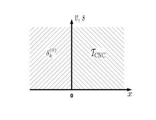
Figure 1: Numerical algorithms used for the Lerch transcendent.

Table 4: Acceleration of the convergence of the Lerch transcendent $\Phi(x,s,v)$ defined in Eq. (155). Results are presented for the set of parameters $x=0.99$, $s=1.1$ and $v=0.1$. In the first row, we indicate the quantity $n$ which is the order of the partial sum or alternatively the order of the transformation. In the second row, the partial sums $s_{n}=\sum_{k=0}^{n}x^{k}/(k+v)^{s}$ of the input series are given while in the third and the fourth rows we indicate the transformation $\delta^{(0)}_{n}(1,s_{0})$ and the CNCT transforms, respectively.

n	$s_{n}$	$\delta^{(0)}_{n}(1,s_{0})$	${\cal T}_{\rm CNC}(n)$
$1$	$\underline{1}3.480~{}716~{}950~{}334$	$\underline{1}4.323~{}956~{}240~{}313$	$\underline{16}.333~{}647~{}069~{}601$
$2$	$\underline{1}3.914~{}057~{}335~{}485$	$\underline{1}4.872~{}118~{}432~{}283$	$\underline{16.27}4~{}855~{}206~{}560$
$3$	$\underline{1}4.193~{}574~{}009~{}886$	$\underline{1}5.328~{}655~{}340~{}349$	$\underline{16.279~{}4}39~{}130~{}003$
$\dots$	$\dots$	$\dots$
$9$	$\underline{1}4.965~{}099~{}286~{}381$	$\underline{16}.183~{}960~{}654~{}046$	$\underline{16.279~{}415~{}474}~{}265$
$10$	$\underline{1}5.036~{}154~{}906~{}635$	$\underline{16.2}14~{}534~{}170~{}121$	$\underline{16.279~{}415~{}474}~{}379$
$11$	$\underline{1}5.099~{}561~{}126~{}734$	$\underline{16.2}35~{}397~{}170~{}154$	$\underline{16.279~{}415~{}474~{}45}7$
$12$	$\underline{1}5.156~{}650~{}914~{}411$	$\underline{16.2}49~{}604~{}756~{}607$	$\underline{16.279~{}415~{}474~{}45}7$
$13$	$\underline{1}5.208~{}442~{}487~{}775$	$\underline{16.2}59~{}256~{}744~{}711$	$\underline{16.279~{}415~{}474~{}453}$
$14$	$\underline{1}5.255~{}730~{}569~{}885$	$\underline{16.2}65~{}802~{}155~{}733$	$\underline{16.279~{}415~{}474~{}453}$
exact	$16.279~{}415~{}474~{}453$	$16.279~{}415~{}474~{}453$	$16.279~{}415~{}474~{}453$

Table 5: Same as Table 4 for $x=-0.99$, $s=1.1$ and $v=0.1$.

n	$s_{n}$	$\delta^{(0)}_{n}(1,s_{0})$	${\cal T}_{\rm CNC}(n)$
$1$	$\underline{11}.697~{}791~{}285~{}548$	$\underline{11.9}89~{}386~{}929~{}355$	$\underline{}9.312~{}621~{}614~{}169$
$2$	$\underline{1}2.131~{}131~{}670~{}698$	$\underline{11.96}5~{}797~{}543~{}541$	$\underline{}9.521~{}513~{}807~{}481$
$3$	$\underline{11}.851~{}614~{}996~{}297$	$\underline{11.967~{}0}38~{}897~{}324$	$\underline{}9.812~{}306~{}769~{}207$
$\dots$	$\dots$	$\dots$
$8$	$\underline{1}2.009~{}956~{}315~{}957$	$\underline{11.967~{}090~{}786~{}6}54$	$\underline{1}0.403~{}057~{}902~{}502$
$9$	$\underline{11.9}29~{}460~{}886~{}859$	$\underline{11.967~{}090~{}786~{}6}22$	$\underline{1}0.479~{}117~{}052~{}492$
$10$	$\underline{1}2.000~{}516~{}507~{}113$	$\underline{11.967~{}090~{}786~{}619}$	$\underline{1}0.547~{}006~{}982~{}924$
$11$	$\underline{11.9}37~{}110~{}287~{}014$	$\underline{11.967~{}090~{}786~{}619}$	$\underline{1}0.608~{}315~{}040~{}497$
exact	$11.967~{}090~{}786~{}619$	$11.967~{}090~{}786~{}619$	$11.967~{}090~{}786~{}619$

2.4 Applications of Sequence Transformations to Resummations

2.4.1 Simple Case: Incomplete Gamma Function

We follow the same strategy as in Sec. 2.3. As a simple example of a resummation algorithm (see Sec. 2.4.1), we discuss a possible implementation of the incomplete Gamma Function $\Gamma(0,x)$ for positive argument $x$, based on the resummation of the divergent large-$x$ asymptotic expansion, where the series is strictly alternating. Of course, the upshot will be in demonstrating that the resummation algorithm permits us to use the divergent large-$x$ asymptotic expansion also at small positive $x$ with good effect. A much more involved case, which demands an adaptive algorithm, is the fully relativistic hydrogen Green function, as discussed in Sec. 2.4.2.

We start our discussion on the application of nonlinear sequence transformations to the resummation of the divergent series from the computationof the incomplete Gamma function given by [161]

$$\Gamma(\alpha,z)\;=\;\int_{z}^{\infty}\;{\rm d}t\;e^{-t}\;t^{\alpha-1}\;.$$ (157)

For the sake of simplicity, below we restrict our analysis to the special case of $\alpha=0$ and of positive, real argument: $z\in\mathbbm{R}$, $z>0$. For such $z$, the incomplete Gamma function reads as

$$\Gamma(0,z)\;=\;\int_{z}^{\infty}\;{\rm d}t\;\frac{e^{-t}}{t}\;=\;-{\rm Ei}(-z)\;,$$ (158)

where ${\rm Ei}(z)$ is the standard exponential integral.

Usually, the evaluation the incomplete Gamma function (158) is traced back to the computation of its asymptotic expansion. The explicit form of such an expansion is however different for the cases of small and large arguments $z$. For example, while for large, positive $z$ the incomplete Gamma function $\Gamma(0,z)$ has the asymptotic expansion

$$\Gamma(0,z)\;=\;\frac{e^{-z}}{z}\;\sum_{n=0}^{\infty}\;(-1)^{n}\;n!\;\left(\frac{1}{z}\right)^{n}\,,\qquad z\to\infty\;,$$ (159)

a completely different series arises for $z\to 0$

$$\Gamma(0,z)\;=\;\ln z-\gamma+z-\frac{z^{2}}{4}+\frac{z^{3}}{18}+{\rm O}(z^{4})\,,\qquad z\to 0\;,$$ (160)

where $\gamma=0.577216\dots$ is Euler’s constant. It is clear that (160) has numerical advantages over (159) for small $z$, whereas for large $z$, one would certainly refrain from using (160).

As seen from Eqs. (159) and (160), asymptotic expansions can be utilized to compute the Gamma function $\Gamma(0,z)$ in the regions of the large ($z\to\infty$) and small ($z\to 0$) positive arguments $z$. The problem arises, however, for the intermediate values of $z$. In order to resum the divergent series for $z\to\infty$ and, hence, to compute the incomplete Gamma function for such (intermediate) $z$ region we may apply the $\delta$ transformation. That is, by using the partial sums of the alternating divergent series (159)

$$s_{n}\;=\;\frac{e^{-z}}{z}\;\sum_{k=0}^{n}\;(-1)^{k}\;k!\;\left(\frac{1}{z}\right)^{k}\,,$$ (161)

as input data for Eq. (101), it is possible to recover the actual value of the incomplete Gamma function to high accuracy, even at relatively small $z$. In Table 6, for example, the resummation of the asymptotic expansion (159), which is a priori valid only for large $z$, is performed for the case $z=1$. As seen from this Table, while the term–by–term summation of Eq. (159) fails to compute the Gamma function $\Gamma(0,z=1)$, the 26th-order transformation $\delta_{26}^{(n=0)}(1,s_{0})$ reproduces this values up to 16 decimal digits.

Table 6: Resummation of the large-$z$ asymptotic series for the function $\Gamma(0,z)=\exp(-z)/z\,\sum^{\infty}_{k=0}k!/(-z)^{k}$ at argument $z=1$ [see Eq. (159)]. In the first row, we indicate the quantity $n$ which is the order of the partial sum or alternatively the order of the transformation. In the second row, we list the partial sums $s_{n}=\exp(-z)/z\sum^{n}_{k=0}k!/(-z)^{k}$ [see Eq. (161)], whereas in the third row, the $\delta$ transforms are displayed. These are defined in (101).

$n$	$s_{n}$	$\delta^{(0)}_{n}(1,s_{0})$
$1$	$0.000~{}000~{}000~{}000~{}000\times 10^{0}$	$\underline{0.2}45~{}252~{}960~{}780~{}961$
$2$	$0.735~{}758~{}882~{}342~{}884\times 10^{0}$	$\underline{0.21}0~{}216~{}823~{}526~{}538$
$3$	$-1.471~{}517~{}764~{}685~{}769\times 10^{0}$	$\underline{0.2}20~{}040~{}039~{}579~{}180$
$4$	$7.357~{}588~{}823~{}428~{}846\times 10^{0}$	$\underline{}0.219~{}508~{}174~{}842~{}629$
$\dots$	$\dots$	$\dots$
$22$	$3.955~{}539~{}479~{}532~{}130\times 10^{20}$	$\underline{0.219~{}383~{}934~{}395~{}5}18$
$23$	$-9.114~{}871~{}523~{}102~{}565\times 10^{21}$	$\underline{0.219~{}383~{}934~{}395~{}5}19$
$24$	$2.191~{}353~{}397~{}822~{}361\times 10^{23}$	$\underline{0.219~{}383~{}934~{}395~{}520}$
$25$	$-5.487~{}119~{}942~{}851~{}230\times 10^{24}$	$\underline{0.219~{}383~{}934~{}395~{}520}$
$26$	$1.428~{}755~{}174~{}056~{}189\times 10^{26}$	$\underline{0.219~{}383~{}934~{}395~{}520}$
exact	$0.219~{}383~{}934~{}395~{}520$	$0.219~{}383~{}934~{}395~{}520$

2.4.2 Involved Case: Relativistic Hydrogen Green Function

In Sec. 2.4.1, we have demonstrated how nonlinear sequence transformations may be used for the resummation of the divergent series arising from the expansion of the incomplete Gamma function. Below another example for the application of the nonlinear sequence transformations will be discussed, which concerns the evaluation of the relativistic Green function. This function is known to be an essential ingredient in (relativistic) atomic physics and quantum mechanics, because it allows us to perform a summation over a complete spectrum of intermediate, virtual atomic states. Such a summation is required, for example, for describing quantum electrodynamic radiative corrections in atoms (see, e.g., Refs. [35, 162, 163, 164]), for the computation of hyperpolarizabilities and for the evaluation of two– (and multi–)photon processes (see, e.g., Ref. [165]).

The fully relativistic Green function of an electron bound in a hydrogenlike atom is given in terms of the Dirac Hamiltonian $H_{\rm D}=\vec{\alpha}\cdot\vec{p}+\beta\,m-Z\alpha/|\vec{x}|$, where the $\vec{\alpha}$ and $\beta$ are standard $4\times 4$-matrices [166] in the Dirac representation, $\vec{p}$ is the momentum operator, $Z$ is the nuclear charge number and $\alpha$ is the fine-structure constant. We use units in which $\hbar=c=\epsilon_{0}=1$ and write the Dirac–Coulomb Green function as

$$G(\vec{x}_{2},\vec{x}_{1},z)=\left<\vec{x}_{2}\left|\frac{1}{H_{\rm D}-z}\right|\vec{x}_{1}\right>\,.$$ (162)

Here, $z$ is an energy argument which is assumed to be manifestly complex rather than real values in some calculations. A closed-form representation of $G(\vec{x}_{2},\vec{x}_{1},z)$ is not known. However, it is possible and convenient to separate radial and angular variables, and to write the Green function in the following $4\times 4$-matrix representation [166, 167] for the fully relativistic calculations,

$$G(\vec{x}_{2},\vec{x}_{1},z)=\sum\limits_{\kappa\mu}\left(\begin{array}[]{cc}G^{11}_{\kappa}(x_{2},x_{1},z)\,\,\chi_{\kappa}^{\mu}(\hat{x}_{1})\,\chi_{\kappa}^{\mu{\dagger}}(\hat{x}_{2})&-{\rm i}\,G^{12}_{\kappa}(x_{2},x_{1},z)\,\,\chi_{\kappa}^{\mu}(\hat{x}_{1})\,\chi_{-\kappa}^{\mu{\dagger}}(\hat{x}_{2})\\[8.61108pt] {\rm i}\,G^{21}_{\kappa}(x_{2},x_{1},z)\,\,\chi_{-\kappa}^{\mu}(\hat{x}_{1})\,\chi_{\kappa}^{\mu{\dagger}}(\hat{x}_{2})&G^{22}_{\kappa}(x_{2},x_{1},z)\,\,\chi_{-\kappa}^{\mu}(\hat{x}_{1})\,\chi_{-\kappa}^{\mu{\dagger}}(\hat{x}_{2})\end{array}\right)\,.$$ (163)

Here, the radial variables are $x_{i}=|\vec{x}_{i}|$, and the unit vectors are $\hat{x}_{i}=\vec{x}_{i}/|\vec{x}_{i}|$. The symbol $\chi_{\kappa}^{\mu}(\hat{x})$ denotes the standard two-component Dirac spinor, as given e.g. in Refs. [168, 169],

$$\chi_{\kappa}^{\mu}(\hat{x})= \sum_{m}C^{j\mu}_{l\mu-m\,\frac{1}{2}m}Y_{l\mu-m}(\hat{x})\,\chi_{m}\,,\quad\chi_{\frac{1}{2}}=\left(\begin{array}[]{c}1\\ 0\end{array}\right)\,,\quad\chi_{-\frac{1}{2}}=\left(\begin{array}[]{c}0\\ 1\end{array}\right)\,,$$ (168)

$$l= \left|\kappa+\frac{1}{2}\right|-\frac{1}{2}\,,\quad j=|\kappa|-\frac{1}{2}\,,\quad\kappa=(-1)^{j+l+1/2}\,\left(j+\frac{1}{2}\right)\,,\quad$$ (169)

and the $C^{j\mu}_{l\mu-m\,\frac{1}{2}m}$ are Clebsch–Gordan coefficients in the conventions of Ref. [169]. In Eq. (163), the expressions of the form $\chi_{\kappa}^{\mu}(\hat{x}_{1})\,\chi_{\kappa}^{\mu{\dagger}}(\hat{x}_{2})$ are to be understood as dyadic products, i.e. as defining $2\times 2$ matrices. Of course, $\kappa$ has the meaning of a Dirac angular quantum number. The quantities $l$ and $j$ are the orbital and the total angular momentum quantum numbers, respectively, The components of the radial Green function are given in terms of the four quantities $G^{ab}_{\kappa}(x_{1},x_{2},z)$ with $a,b=1,2$, and these functions have been historically problematic as far as their numerical evaluation is concerned.

Indeed, as seen from Eq. (163), the evaluation of matrix elements involving the relativistic hydrogen Green function entails both angular and radial parts. In many cases, the angular part of the Green function can be evaluated using standard, yet sometimes cumbersome angular momentum algebra, while the computation of the radial functions $G^{ab}_{\kappa}(x_{2},x_{1},z)$ is known to be a very involved task. An explicit representation of these four components is given by [see, e.g., Eq. (A.16) in [170] and Eqs. (101), (108) and (109) in [171]]:

$$G^{11}_{\kappa}(x_{2},x_{1},z) = Q\,(1+z)\,A_{-}(\lambda,\nu,2cx_{2})\,B_{+}(\lambda,\nu,2cx_{1})\,,$$ (170a)

$$G^{12}_{\kappa}(x_{2},x_{1},z) = Q\,c\,A_{-}(\lambda,\nu,2cx_{2})\,B_{-}(\lambda,\nu,2cx_{2})\,,$$ (170b)

$$G^{21}_{\kappa}(x_{2},x_{1},z) = Q\,c\,A_{+}(\lambda,\nu,2cx_{2})\,B_{+}(\lambda,\nu,2cx_{2})\,,$$ (170c)

$$G^{22}_{\kappa}(x_{2},x_{1},z) = Q\,(1-z)\,A_{+}(\lambda,\nu,2cx_{2})\,B_{-}(\lambda,\nu,2cx_{2})\,.$$ (170d)

Here, the overall prefactor is

$$Q=\frac{1}{4\,c^{2}\,x_{2}\,x_{1}\,\sqrt{x_{2}\,x_{1}}}\,\frac{\Gamma(\lambda-\nu)}{\Gamma(1+2\,\lambda)}\,.$$ (171)

The quantity $c$ is given in terms of the (complex) energy variable $z$ as $c=\sqrt{1-z^{2}}$, and up to order $(Z\alpha)^{2}$, the quantity $\lambda$ is equivalent to the modulus of the Dirac angular momentum quantum number $\kappa$ ,

$$\lambda=\sqrt{\kappa^{2}-(Z\alpha)^{2}}=|\kappa|+{\rm O}(Z\alpha)^{2}\,.$$ (172)

Indeed, it is possible and sometimes even necessary to separate $\lambda$ into an integer part and a fractional remainder,

$$\lambda=|\kappa|-\zeta\,,\qquad\zeta=\frac{(Z\alpha)^{2}}{|\kappa|+\lambda}\,.$$ (173)

We here identify $\zeta$ as the fractional part of $\lambda$. Finally, $\nu$ is given in terms of the energy variable $z$ as

$$\nu=\frac{z}{\sqrt{1-z^{2}}}\,(Z\alpha)\,.$$ (174)

The quantities $A$ and $B$ in Eq. (170) are related to the two solutions, integrable at infinity and at the origin, respectively, of the corresponding radial Dirac equation, and given in terms of Whittaker $M$ and $W$ functions. The specific form is as follows:

$$A_{\pm}(\lambda,\nu,y) = \left(\lambda-\nu\right)\,M_{\nu-1/2,\lambda}(y)\pm\left(\kappa-\frac{Z\alpha}{\sqrt{1-z^{2}}}\right)\,M_{\nu+1/2,\lambda}(y)\,,$$ (175a)

$$B_{\pm}(\lambda,\nu,y) = \left(\kappa+\frac{Z\alpha}{\sqrt{1-z^{2}}}\right)\,W_{\nu-1/2,\lambda}(y)\pm W_{\nu+1/2,\lambda}(y)\,.$$ (175b)

As seen from Eq. (170), the computation of the radial Green functions can be traced back to the evaluation of the special Whittaker functions

$$M_{\nu\pm 1/2,\lambda}(y)\,,\qquad W_{\nu\pm 1/2,\lambda}(y)\,.$$ (176)

For purely real and purely imaginary values of the energy variable $z$, the quantity $c$ and thus the argument of the Whittaker functions remains purely real rather than complex. This situation is realized along special integration contours for the complex photon energy [170, 172, 35, 163, 164], but not universally applicable. We will assume here that in many practical applications, the complex argument of $y$ can be made small by choosing a suitable integration contour for the photon energy.

Here, we thus concentrate on numerical methods, some of which are based on nonlinear sequence transformations, which permit the evaluation of the $W_{\alpha_{\pm},\lambda}(x)$ and $M_{\alpha_{\pm},\lambda}(x)$ functions over a wide parameter range relevant for self-energy type calculation [170, 172, 35, 163, 164]. This parameter range can be characterized by the first parameter $\nu\pm 1/2$ being complex, but small in absolute magnitude, and the second parameter $\lambda$ being real, but possibly large in absolute magnitude. Pathological cases in which the parameters are close to integers, also have to be treated.

We rewrite the Whittaker functions $W$ and $M$ in terms of more fundamental hypergeometric $U$ and ${}_{1}F_{1}$ functions The $M$ functions occurring in (176) can be written as (see [173], p. 337 and [174], p. 296)

$$M_{\nu\pm 1/2,\lambda}(y) = e^{-\frac{1}{2}\,y}\,y^{\lambda+\frac{1}{2}}\,{{}_{1}}F_{1}\left(\frac{1}{2}\mp\frac{1}{2}+\lambda-\nu,2\,\lambda+1,y\right)$$ (177)

$$= e^{-\frac{1}{2}\,y}\,y^{|\kappa|+\frac{1}{2}-\zeta}\,\,{{}_{1}}F_{1}\left(|\kappa|+1-\delta_{\pm}-\zeta-\nu,2\,|\kappa|+1-2\,\zeta,y\right)\,,$$

whereas the $W$ functions can be rewritten in terms of the hypergeometric functions $U$ (see [175], p. 14)

$$W_{\nu\pm 1/2,\lambda}(y) = e^{-\frac{1}{2}\,y}\,y^{\lambda+\frac{1}{2}}\,\,U\left(\frac{1}{2}\mp\frac{1}{2}+\lambda-\nu,2\,\lambda+1,y\right)$$ (178)

$$= e^{-\frac{1}{2}\,y}\,y^{|\kappa|+\frac{1}{2}-\zeta}\,U\left(|\kappa|+1-\delta_{\pm}-\zeta-\nu,2\,|\kappa|+1-2\,\zeta,y\right)\,.$$

We here define the variable $\delta_{\pm}$ as

$$\delta_{\pm}=\left\{\begin{array}[]{cc}1&\mbox{for the case $+$\,,}\\[8.61108pt] 0&\mbox{for the case $-$\,.}\end{array}\right.$$ (179)

The transformations (177) and (178) generate ${}_{1}F_{1}$ and $U$ functions, which are given by

$${}_{1}F_{1}(a_{\pm},b_{\lambda},y)\qquad\mbox{and}\qquad U(a_{\pm},b_{\lambda},y)\,.$$ (180)

The parameters are

$$a_{\pm}=|\kappa|+1-\delta_{\pm}-\zeta-\nu\,,\qquad b_{\lambda}=2\,|\kappa|+1-2\,\zeta\,.$$ (181)

For the $W$ function, it is possible to rewrite the $U$ function as a ${}_{2}F_{0}$ (see [173], p. 342, [174], p. 317 and [175], p. 61)

$$W_{\nu\pm 1/2,\lambda}(y) = e^{-\frac{1}{2}\,y}\,y^{\nu\pm 1/2}\,{}_{2}F_{0}\left(\frac{1}{2}\mp\frac{1}{2}+\lambda-\nu,\frac{1}{2}\mp\frac{1}{2}-\lambda-\nu,-\frac{1}{y}\right)$$ (182)

$$= e^{-\frac{1}{2}\,y}\,y^{\nu\pm 1/2}\,{}_{2}F_{0}\left(|\kappa|+1-\delta_{\pm}-\zeta-\nu,-|\kappa|+1-\delta_{\pm}+\zeta-\nu,-\frac{1}{y}\right)$$

$$\sim e^{-\frac{1}{2}\,y}\,y^{\nu\pm 1/2}\,\sum_{k=0}^{\infty}\frac{\left(|\kappa|+1-\delta_{\pm}-\zeta-\nu\right)_{k}\,\left(-|\kappa|+1-\delta_{\pm}+\zeta-\nu\right)_{k}}{k!\,(-y)^{k}}\,.$$

This representation entails the Pochhammer symbol $(a)_{k}=\Gamma(a+k)/\Gamma(a)$ and constitutes the fundamental divergent asymptotic series of the $W$ function for large arguments (i.e., in inverse powers of $y$). Note, however, that because of the factorial growth of the numerators with $k$, the series eventually diverges no matter how large $y$ is. Nevertheless, we anticipate here that it can be used as an input for the resummation algorithms introduced in Chap. 2.2.3. We summarize that the transformation (182) has given rise to a ${}_{2}F_{0}$ function of arguments $a^{\prime}_{\pm}$ and $b^{\prime}_{\pm}$, where

$${}_{2}F_{0}(a^{\prime}_{\pm},b^{\prime}_{\pm},y)\,,\qquad a^{\prime}_{\pm}=a_{\pm}\,,\qquad b^{\prime}_{\pm}=-|\kappa|+1-\delta_{\pm}+\zeta-\nu\,.$$ (183)

The parameter $b^{\prime}_{\pm}$ can assume values very close to negative integers, if the absolute magnitude of $\nu$ and $\zeta$ is small. This entails a tremendous loss of numerical significance in high-precision calculations, if the asymptotic form of the ${}_{2}F_{0}$ function (182) is used for large $|\kappa|$ (the problematic terms originate for a summation index $k=|\kappa|-1+\delta_{\pm}$). In the numerical code, it is therefore crucial to separate all parameters of the hypergeometric functions into integer and fractional contributions.

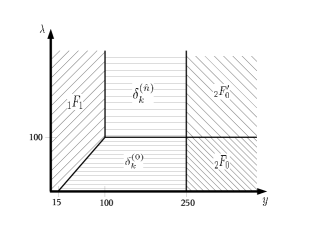
Figure 2: Numerical evaluation of the $W$ function.

A last representation useful for small $y$ is the decomposition of the $W$ function in terms of two ${}_{1}F_{1}$ functions,

$$W_{\nu\pm 1/2,\lambda}(y)=e^{-\frac{1}{2}\,y}\,y^{\lambda+\frac{1}{2}}\,\left[\frac{\Gamma(-2\,\lambda)}{\Gamma\left(\frac{1}{2}\mp\frac{1}{2}-\lambda-\nu\right)}\,{}_{1}F_{1}\left(\frac{1}{2}\mp\frac{1}{2}+\lambda-\nu,2\,\lambda+1,y\right)\right.$$ (184)

$$\;\;\;+\left.\frac{\Gamma(2\,\lambda)}{\Gamma\left(\frac{1}{2}\mp\frac{1}{2}+\lambda-\nu\right)}\,{}_{1}F_{1}\left(\frac{1}{2}\mp\frac{1}{2}-\lambda-\nu,1-2\,\lambda,y\right)\right]\,$$

$$=e^{-\frac{1}{2}\,y}\,y^{|\kappa|+\frac{1}{2}-\zeta}\,\left[\frac{\Gamma(-2\,|\kappa|+2\,\zeta)}{\Gamma\left(-|\kappa|+1-\delta_{\pm}-\nu+\zeta\right)}\,{}_{1}F_{1}\left(|\kappa|+1-\delta_{\pm}-\nu-\zeta,2\,|\kappa|+1-2\,\zeta,y\right)\right.$$

$$\;\;\;+\left.\frac{\Gamma(2\,|\kappa|-2\,\zeta)}{\Gamma\left(|\kappa|+1-\delta_{\pm}-\nu-\zeta\right)}\,{}_{1}F_{1}\left(-|\kappa|+1-\delta_{\pm}-\nu+\zeta,-2\,|\kappa|+1+2\,\zeta,x\right)\right]\,.$$

One of the two ${}_{1}F_{1}$ functions in Eq. (184) has parameters $a_{\pm}$ and $b_{\pm}$, and the other is of the form

$${}_{1}F_{1}(a^{\prime\prime}_{\pm},b^{\prime\prime}_{\pm},y)\,,\qquad a^{\prime\prime}_{\pm}=-|\kappa|+1-\delta_{\pm}-\nu+\zeta\,,\qquad b^{\prime\prime}_{\pm}=-2\,|\kappa|+1+2\,\zeta\,.$$ (185)

Again, numerical stability problems can result (both parameters $a^{\prime\prime}_{\pm}$ and $b^{\prime\prime}_{\pm}$ can be close to negative integers), and these can also be solved by a separation of the arguments into integer and fractional contributions.

We have thus mapped the problem of the calculation of the radial Dirac–Coulomb wave functions given in Eq. (163) onto the problem of evaluating the $M$ and $W$ functions listed in (176), or of evaluating the ${}_{1}F_{1}$ and $U$ function given in (180), (183) and (185), which is equivalent. The parameter range for $\nu$ required for the calculations reported in Refs. [35, 162, 163, 164] is approximately given by $\nu\in(0,n)$ for the so-called low-energy part (soft virtual photons and by $\nu\in{\rm i}\,(0,Z\alpha)$ for the high-energy part (hard virtual photons). The parameter range for $\nu$ thus is tiny in comparison to the parameter ranges for $\lambda$ and $y$, which both comprise the interval $(0,10^{7})$ in the high-precision calculations described in Refs. [35, 162, 163, 164].

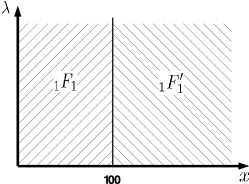
Figure 3: Numerical evaluation of the $M$ function.

For the $M$ and $W$ functions listed in Eq. (163), we can thus devise a numerical algorithm which in each case depends only on the value of the second parameter $\lambda$ and of the argument $y$, not on the value of the first parameter $\nu$. For the $W$ function, a rather sophisticated differentiated treatment of the different parameters is required. All the choices are summarized in Fig. 2. The explanation is a follows:

• Algorithm labeled “${}_{1}F_{1}$”: We decompose the $W$ function into two hypergeometric ${}_{1}F_{1}$ functions as in Eq. (184). The two ${}_{1}F_{1}$ functions are evaluated by virtue of their defining power series (in the argument $y$). Suitable truncation criteria for the power series can be constructed according to Eqs. (D.3) and D.10) of Ref. [172] for the first and the second ${}_{1}F_{1}$ function on the right-hand side of Eq. (184).

• Algorithms labeled “$\delta^{(0)}_{k}$” and “$\delta^{(\hat{n})}_{k}$”: In an intermediate range of arguments $\lambda$ for the $W$ function, we use the divergent asymptotic series on the right-hand side of Eq. (182) as input for the sequence transformation (101).

  $$s_{n}=\sum_{k=0}^{n}\frac{\left(|\kappa|+1-\delta_{\pm}-\zeta-\nu\right)_{k}\,\left(-|\kappa|+1-\delta_{\pm}+\zeta-\nu\right)_{k}}{k!\,(-y)^{k}}\,.$$ (186)

  The asymptotic series is resummed either via the nonlinear sequence transformation

  $${\delta}_{k}^{(0)}(1,s_{0})\qquad\mbox{(algorithm ``$\delta^{(0)}_{k}$'')}$$ (187)

  or

  $${\delta}_{k}^{(\hat{n})}(1,s_{\hat{n}})\qquad\mbox{(algorithm ``$\delta^{(\hat{n})}_{k}$'')}$$ (188)

  where

  $$\hat{n}=[\mkern-2.5mu[{\rm Re}(|\kappa|-1+\delta_{\pm}-\zeta+\nu)]\mkern-2.5mu]\,.$$ (189)

  Note that in this notation, $k$ refers to the order of the transformation, which is subsequently increased until convergence is reached. By contrast, $\hat{n}$ refers to the element in the asymptotic series beyond which the transformation is started, according to the definition in Eq. (101). The resummation of the asymptotic series yields values for the $W$ function accurate to at least a relative precision of at least $10^{-24}$, in the parameter regions indicated in Fig. 2.

• Algorithms “${}_{2}F_{0}$” and “${}_{2}F^{\prime}_{0}$”: For large $y$, the asymptotic series (182) of the ${}_{2}F_{0}$ function is suitably truncated, according to criteria found in the Eqs. (D.6), (E.14) and (E.15) of Ref. [172]. For “${}_{2}F_{0}$”, the asymptotic series is summed from the first element $k=1$ in Eq. (182). For cases where both $\lambda$ and $x$ are large, the asymptotic series is summed in both upward and downward directions from the element of maximum absolute magnitude in both directions (algorithm “${}_{2}F^{\prime}_{0}$”).

The first decisive observation in the context of the current review is that the nonlinear sequence transformation (101) can be used in order to bridge an intermediate region where a suitable truncation of the asymptotic series (182) fails to produce results of sufficient accuracy, because the argument $y$ is not sufficiently large, and yet the power series representation of the $W$ function in terms of two ${}_{1}F_{1}$’s according to (184) also fails because of numerical losses due to cancellations among the two confluent hypergeometric functions. The second decisive observation, in the context of the current review is that a simple, brute-force implementation of this idea cannot succeed, and that considerable further sophistication is required if large parameter ranges are to be covered. In particular, the separation into the “$\delta^{(0)}_{k}$” and “$\delta^{(\hat{n})}_{k}$” algorithms, counterintuitive at first glance, constitutes one of the keys to a numerically effective evaluation of the Dirac–Coulomb Green function (163).

For the $M$ function in Eq. (176), we use an evaluation scheme illustrated in Fig. 3. For small arguments, the $M$ function is evaluated by summing the power series of the ${}_{1}F_{1}$ function in Eq. (177), starting with the first element of this power series. This region is denoted as “${}_{1}F_{1}$” in Fig. 2. The elements of the power series of the confluent hypergeometric function are evaluated recursively in analogy to Eq. (D.5) in [172], and a termination criterion analogous to (D.6) in [172] is used. For large arguments, the power series is also used, but summation is started with the element of the power series with the largest absolute magnitude. This maximum element is determined as outlined in Appendix E of [172], and summation in the upward and downward direction is terminated by criteria analogous to (E.9) and (E.10) in [172]. The relevant region is denoted as “${}_{1}F^{\prime}_{1}$” in Fig. 2.

In the current application just shown we have discussed the accelerated pointwise evaluation of special functions by applying convergence acceleration and summation processes to their defining expansions. In the same light, it should be stressed that quite recently [36], the same strategy has been proposed for the pointwise evaluation of Fourier series and other expansions (e.g., those into orthogonal polynomials). Namely, it has been observed that the application of the simple $\epsilon$ algorithm to Fourier series of functions with discontinuities leads to an acceleration of the convergence of the Fourier series, and that the Gibbs “overshooting” phenomenon can be significantly reduced. A slight generalization of the problem using complex variables turns out to be beneficial in the latter context. One defines the Fourier conjugate series ${\tilde{S}}(t)$ of a Fourier series $S(t)$ with a zero constant term by the following relations,

$$S(t)= \;\sum_{k=1}^{\infty}a_{k}\,\cos(k\,t)+\sum_{k=1}^{\infty}b_{k}\,\sin(k\,t)\,,$$ (190)

$${\tilde{S}}(t)= \;\sum_{k=1}^{\infty}a_{k}\,\sin(k\,t)-\sum_{k=1}^{\infty}b_{k}\,\cos(k\,t)\,,$$ (191)

$$F(t)= \;S(t)+{\rm i}\,{\tilde{S}}(t)\;=\;\sum_{k=1}^{\infty}(a_{k}-{\rm i}\,b_{k})\,\exp({\rm i}\,k\,t)\,.$$ (192)

In many cases [36], the series $S(t)={\rm Re}\,F(t)$ can be numerically determined to good accuracy by applying the $\epsilon$ algorithm to the complex series $F(t)$, and selecting the real part of the calculated complex Padé approximants to $F(t)$. Note that the calculations described here for the relativistic hydrogen Green function also necessitate the application of convergence accelerators “in the complex plane,” as the energy variable $z$ and, consequently, the parameter $\lambda$ defined in Eq. (172) can assume complex values. With these remarks, we would like to close the discussion of the convergence accelerators and turn our attention to the summation of divergent series.

3 Borel Summation

The contents of the current section on Borel summation can be summarized as follows.

• In Sec. 3.1, a crude guidance for the reader is provided, and some basic properties of the Borel summation process are reviewed.

• In Sec. 3.3, the performance of a number of resummation algorithms is studied using zero-dimensional model theories as example.

• In Secs. 3.4, 3.5 and 3.6, we discuss both the mathematical theorems governing the large-order behaviour of the perturbation theory of anharmonic oscillators, as well as the practical summation of the perturbative expansions, in a number of cases of special interest.

• In Sec. 3.7, some connections of both summation processes as well as convergence accelerators to the renormalization group, and to the determination of critical exponents, is discussed.

3.1 Quick Start

Why should there be another review article on Borel summation in quantum mechanics and field theory? This question may well be asked in view of a number of excellent review articles on related subjects. Here is an incomplete list: The development of large-order perturbation theory with a special emphasis on the determination of critical exponents of second-order phase transitions has been authoritatively summarized in Refs. [176, 177]. The development of generalized perturbative expansions with applications to quantum mechanical problems has been described in Ref. [178], and further works [179, 180, 181]. The generalized perturbative expansions, which are also known as resurgent expansions, and their connection to perturbation series in quantum chromodynamics has been explored in other works (e.g., Refs. [182, 183, 184, 185, 186, 187]). The so-called Lipatov asymptotic form, which describes factorially divergent contributions to perturbation series due to the explosion of the number of Feynman diagrams in higher orders, has been discussed in Ref. [69]. Finally, the significance of so-called renormalons has been elucidated in Ref. [188]: these are additional factorially divergent contributions to perturbation series due to a specific type of diagrams whose number does not explode in higher orders (but whose numerical coefficients do).

The answer to the provocative question which was asked in the beginning of the last paragraph is as follows: We are trying here to accomplish three goals:

1. Our first goal is to establish a connection between the physics literature on the subject, and several interesting theorems which have been proven on the mathematical side of the field, and to illustrate the concept of distributional Borel summability [189, 190] by a number of concrete calculations and mathematical considerations.

2. Our second goal is to describe the current status, and possible further developments, of the field in the direction of an enhanced perturbative calculation of critical exponents, where a lot of effort has already been placed and where progress eventually relies on a combined effort along a careful technical analysis of the problem of parameterizing Feynman amplitudes, on the sophisticated use of modern high-performance computers, and on numerical algorithms.

3. Our third goal is to illustrate various connections of the divergent series to physical processes, and to illustrate that a number of phenomena would be less well understood today were it not for the fruitful combination of results from mathematics and physics in a field which has matured only recently.

In Appendix C, we discuss very briefly how the concept of a resurgent expansion [64], which has already proven to be very useful in quantum mechanics, could be useful to justify certain remainder estimates for divergent perturbation series in quantum chromodynamics. Many of the sophistications discussed here can be summarized under the unifying concept of the singularities of the Borel transform in the “Borel plane” spanned by the argument of the Borel transform.

Observe that the singularities in the Borel plane have got nothing to do with the so-called Bender–Wu cuts which are encountered when the coupling constant of anharmonic problems is continued analytically into the complex plane [55, 56, 57]. Namely, it has been shown that the energy levels of typical anharmonic oscillators (e.g., with a $g\,x^{4}$ perturbation) behave as multi-valued functions when the coupling constant $g$ is continued analytically into the complex plane: They have branch cuts. For the quartic perturbation, the branch points and cuts are known (see Ref. [55]) to occur near ${\rm arg}\,g\approx\pi/2$ and ${\rm arg}\,g\approx 3\pi/2$. The branch cuts are “short” in the sense that they only extend to angles of a few degrees about the quoted complex arguments of $g$. For a detailed discussion, we refer to Refs. [55, 56, 57], but a short detour is in order.

Let us suppose that we start with a particular real $g$ and follow a particular energy eigenvalue $E\equiv E(g)$ as a function of complex $g$, as $g$ is varied along a path in the complex plane and crosses a Bender–Wu branch cut, and let us suppose that $g$ is again varied on the other Riemann sheet toward the real axis and to the starting value of $g$: we end up with a different eigenvalue $E(g)$. In some sense, the Bender–Wu branch cuts offer “loopholes” in the complex plane that join the energy eigenvalues of the problem. Another curious observation is as follows: suppose we vary $g$ scraping a branch cut, directly and exactly through a branch point, perpendicular to the scraped branch cut. Let us suppose, furthermore, that we follow the evolution of the functions $E_{{\rm I}\to{\rm II}}(g)$ and $E_{{\rm II}\to{\rm I}}(g)$ that correspond to crossing from branch cut from sheet I to sheet II and vice versa, across the branch point: the surprising conclusion [55] is that the two functions $E_{{\rm I}\to{\rm II}}(g)$ and $E_{{\rm II}\to{\rm I}}(g)$ will cross at the branch point, and this constitutes a level crossing as a function of $g$. These and related observations have been crucial for the development of the mathematical theory of the anharmonic oscillators and related problems, which is summarized here in the form of a number of theorems. In a further context, the investigation of complex coupling constants has inspired the development of dilation analyticity [191] (sometimes called “dilatation” analyticity) which has proven to be a crucial tool for the calculation of complex resonance energies which include an imaginary part (a decay width). Yet, the analytic continuation of $g$ into the complex plane does not always provide additional insight in the case of the practical problem of obtaining optimized resummed values of perturbation series for a given, real, concrete value of $g$, based on a finite number of known coefficients. Problems of that sort are also investigated in this review.

In Sec. 2.1, we have given a collection of “recipes” as a guide to the selection of the convergence acceleration methods. An analogy of the “recipe” collection for the resummation of divergent series is much more difficult to provide, and we will resist the temptation to give one here. The reason is that while the discussion in Sec. 2 covers a number of algorithms, we here focus on only one: the Borel summation. We trust that the numerous examples treated here will serve as an intuitive guidance for the interested reader, when a new problem is encountered.

3.2 Selected Methods

3.2.1 General Formulas

Since its introduction [45, 46], the Borel method has been found to be a very powerful and elegant tool in quantum mechanics as well as in quantum field theory and, therefore, has been discussed in details in an enormous literature (see, e.g., pp. 233—238 of [192], pp. 453—456 of [193], pp. 880—887 of [177], pp. 465—466 of [194], pp. 373—376 of [195], pp. 87—92 of [196], pp. 54—56 of [197], and pp. 743—744 of [198], as well as the seminal work [199]). Let us start our discussion with the asymptotic, divergent perturbative expansion of some physical observable $f(g)$ in powers of a coupling parameter $g$. We exchange the argument $z$ of the function defined in Eq. (22) by $g$ and redefine the perturbative coefficients according to $\alpha_{n}\to a_{n}$, as is customary in the literature,

$$f(g)\sim\sum\limits_{n=0}^{\infty}a_{n}\,g^{n}\,,\qquad g\to 0\,.$$ (193)

Moreover, we assume that the coefficients $a_{n}$ of this series grow factorially as $n\to\infty$, and that $f(g)$ is analytic in a suitable sectorial region of the complex $g$-plane. Then the Borel transformed series

$$B_{f}(u)\;=\;\sum_{n=0}^{\infty}\,\frac{a_{n}}{n!}\,u^{n}\;=\;\sum_{n=0}^{\infty}\,\frac{a_{n}}{\Gamma(n+1)}\,u^{n}$$ (194)

converges in some circle around $u=0$ by the Cauchy–Hadamard theorem because by assumption $|a_{n}|/n!<A^{n}$ for some $A>0$. That is, the series (194) possesses a nonzero radius of convergence $\rho>0$, and $B_{f}(u)$ is analytic in the circle of radius $\rho$ centered at $u=0$.

We can now make use of the relationship $n!\,=\,\int_{0}^{\infty}u^{n}{\rm e}^{-u}{\rm d}u$, interchange summation and integration so that $f(g)$ can be represented by the following Laplace integral (see for example Theorem 122 on p. 182 of [6] or p. 141 of [173]),

$$f(g)\;=\;\frac{1}{g}\,\int_{0}^{\infty}\,\exp(-u/g)\,B_{f}(u)\,{\rm d}u\,.$$ (195)

The case that the series (194) for $B_{f}(u)$ converges for all $u\in[0,\infty)$ actually cannot occur here since we explicitly assumed above that the coefficients $a_{n}$ of the formal power series (22) for $f(g)$ grow factorially as $n\to\infty$. The representation of $f(g)$ by the Laplace integral (195) is valid provided that $B_{f}(u)$ admits an analytic continuation to a neighborhood of the positive real semiaxis such that $B_{f}(u)$ grows at most exponentially as $u\to\infty$ (see for example p. 141 of [173]), so that the Laplace–Borel (195) integral converges at the upper limit. Then, the Laplace integral (195) exists for some $g>0$ and provides a finite expression for $f(g)$ even if the perturbation series (22) diverges for every $g\neq 0$.

The Borel summation process can be easily generalized. Let us now assume that a physical quantity $F(g)$ admits an asymptotic expansion,

$$F(g)\sim\sum\limits_{n=0}^{\infty}a_{n}\,g^{n}\,,\qquad g\to 0\,,\qquad|a_{n}|\;\leq\;C\,\sigma^{n}\,\Gamma(kn+1)\,,$$ (196)

for some rational number $k\geq 1$ and for all integer $n$ with $C$ and $\sigma$ as suitable positive constants. Then we define the Borel transform of order $k$ as

$$B^{(k)}_{F}(u)\;=\;\sum_{n=0}^{\infty}\,\frac{a_{n}}{\Gamma(kn+1)}\,u^{n}\,.$$ (197)

By construction, this series converges in the circle of radius $\rho\equiv\sigma^{-1}$ around $u=0$. If $B^{(k)}_{F}(u)$ can be analytically continued from its circle of convergence to the whole positive real semiaxis, and the continuation is bounded by $e^{u^{1/k}}$ as $u\to+\infty$, then $F(g)$ can be expressed by the Laplace integral (see [200] or Example 3 on p. 45 and Problem 29(b) on p. 73 of [44])

$$F(g)\;=\;\frac{1}{kg}\,\int_{0}^{\infty}\,B^{(k)}_{F}(u)\,\exp\left[-\left(\frac{u}{g}\right)^{1/k}\right]\,\left(\frac{u}{g}\right)^{1/k-1}\,{\rm d}u\,.$$ (198)

Under certain conditions, the Borel summation process can even be generalized in such a way that perturbation expansions can be summed whose coefficients $a_{n}$ grow like $\Gamma(kn+1)\exp(\alpha n^{2}/4)$, with $k$ and $\alpha$ being suitable positive constants [201, 202].

Let us now consider two simple examples,

$${\cal A}(g)=\sum_{n=0}^{\infty}(-1)^{n}\,n!\,g^{n}$$ (199)

and

$${\cal N}(g)=\sum_{n=0}^{\infty}n!\,g^{n}\,.$$ (200)

The series ${\cal A}(g)$ actually constitutes the so-called Euler series (see Sec. 13.3 of Ref. [31]), which has often been used as a paradigmatic example of a factorially divergent, asymptotic series in the literature. The Borel transforms have a unit radius of convergence and read

$$B_{\cal A}(u)\;=\;\sum_{n=0}^{\infty}\,(-1)^{n}\,u^{n}\;=\;\frac{1}{1+u}\,,\qquad B_{\cal N}(u)\;=\;\frac{1}{1-u}\,.$$ (201)

By inserting the above formulas, which actually constitute analytic continuations for $u>1$, into the Laplace integral (195) we find the Borel sums

$${\cal A}(g)\;=\;\frac{1}{g}\,\int_{0}^{\infty}\,\frac{\exp(-u/g)\,{\rm d}u}{1+u}\,,\qquad{\cal N}(g)\;=\;\frac{1}{g}\,\int_{0}^{\infty}\,\frac{\exp(-u/g)\,{\rm d}u}{1-u}\,,$$ (202)

The Borel sum of ${\cal A}(g)$ is well defined and may be expressed as [see, e.g., Eq. (3.02) on p. 40 of [76]]

$${\cal A}(g)\;=\;\frac{1}{g}\,\exp(1/g)\,E_{1}(1/g)\,,$$ (203)

where

$$E_{1}(g)\;=\;\int_{g}^{\infty}\,t^{-1}\,{\rm e}^{-t}\,{\rm d}t\,,\qquad|\arg(g)|\leq\pi/2$$ (204)

is an exponential integral.

In the case of ${\cal N}(g)$, the analytic continuation (201) has a pole for $g=1$ so that the Laplace–Borel integral has a singularity for every $g>0$ on the integration path and does not define an analytic function of $g$. In view of these complications, it is not immediately obvious in what sense the integral representation (202) can be associated with ${\cal N}(g)$ and used for its evaluation. One may choose a principal-value prescription or encircle the pole in either the positive or the negative sense. Indeed, we have [see, e.g., Eq. (3.08) on p. 41 of [76]]:

$$E_{1}(-x\pm i0)\;=\;-{\rm Ei}(x)\mp{\rm i}\,\pi\,,\quad x>0\,,$$ (205)

where

$${\rm Ei}(x)\;=\;-{\rm PP}\,\int_{-\infty}^{x}\,t^{-1}\,{\rm e}^{t}\,{\rm d}t$$ (206)

is the exponential integral defined as a Cauchy principal value (principal part, $\mathrm{PP}$) for $x>0$. The notation $E_{1}(-x\pm i0)$ denotes the principal branch of $E_{1}(-x)$ on the upper $(+)$ and lower $(-)$ side of the cut along the negative real axis, respectively. Thus, ${\cal N}(g)$ defined by the divergent series (200) can for $g>0$ be expressed as follows:

$${\cal N}(g)\;=\;\frac{1}{g}\,\exp(-1/g)\,\left[{\rm Ei}(1/g)+\left\{\begin{array}[]{cc}0&\mbox{(principal value prescription)}\\ {\rm i}\,\pi&\mbox{(lower contour)}\\ -{\rm i}\,\pi&\mbox{(upper contour)}\end{array}\right.\right]\,.$$ (207)

We will later see that all these possibilities are actually realized in physically relevant examples. The sign of the imaginary part, if it exists, can mostly be fixed on the basis on an immediate consideration (e.g., a resonance energy eigenvalue has to describe a decaying, not an exponentially growing state as time increases). However, there are also situations, as already mentioned in Sec. 3.2.1, where the presence of a singularity along the integration path of the Laplace–Borel integral indicates the existence of additional contributions that cannot be obtained on the basis of perturbation theory alone.

3.2.2 Mathematical Foundations of Borel Summability

One of the purposes of this review is to form a bridge between mathematics and physics, by discussing exact available mathematical results regarding the Borel summability of specific perturbation series. We will thus need, in the current subsection, concepts recalled in Appendix A, in particular the notions of the resolvent, the spectrum and the Green function defined in Appendix A.1 and that of an analytic continuation of the resolvent to the second sheet of its Riemann surface, which defines a resonance and is described in Appendix A.2.

Let us also recall that for the convergent case, the concept of holomorphy establishes a one-to-one correspondence between convergent power series and functions of complex variables: this is the Weierstrass notion of analytic functions. If convergent power series are replaced by divergent ones, this one-to-one correspondence is in general impossible, because infinitely many functions of a complex variable singular at a point (without loss the origin) may admit the same divergent power series expansion. Consider the example ${\cal A}(g)$ given by (203). We know that its series expansion as $|g|\to 0$, $|{\rm arg}\,g|<\pi$ is $\sum_{n=0}^{\infty}n!\,(-g)^{n}$. However, any function ${\cal A}(g)+e^{-g^{-1/q}}$, with $q\geq 0$, admits the same divergent expansion as $|g|\to 0$ in the same directions. Additional requirements, such as uniform remainder estimates, are thus required to set up one-to-one correspondences between divergent power series and classes of analytic functions. In any physical problem giving rise to a divergent perturbation expansion, the most important thing to check in order to assign the correct meaning to the expansion is that this series and the solution fulfill the appropriate additional requirements.

The fundamental result in this connection is a classical theorem of Carleman [203]. Before we state the theorem, we need to recall some basic definitions and in particular, the fact that the condition ${\rm Re}\,g^{-1}>R^{-1}$ for a complex coupling constant $g$ defines the inner region of a circle of radius $R$ centered at ${\rm Re}\,g=R/2$, ${\rm Im}\,g=0$ in the complex $g$-plane.

Definition 1

Let $R>0$ and let $f(g)$ be a function analytic in the circle $C_{R}\equiv\{g\in{\mathbbm{C}}:{\rm Re}\,g^{-1}>R^{-1}\}$ of radius $R$. We say that a power series $\sum_{n=0}^{\infty}a_{n}\,g^{n}$ is asymptotic to $f$, or that $f$ admits a $\sum_{n=0}^{\infty}a_{n}\,g^{n}$ as an asymptotic expansion (to all orders) as $g\to 0$ in $C_{R}$ if, for each fixed $N$:

$$\left|f(g)-\sum_{n=0}^{N}a_{n}\,g^{n}\right|=O(g^{N+1}),\qquad g\to 0,\>\>g\in C_{R}\,.$$ (208)

It is easy to check that a function has at most one asymptotic expansion as $g\to 0$ in $C_{R}$. On the contrary, infinitely many functions may admit the same asymptotic expansion in a prescribed region. For example, if the function $f(g)$ satisfies Definition 1 above, then any function of the form $f(g)+A\,e^{-1/g}$, $A\in{\mathbbm{C}}$, admits as well $\sum_{n=0}^{\infty}a_{n}\,g^{n}$ as an asymptotic expansion as $g\to 0$ in $C_{R}$ because $A\,\exp(-1/g)$ has an identically zero asymptotic expansion therein. In order to establish a one-to-one correspondence between a function and a (possibly divergent) power series expansion a stronger condition than the one given in Definition 1 is needed, which is as follows.

Definition 2

Let $C_{R}$ be as above. We say that a function $f(g)$ analytic in $C_{R}$ obeys a strong asymptotic condition and admits $\sum_{n=0}^{\infty}a_{n}g^{n}$ as a strong asymptotic series in $C_{R}$ if there are $A,B>0$ such that

$$\left|f(g)-\sum_{n=0}^{N-1}a_{n}\,g^{n}\right|\leq A\,B^{N}\,N!\,|g|^{N}\,,\qquad\forall\;g\in C_{R}\,.$$ (209)

We can finally state Carleman’s theorem:

Theorem 3

(Carleman) If $\sum_{n=0}^{\infty}a_{n}\,g^{n}$ is a strong asymptotic series for two analytic functions $f$ and $g$, then $f\equiv g$. Moreover, there are $A$ and $B>0$ such that

$$|a_{n}|\leq A\,B^{n}\,n!\,,\qquad\forall\;n\in{\mathbbm{N}}_{0}\,.$$ (210)

Proof. See, e.g., Carleman’s book [203].

The following remarks are in order. Carleman proves also the necessity of the condition (209), in the sense that no weaker condition can guarantee the result. Functions admitting an asymptotic expansion with the above properties are thus determined by the series even if divergent and they are therefore called quasi-analytic. Observe that the convergence of a power series yields by definition a constructive approximation method for its sum. By the same definition, this cannot be extended to divergent series even when the conditions of Carleman’s theorem are satisfied.

Therefore the notion of a regular summation method is introduced: given a pair $(f(g),\sum_{n=0}^{\infty}a_{n}\,g^{n})$ fulfilling the conditions of Carleman’s theorem, a regular summation method is a constructive procedure which makes it possible to recover $f(g)$ out of the divergent power series and yields the ordinary sum when the series is convergent. In other words, when applicable, a summation method makes it possible to associate a unique analytic function to a given divergent series. In general the validity of a regular summation method requires much stronger conditions on $f(g)$ and $\sum_{n=0}^{\infty}a_{n}g^{n}$ than those of Carleman’s theorem. An example is the Stieltjes method, equivalent to the convergence of the Padé approximants, which requires very restrictive conditions both on $f$ and on $\sum_{n=0}^{\infty}a_{n}\,g^{n}$ as recalled below. A classical result of Nevanlinna [204], however (see also Sokal, Ref. [205]), singles out the Borel method as described above as the one which requires just the conditions of Carleman’s theorem. We have indeed

Theorem 4

(Nevanlinna) Under the conditions of Carleman’s theorem, the divergent series $\sum_{n=0}^{\infty}a_{n}\,g^{n}$ is Borel summable to $f(g)$ for $g$ real, $0\leq g<R$. This means the following: (i) The Borel transform $B_{f}(u)=\sum_{n=0}^{\infty}\frac{a_{n}}{n!}u^{n}$, a priori holomorphic within a circle of convergence of radius $B^{-1}$, i.e. for $|u|<B^{-1}$ where $B$ is given in Eq. (210), admits an analytic continuation to the strip $\{u\in{\mathbbm{C}}\,:\,|{\rm Im}\,{u}|<T\,,{\rm Re}\,u>0\}$. (ii) The Laplace integral $1/g\int_{0}^{\infty}B(u)\,{\rm e}^{-u/g}\,{\rm d}u$ converges absolutely for $0\leq g<T$ and for these values of $g$ one has

$$f(g)=\frac{1}{g}\,\int_{0}^{\infty}B_{f}(u)\,{\rm e}^{-u/g}\,{\rm d}u\,.$$ (211)

Proof. For a modern presentation, see [205].

In many instances, as we shall explicitly see later on in the examples from quantum physics, it is actually possible to verify a stronger statement for Borel summability, valid for functions $f(g)$ holomorphic in the sector $|{\rm arg}\,g|<\frac{\pi}{2}+\epsilon$ with $\epsilon>0$. Namely, we have the following theorem.

Theorem 5

(Watson-Nevanlinna) Let the pair $(f(g),\sum_{n=0}^{\infty}\frac{a_{n}}{n!}\,g^{n})$ fulfill the following conditions: (i) $f(g)$ is holomorphic in the open sector $\Omega_{\pi/2+\epsilon}\equiv\{g\in{\mathbbm{C}}\setminus\{0\}\,:\,|{\rm arg}\,g|<\frac{\pi}{2}+\epsilon\}$, with $\epsilon>0$, and continuous up to the boundary. (ii) $f(g)$ admits $\sum_{n=0}^{\infty}a_{n}\,g^{n}$ as a strong asymptotic expansion to all orders as $|g|\to 0$ in $\Omega_{\pi/2+\epsilon}$, i.e. there are $A>0$, $B>0$ such that, for $N\in\mathbb{N}$

$$\left|f(g)-\sum_{n=0}^{N-1}a_{n}\,g^{n}\right|\leq A\,B^{N}\,N!\,|g|^{N},\qquad|g|\to 0,\quad g\in\Omega_{\pi/2+\epsilon}$$ (212)

Then the series $\sum_{n=0}^{\infty}a_{n}g^{n}$ is Borel summable to $f(g)$ for all complex $g$ in the closure of the sector $\Omega^{B}_{\epsilon}\equiv\{g\in{\mathbbm{C}}:\,0<|g|<B^{-1}\;;|{\rm arg}\,g|<\epsilon\}$.

Proof. This classic result is proven for instance in the book of Hardy [6]. Another proof can be found in Ch. XII.3 of Ref. [44].

As before, all these results can be extended to series diverging as $n!^{\alpha}$ for any $\alpha>1$ provided the function $f(g)$ is analytic in a wider sector, the rule of thumb being: a sector of opening $\pi$ both in analyticity and in the validity of the remainder estimate is necessary to absorb any $n!$. Thus, an analyticity sector of opening at least $2\pi$ is necessary to absorb a divergence as $n!^{2}$, and so on. Obviously, the analyticity is intended on a Riemann surface sector when the opening angle exceeds $2\pi$. We limit ourselves to state the analogue of the Watson-Nevanlinna criterion for the Borel summability of order $k>1$, in the sense of Eq. (198), remembering that $k=1$ corresponding to ordinary Borel summability.

Theorem 6

(Nevanlinna-Leroy) Consider once again the pair $(f(g),\sum_{n=0}^{\infty}\frac{a_{n}}{n!}g^{n})$, this time under the following conditions: (i) For some rational number $k>0$, $f(g)$ is analytic in the circle $C_{R}\equiv\{g\in{\mathbbm{C}}:{\rm Re}\,g^{-1/k}>R^{-1}\}$. (ii) The function $f(g)$ admits $\sum_{n=0}^{\infty}a_{n}\,g^{n}$ as a strong asymptotic expansion to all orders as $|g|\to 0$ in $C_{R}$, i.e. there are $A>0$, $B>0$ so that, for $N\in{\mathbbm{N}}$ and $|g|\to 0,g\in C_{R}$:

$$\left|f(g)-\sum_{n=0}^{N-1}a_{n}\,g^{n}\right|\leq A\,B^{N}\,\Gamma(k\,N+1)\,|g|^{N}\,.$$ (213)

Then the series $\sum_{n=0}^{\infty}a_{n}\,g^{n}$ is Borel-Leroy summable of order $k$ to $f(g)$ for $g$ real, $0\leq g<R$. This means that the Borel-Leroy transform of order $k$,

$$B^{(k)}_{f}(u)=\sum_{n=0}^{\infty}\frac{a_{n}}{\Gamma(k\,n+1)}\,u^{n}\,,$$ (214)

a priori holomorphic for $|u|<B^{-1}$, admits an analytic continuation to the strip $\{u\in{\mathbbm{C}}\,:\,|{\rm Im}\,u|<R\,,\,{\rm Re}\,u>0\}$ and, for $0\leq u<R$, one has

$$f(g)=\frac{1}{k\,g}\,\int_{0}^{\infty}\,B^{(k)}_{f}(u)\,\exp\left[-\left(\frac{u}{g}\right)^{1/k}\right]\,\left(\frac{u}{g}\right)^{1/k-1}\,{\rm d}u\,,$$ (215)

where the integral in the right side converges absolutely.

As above, in many examples where the perturbation series diverges as fast as $(k\,n)!$ with $k>1$, it is actually possible to verify more, namely the validity of the generalized Watson-Nevanlinna criterion, where the analyticity requirement is extended from a disk $C_{R}$ to an open Riemann surface sector.

Theorem 7

(Watson-Nevanlinna-Leroy) Consider once more the pair $(f(g),\sum_{n=0}^{\infty}\frac{a_{n}}{n!}g^{n})$, this time under the following conditions: (i) For some rational number $k>0$, $f(g)$ is analytic in the open Riemann surface sector $\Omega_{k\pi/2+\epsilon}=\{g\in{\mathbbm{C}}\setminus\{0\}\,:|{\rm arg}\,g|<\frac{k\pi}{2}+\epsilon\}$. (ii) The function $f(g)$ admits $\sum_{n=0}^{\infty}a_{n}\,g^{n}$ as a strong asymptotic expansion to all orders as $|g|\to 0$ in $\Omega_{k\pi/2+\epsilon}$, i.e. the condition (213) holds for $|g|\to 0$, $g\in\Omega_{k\pi/2+\epsilon}$. Then the series $\sum_{n=0}^{\infty}a_{n}\,g^{n}$ is Borel-Leroy summable of order $k$ to $f(g)$ for all complex $g$ in the sector $\Omega^{B}_{\epsilon}=\{g\in{\mathbbm{C}}\;:\;0<|g|<B^{-1},\,\,|{\rm arg}\,g|<\epsilon\}$. This means that for $0<|g|<B^{-1}$, $|{\rm arg}\,g|<\epsilon$ one has

$$f(g)=\frac{1}{k\,g}\,\int_{0}^{\infty}\,B^{(k)}_{f}(u)\,\exp\left[-\left(\frac{u}{g}\right)^{1/k}\right]\,\left(\frac{u}{g}\right)^{1/k-1}\,{\rm d}u\,,$$ (216)

where the integral in the right side converges absolutely.

We include the following remarks. For the proof of both theorems, see e.g. [44, 205]. Actually, the Theorems 6 and 7 follow from Theorems 4 and 5 via the change of variable $g\mapsto g^{1/k}$, respectively. As already recalled, the Borel summation method is regular, i.e. it yields the ordinary sum when applied to a convergent series. Actually it yields more. Given a power series $\sum_{n=0}^{\infty}{a_{n}}g^{n}$ with radius of convergence $r$, the Borel transform $B_{f}(u)=\sum_{n=0}^{\infty}\frac{a_{n}}{n!}\,u^{n}$ is an entire function, and the Borel -Laplace integral $1/g\int_{0}^{\infty}B_{f}(u){\rm e}^{-u/g}\,du$ converges (uniformly) to the sum $f(g)$ in the Borel polygon. The Borel polygon (see e.g. [203] for that notion) always contains the convergence disk, but coincides with it only if its boundary is a natural boundary for $f$, namely if $f$ cannot be analytically continued beyond its circle of convergence. In other words, the Borel method applied to a convergent series gives the analytic continuation of the sum in a region beyond the circle of convergence. This is actually the motivation of its introduction by Émile Borel in 1899 in Ref. [45].

3.2.3 Borel-Padé Method

In Sections 3.2.1 and 3.2.2 we have discussed the general formulas and the mathematical background of the Borel resummation approach. Within this approach, the Borel transform (194) of a power series usually has a finite radius of convergence about the origin $g$ = 0. For the evaluation of the Borel integral, therefore, $B_{f}(u)$ has to be continued analytically beyond the radius of convergence. Such a continuation, however, requires in principle the explicit knowledge of all coefficients of the power series; this situation is rather uncommon in physical applications where only a few series coefficients are typically known. Therefore, a Borel method can be a useful numerical tool only if a reasonably accurate approximation to the analytic continuation of the Borel transformed series can be constructed from a finite number of expansion coefficients. A number of approaches have been proposed, therefore, for the approximate analytic continuation of Borel transformed perturbation series. For instance, in Ref. [206] it has been argued that the analytical continuation can be achieved by evaluating Padé approximants. The first $n+1$ terms of the Borel transformed series (194) can be used to construct a diagonal or off–diagonal Padé approximant

$${\mathcal{P}}_{n}(u)=\bigg{[}[\mkern-2.5mu[n/2]\mkern-2.5mu]\bigg{/}[\mkern-2.5mu[(n+1)/2]\mkern-2.5mu]\bigg{]}_{B_{f}}\!\!\!\left(u\right)\,,$$ (217)

where the symbol $[\mkern-2.5mu[x]\mkern-2.5mu]$ has been defined in Sec. 1.2.1. We then evaluate the (modified) Borel integral

$${\mathcal{T}}\!{\mathcal{P}}_{n}(g)=\frac{1}{g}\int_{C_{j}}{\rm d}u\,\exp(-u/g)\,{\mathcal{P}}_{n}(u)\,,$$ (218)

where the integration contours $C_{j}$ with $j=-1,0,+1$ have been defined in Refs. [207, 208, 209]. These contours are just straight lines tilted in the complex plane so that the singularities of the Padé approximants are appropriately encircled when Jordan’s Lemma is applied, to give the pole contributions that finally yield numerical approximations to the imaginary part of the Borel sum. Of course, the result obtained along $C_{-1}$ is the complex conjugate of the results along $C_{+1}$. The arithmetic mean of the results obtained by the integration along these contours is attributed then to the contour $C_{0}$ which involves no imaginary part and can alternatively be obtained by averaging over $C_{-1}$ and $C_{+1}$. The limit of the sequence $\{{\mathcal{T}}\!{\mathcal{P}}_{n}(g)\}_{n=0}^{\infty}$, if it exists, is assumed to represent the complete, physically relevant solution:

$$f(g)\,=\,\lim_{n\to\infty}{\mathcal{T}}\!{\mathcal{P}}_{n}(g)\,.$$ (219)

In Refs. [207, 208, 209], it has been shown that integrations along the contours $C_{j}$ have been shown to provide the physically correct analytic continuation of resummed perturbation series for those cases where the evaluation of the standard Laplace–Borel integral is impossible due to multiple branch cuts or due to spurious singularities in view of the finite order of the Padé approximant (217). This is confirmed in the current review via the example of the cubic anharmonic oscillator treated in Sec. 3.5.

3.2.4 Conformal Mapping Method

Apart from the Padé approximants discussed in the previous Section, the analytic continuation of the Borel transform can be achieved by various other means. Examples are order dependent mappings [210, 211] and two-point Padé approximants [212] or Padé-type approximants [213], or the first confluent form of the $\epsilon$ algorithm [214]. Another possibility consists in a conformal mapping. In Ref. [215], it has been found that a combination of a analytic continuation of the Borel plane via conformal mapping and a subsequent numerical approximation by Padé approximants leads to significant acceleration of the convergence of (slowly convergent) series. Such a combination is primarily useful in those cases where only the leading large-order asymptotics of the perturbative coefficients $a_{n}$ in Eq. (22) are known to sufficient accuracy, and the subleading asymptotics have not yet been determined. For such asymptotic series, moreover, we will assume below that the coefficients $a_{n}$ display an alternating sign pattern. This implies the existence of a single pole along the negative real axis corresponding to the leading large-order growth of the perturbative coefficients, which we assume for simplicity to be at $u$ = - 1. For Borel transforms which have only a single cut in the complex plane which extends from $u$ = -1 to $u=-\infty$, one may employ the following conformal mapping:

$$z(u)=\frac{\sqrt{1+u}-1}{\sqrt{1+u}+1}\,,$$ (220)

where $z$ is called the conformal variable. The conformal mapping (220) maps the complex $u$-plane with a cut along $(-1,-\infty)$ unto the unit circle in the complex $z$-plane.

From Eq. (220) we can express the Borel integration variable $u$ as a function $z$:

$$u(z)=\frac{4z}{(z-1)^{2}}\,.$$ (221)

By expanding now the right–hand side of this relation in powers of $z$, we can rewrite the $m$th partial sum of the Borel transform (194) as:

$$B^{m}_{f}(u(z))\,=\,\sum\limits_{n=0}^{m}C_{n}z^{n}+O(z^{m+1})\,,$$ (222)

where the coefficients $C_{n}$ as a function of $a_{n}$ are uniquely determined. Making use of Eq. (222), we finally define the (partial sum of the) Borel transform expressed as a function of the conformal variable $z$:

$$B^{m}_{f}(z)\,=\,\sum\limits_{n=0}^{m}C_{n}z^{n}\,,$$ (223)

and apply this transform in order to construct the low–diagonal Padé approximant:

$${\mathcal{P}}_{m}(z)=\bigg{[}[\mkern-2.5mu[m/2]\mkern-2.5mu]\bigg{/}[\mkern-2.5mu[(m+1)/2]\mkern-2.5mu]\bigg{]}_{B^{m}_{f}}\!\!\!\left(z\right)\,.$$ (224)

Similar as before, as a last step we have to evaluate the Laplace–Borel integrals along the integration contours $C_{j}$ [see Eq. (218)]:

$${\mathcal{T}}^{C}\!{\mathcal{P}}_{m}(g)=\frac{1}{g}\,\int_{C_{j}}{\rm d}u\,\exp(-u/g)\,{\mathcal{P}}_{m}(z(u))\,,$$ (225)

at increasing $m$ and to examine the apparent convergence of the transforms ${\mathcal{T}}\!{\mathcal{P}}_{m}(g)$. The application of such a Borel–Padé method combined with a conformal mapping of the Borel plane will be discussed in detail in the following Section 3.3 for the calculation of series originating from zero-dimensional model theories.

3.3 Zero–Dimensional Theory

Until now we have discussed the basic relations as well as the mathematical background of the Borel summation and related methods. Now we are ready to use these methods for the analysis of the problems which arise in the different applications of quantum mechanics and quantum field theory. In this subsection, for example, we will show how the Borel summation method may help us in computing the partition function $Z(g)$ of the zero-dimensional $\phi^{4}$–theory:

$$Z(g)=\int\limits_{-\infty}^{\infty}\frac{{\rm d}\Phi}{\sqrt{2\pi}}\,\exp\left[-\frac{1}{2}\,\Phi^{2}\,-g\,\Phi^{4}\right]\,,$$ (226)

where we assume $g>0$. In fact, this function has been used as a paradigmatic example for the divergence of perturbative expansions in quantum field theory (see [177, 194]). In particular, it was shown that the coefficients in the expansion of this integral in powers of $g$ are equal to the number of vacuum polarization diagrams in a $\phi^{4}$ theory. The series (226) is an example for the “ordinary” Borel summability introduced in Sec. 3.2.2.

By expanding (226) in powers of the coupling parameter $g$ for $g\to 0$ we may obtain the strictly alternating series:

$$Z(g)\,=\,\sum_{N=0}^{\infty}C_{N}(-g)^{N}\,=\,\sum_{N=0}^{\infty}\frac{4^{N}\,\Gamma(2N+1/2)}{\sqrt{\pi}\,\Gamma(N+1)}\,(-g)^{N}\,.$$ (227)

By using the known relations for the asymptotics Gamma function for large $N$ [161], it is easy to find the large–order asymptotics of the perturbative coefficients $C_{N}$:

$$C_{N}\,=\,\frac{4^{N}}{\sqrt{\pi}}\,\frac{\Gamma(2N+1/2)}{\Gamma(N+1)}\sim\frac{16^{N}}{\sqrt{2}\pi}\,\Gamma(N)\,\left[1-\frac{1}{16N}+\frac{1}{512N^{2}}+O\left(\frac{1}{N^{3}}\right)\right]\,$$ (228)

The factorial growth of the (absolute value of the) coefficients $C_{N}$ leads to a divergence of the perturbative expansion in Eq. (227), even for small coupling $g$. Therefore, we have to apply special resummation techniques in order to recover the partition function $Z(g)$ from the divergent series (228). In our test calculations, we have applied four resummation techniques: (i) the $\delta$ transformation defined in Eq. (101), (ii) the COMPOS algorithm [25] discussed in Section 2.1, (iii) the Borel–Padé method as discussed in Eqs. (217)–(219) as well as (iv) the Borel–Padé method combined with a conformal mapping of the Borel plane [see Eqs. (220)–(225)]. The results obtained from these methods for a coupling parameter $g=0.1$ are compared in Table 7. As seen from this Table, the Borel–Padé approximation is clearly less powerful in the summation of the divergent perturbative expansion (227) than the nonlinear sequence transformations, and for large coupling $g\approx 10$, the Padé method fails. However, if the Borel–Padé method is combined with the conformal mapping of the Borel plane, it may significantly accelerate the summation of the divergent series. For instance, as seen from the fifth column of the Table 7, such a combined method method appears to be as powerful as the nonlinear sequence transformations for the summation of the series (227) taken at the relatively large coupling of $g=0.1$.

Table 7: Evaluation of the perturbation series for $Z(g)$ [zero-dimensional $\phi^{4}$-theory, see Eqs. (226) and (227)] for $g=0.1$. In the first column, we indicate the quantity $n$ which is the order of the partial sum or alternatively the order of the transformation. In the second column, we list the Weniger transforms $\delta_{n}^{(0)}(1,s_{0})$, whereas in the third column the results of the COMPOS algorithm are displayed (the composition starts with the fourth element of the series). Apart from these nonlinear sequence transformations, the Borel–Padé method as well as the Borel–Padé method combined with a conformal mapping of the Borel plane ${\mathcal{T}}^{C}Z_{M}(g=0.1)$ are also used for the resummation of the divergent series. The results of such resummations are presented in the fourth and fifth columns, respectively.

$n$	${\delta}_{n}^{(0)}\bigl{(}1,s_{0}\bigr{)}$	COMPOS	${\mathcal{T}}Z_{M}(g=0.1)$	${\mathcal{T}}^{C}Z_{M}(g=0.1)$
$1$	$\underline{0.8}90~{}909~{}091$	$\underline{}$	$\underline{0.8}01~{}186~{}280$	$\underline{0.85}9~{}380~{}049$
$2$	$\underline{0.85}0~{}511~{}945$	$\underline{}$	$\underline{0.8}70~{}363~{}571$	$\underline{0.8}65~{}756~{}316$
$3$	$\underline{0.85}6~{}782~{}997$	$\underline{}$	$\underline{0.85}1~{}692~{}619$	$\underline{0.8}61~{}937~{}975$
$4$	$\underline{0.857}~{}694~{}858$	$\underline{0.8}77~{}198~{}421$	$\underline{0.85}9~{}335~{}944$	$\underline{0.85}8~{}100~{}169$
$\dots$	$\dots$	$\dots$	$\dots$
$17$	$\underline{0.857~{}608~{}585}$	$\underline{0.857~{}608~{}585}$	$\underline{0.857~{}608}~{}475$	$\underline{0.857~{}608~{}58}7$
$18$	$\underline{0.857~{}608~{}585}$	$\underline{0.857~{}608~{}585}$	$\underline{0.857~{}608}~{}638$	$\underline{0.857~{}608~{}58}6$
$19$	$\underline{0.857~{}608~{}585}$	$\underline{0.857~{}608~{}58}2$	$\underline{0.857~{}608}~{}554$	$\underline{0.857~{}608~{}585}$
$20$	$\underline{0.857~{}608~{}585}$	$\underline{0.857~{}608~{}58}1$	$\underline{0.857~{}608}~{}600$	$\underline{0.857~{}608~{}585}$
$21$	$\underline{0.857~{}608~{}585}$	$\underline{0.857~{}608~{}585}$	$\underline{0.857~{}608~{}5}76$	$\underline{0.857~{}608~{}585}$
$22$	$\underline{0.857~{}608~{}585}$	$\underline{0.857~{}608~{}585}$	$\underline{0.857~{}608~{}5}90$	$\underline{0.857~{}608~{}585}$
$23$	$\underline{0.857~{}608~{}585}$	$\underline{0.857~{}608~{}585}$	$\underline{0.857~{}608~{}58}2$	$\underline{0.857~{}608~{}585}$
exact	$0.857~{}608~{}585$	$0.857~{}608~{}585$	$0.857~{}608~{}585$	$0.857~{}608~{}585$

3.4 Even Anharmonic Oscillators

Mathematical discussion of even anharmonic oscillators. The quantum mechanics of anharmonic oscillators in the configuration space $\mathbbm{R}^{N}$ is described by the Schrödinger equation $H_{\ell}\psi=E\psi$ in the Hilbert space $L^{2}({\mathbbm{R}}^{N})$. Here, $H_{\ell}$ is the Schrödinger operator whose action (on the appropriate domain) is defined by

$$H_{\ell}=\frac{1}{2}\sum_{i=1}^{N}p^{2}_{i}+\frac{1}{2}\sum_{i=1}^{N}\omega_{i}^{2}\,q^{2}_{i}+g\,V_{\ell}(q_{1},\ldots,q_{N})\,.$$ (229)

We here assume that the order $\ell$ of the expansion about the minimum of the harmonic potential is exclusively selected. We obtain by definition an anharmonic oscillator or order $\ell$ in $N$ degrees of freedom. We can write (229) as

$$H_{\ell}=H_{0}+g\,V_{\ell}(q_{1},\ldots,q_{N})\,,$$ (230)

where

$$H_{0}=\frac{1}{2}\sum_{i=1}^{N}p^{2}_{i}+\frac{1}{2}\sum_{i=1}^{N}\omega_{i}^{2}\,q^{2}_{i}$$ (231)

is the Schrödinger operator of the $N$-dimensional harmonic oscillator. Here, as usual,

$$p_{i}\equiv-{\rm i}\,\frac{\partial}{\partial q_{i}}$$ (232)

is the canonical quantization of the $i$th momentum, and we still denote by $q_{i}$ the multiplication operator quantizing the $i$th coordinate $q_{i}$ (the reduced Planck constant is $\hbar=1$ throughout this review). We recall that the eigenvalues of $H_{0}$ are $E_{n_{1},\ldots,n_{N}}=(n_{1}+1/2)\,\omega_{1}+\ldots+(n_{N}+1/2)\,\omega_{N}$.

The even anharmonic oscillators in dimension $N$ (or, equivalently, in $N$ degrees of freedom) are by definition the anharmonic oscillators such that the potential $V_{\ell}$ in the classical Hamiltonian (229) is a polynomial in $N$ variables of even degree $2s$, $s=2,3,\ldots$. The basic property is that, if $V_{\ell}$ is bounded from below, then it tends to $+\infty$ as $\|q\|\to\infty$ for $g\geq 0$. Hence any constant energy surface is compact, and any classical motion is localized. Then (see e.g. Theorem XIII.67 of [44]) the operator $H_{\ell}$ is self-adjoint in the Hilbert space $L^{2}({\mathbbm{R}}^{n})$ and its spectrum $\sigma(H_{\ell})$ is discrete. Namely, it consists entirely of isolated eigenvalues with finite multiplicity which accumulate at $+\infty$. Since we may assume without loss $V_{\ell}\geq 0$, we can conclude that the eigenvalues of $H_{\ell}$ (repeated according to their multiplicities) form a positive sequence $0<E_{0}(g)<E_{1}(g)\leq E_{2}(g)\ldots\to+\infty$, and the corresponding eigenvectors form a complete orthonormal basis. The ground state $E_{0}(g)$ is always simple (i.e., non-degenerate).

The quantity we look at in this context is the standard bound state perturbation theory, or Rayleigh-Schrödinger perturbation theory, for any eigenvalue $E_{k}(g)$ around any unperturbed eigenvalue $E_{k}(0)\equiv E_{k}$ of the harmonic oscillator. The first relevant result is that, no matter how the anharmonic terms are selected to form the perturbation, the Rayleigh-Schrödinger perturbation theory always generates a divergent expansion. The reason is that the perturbation is not small with respect to the unperturbed operator: no matter how small we can take $g$, the perturbing potential $gV_{\ell}$ will always overtake the harmonic one for $\|q\|$ large enough. For the sake of simplicity, from now on we consider only the one-dimensional case. Here the unperturbed eigenvalues are all simple, and thus we avoid the discussion of degenerate perturbation theory. In higher dimension this discussion is unavoidable. The results are however the same. For details the reader is referred to [216]. The first result is:

Theorem 8

Let $E$ be any eigenvalue of $H_{0}$, and let $V_{\ell=2s}$ be an even perturbation. It follows:

1. For $g>0$ sufficiently small there exists one and only one eigenvalue $E(g)$ of $H_{\ell}(g)$ near $E$, $\lim_{g\to 0}E(g)=E$.

2. The Rayleigh-Schrödinger perturbation theory for $E(g)$ near $E$ exists to all orders, and represents a full asymptotic expansion for $E(g)$ as $g\to 0$; namely

   $$E(g)-\sum_{n=0}^{M}a_{n}\,g^{n}=\mathrm{O}(g^{M+1}),\quad\forall M\in\mathbbm{N}\,.$$ (233)

   Here, $a_{n}$ are the coefficients of the perturbations series ($n\in\mathbbm{N}_{0}$), and $a_{0}=E$ is the unperturbed eigenvalue.

3. The series is divergent as $a_{n}\sim[(s-1)n]!$ for $n\to\infty$. More precisely, there are constants $0<A<B$ such that

   $$A^{n}\,\Gamma((s-1)n+1)<a_{n}<B^{n}\Gamma((s-1)n+1)\quad\forall n\in\mathbbm{N}_{0}$$ (234)

For example, if $s=2$, i.e. $\ell=4$ the series diverges as $n!$, and if $s=4$ it diverges as $(3n)!$, independently of the space dimension. The statement of the theorem summarizes a number of contributions. The first proof of the divergence, in one dimension, goes back to Ref. [55]; again in one dimension, and for nondegenerate unperturbed eigenvalues the bounds (234) were proven in Ref. [217] and in the general degenerate case in Ref. [216].

The question now arises of the summability of the above divergent expansions. There is a first sharp distinction between the two following alternative cases:

1. The eigenvalues of $H_{0}$ are stable as eigenvalues of the operator family $H_{\ell}(g)$ for $g$ small. This means the following: let $E$ be an eigenvalue of $H_{0}$, and $\Gamma$ any circumference of center $E$ and radius $r$ independent of $g$ and smaller than the isolation distance of $E$ (i.e., the distance between $E$ and the closest different eigenvalue). Then $H_{\ell}(g)$ has exactly one eigenvalue $E(g)$ inside $\Gamma$ for $g\geq 0$ suitably small. The stability implies obviously the right continuity of the perturbed eigenvalues at $g=0$: $\lim_{g\to 0_{+}}E(g)=E$.

2. The eigenvalues of $H_{0}$ are unstable as eigenvalues of $H_{\ell}(g)$ for $g$ small. In that case, the eigenvalues of $H_{\ell}(g)$ either disappear into the continuous spectrum, or those inside $\Gamma$ are at least $2$ for any $g>0$. Notice that instability does not a priori prevent continuity of the perturbed eigenvalues as $g\to 0_{+}$.

In the stable case the Rayleigh-Schrödinger perturbation theory is Borel summable to the eigenvalues of order $s$ for all finite $N$. More precisely:

Theorem 9

Let $V_{\ell=2s}$ be an even perturbation. It follows:

1. Any eigenvalue $E$ of $H_{0}$ is stable for $g\geq 0$ small enough.

2. Each eigenvalue $E(g)$ of $H_{\ell}(g)$ extends to an analytic function of $g$ in the sector $|{\rm arg}\,g|<\frac{\pi\,(s+1)}{2}$ in an $s$-sheeted Riemann surface.

3. For any $\epsilon>0$, there exists some $B_{\epsilon}(E)$ so that $E(g)$ and its Rayleigh-Schrödinger perturbation expansion fulfill the conditions of the Watson-Nevanlinna criterion (Theorem 5) in any sector $\{g\in{\mathbbm{C}}\,:\,|g|<B_{\epsilon}(E)\,,\,|{\rm arg}\,g|<\frac{\pi\,(s+1)}{2}-\epsilon\}$. As a consequence, by Theorem 5:

4. The divergent Rayleigh-Schrödinger perturbation expansion for $E(g)$ is Borel summable to $E(g)$ for $0\leq|g|<B_{\epsilon}(E)$ and $|{\rm arg}\,g|<\frac{\pi}{2}-\epsilon$.

Proof. Assertion 1 was proven by Simon in Ref. [218], as well as Assertion 2 for $N=1$ (providing a rigorous justification of a discovery of Bender and Wu). Assertion 3 (and hence 4) was proven by Graffi and Grecchi in Ref. [219] for the ground state and all $N$, and by Hunziker-Pillet [216] for all states and all $N$.

Here, $N$ denotes, as before, the dimension of configuration space.

Observe that the condition $|{\rm arg}\,g|<\frac{\pi}{2}$ in Assertion 4 effectively ensures that ${\rm Re}\,g>0$ and thus the stability of perturbation theory. If $N=1$, so that $H_{\ell}$ reduces to the one-dimensional operator $H_{\ell=2s}=p^{2}+q^{2}+g\,q^{2s}$, and much sharper results are available. Namely:

Theorem 10

Let $N=1$ and $H_{2s}=p^{2}+q^{2}+g\,q^{2s}$. It follows:

1. For any $s\geq 2$ any eigenvalue $E(g)$ is analytic in the cut plane $|{\rm arg}\,g|<\pi$.

2. For $s=2,3$, the $[N/N]$ and $[N/N-1]$ Padé approximants of the Rayleigh-Schrödinger perturbation theory converge to $E(g)$, uniformly on compacts in the cut plane.

3. For $s>3$, the Padé approximants do not converge to $E(g)$.

Proof. Assertion 1 was proven by Loeffel and Martin [220]. Assertion 2 was proven by Loeffel, Martin, Simon and Wightman [221] and represents to the present day the only non-exactly solvable example in which the convergence of the Padé approximants has been proven. Assertion 3 was proven by Graffi and Grecchi [222].

The proof relies on the verification that, for all $s$, the Stieltjes moment problem (see Sec. 1.2.6) generated by the perturbation coefficients $(-1)^{n}\,a_{n}$ is solvable, i.e. there is a (positive) measure $\Phi$ on $[0,+\infty)$ such that

$$a_{n}=\int_{0}^{\infty}x^{n}\,{\rm d}\Phi(x),\qquad n\in\mathbb{N}_{0}\,.$$ (235)

If this is true, all functions

$$F_{\Phi}(g)=\int_{0}^{\infty}\frac{{\rm d}\Phi(x)}{1+gx}\,,$$ (236)

which are analytic in the cut plane $|{\rm arg}\,g|<\pi$, admit the Rayleigh-Schrödinger perturbation theory expansion as Taylor expansion at $g=0$ (notice that the example ${\cal N}(g)$ of Section 3.2.1 is a particular case of (236) with ${\rm d}\Phi(x)={\rm e}^{-x}\,{\rm d}x$). When $s=2,3$, the solution $\Phi(x)$ of the Stieltjes moment problem (235) is unique. In that case it is known that $F_{\Phi}(g)$ can be expanded in a convergent Stieltjes type continued fraction

$$F_{\Phi}(g)=\frac{b_{0}}{\displaystyle a_{0}+\frac{b_{1}\,g}{\displaystyle a_{1}+{\frac{b_{2}\,g}{\displaystyle a_{2}+\frac{b_{3}\,g}{a_{3}+\ldots}}}}}$$ (237)

where $a_{k}>0$ and $b_{k}>0$ for all $k$. The fraction converges in the cut plane, and the coefficients $a_{k}$, $b_{k}$ of the continued fraction can be expressed in terms of the coefficients $a_{k}$ of the series. Now the even and odd approximants of the continued fraction (i.e. its even and odd truncations) are just the $[N/N-1]$ and $[N/N]$ Padé approximants to the perturbation series in the sense of Sec. 2.2.1. By contrast, if $s>3$, the moment problem has infinitely many solutions; hence the continued fraction diverges and so do the Padé approximants.

Practical resummations of energy eigenvalues of even anharmonic oscillators. We attempt to verify the assertions of Theorems (8), (9) and (10) by concrete calculations, using the quartic anharmonic oscillator in the normalization

$$H(g)=\frac{1}{2}p^{2}+\frac{q^{2}}{2}+gq^{4}$$ (238)

as an example. The Rayleigh–Schrödinger perturbation expansions of its eigenvalues

$$E_{N}(g)=N+\frac{1}{2}+\sum\limits_{k=1}^{\infty}A_{N}^{k}g^{k}\,,$$ (239)

leads to well-known perturbation coefficients $A_{N}^{k}$. E.g., for the ground–state energy $E_{N=0}(g)$, the first six perturbation coefficients are given by:

$$A_{0}^{1} = \frac{3}{4}\,,\quad A_{0}^{2}=-\frac{21}{8}\,,\quad A_{0}^{3}=\frac{333}{16}\,,$$

$$A_{0}^{4} = -\frac{30885}{128}\,,\quad A_{0}^{5}=\frac{916731}{256}\,,\quad A_{0}^{6}=-\frac{65518401}{1024}\,.$$ (240)

These coefficients grow factorially and, hence, the perturbation series (239) for the ground state $N$ = 0 of the quartic anharmonic oscillator is divergent. For instance, as seen from the second column of the Table 8, we can verify that a straightforward term–by–term summation of the series (239) at strong coupling $g$ = 1.0 fails to reproduce the exact ground-state energy. In order to find this energy, therefore, more powerful resummation techniques have to be used. As it has been proven in Theorem 10, for example, one may resum the Rayleigh–Schrödinger perturbation series by means of Padé approximants. That is, by making use of the first $[\mkern-2.5mu[(n+1)/2]\mkern-2.5mu]$ terms of the series (239), we may construct the Padé approximants $\bigg{[}[\mkern-2.5mu[n/2]\mkern-2.5mu]\bigg{/}[\mkern-2.5mu[(n+1)/2]\mkern-2.5mu]\bigg{]}_{E_{\rm 0}}\!\!\!\left(g\right)$ (we here choose the lower-diagonal ones, as the higher degree of the denominator polynomial usually leads to a little more favourable numerical results). As seen from the third column of the Table 8, the application of the Padé approximant leads to rather slow convergence. For instance, for $n=54$, the Padé approximant reproduces only four significant digits of the ground state energy of the quartic potential.

In fact, a much faster convergence can be achieved by combining the Padé approximant with the Borel summation method. Since the concept of this combined Borel–Padé method has already been discussed in Sec. 3.2.3, here we just recall its basic formulas. That is, the Borel transform of the perturbation series (239) is defined by

$$B(u)_{E_{0}} = \sum_{k=0}^{\infty}\frac{A_{N=0}^{k}}{k!}\,u^{k}\,,$$ (241)

and later used to construct the Padé approximants

$${\mathcal{P}}_{n}(u)=\bigg{[}[\mkern-2.5mu[n/2]\mkern-2.5mu]\bigg{/}[\mkern-2.5mu[(n+1)/2]\mkern-2.5mu]\bigg{]}_{B_{E_{0}}}\!\!\!\left(u\right)\,,$$ (242)

where $[\mkern-2.5mu[x]\mkern-2.5mu]$ is defined in Sec. 1.2.1. The resummation is accomplished then by evaluation of the (modified) Borel integral along the integration contour $C_{0}$ introduced in [208]:

$${\mathcal{T}}\!{\mathcal{P}}_{n}(g)=\frac{1}{g}\,\int_{C_{0}}{\rm d}u\,\exp(-u/g)\,{\mathcal{P}}_{n}(u)\,.$$ (243)

For this contour, the final result involves no imaginary part.

Table 8: Resummation of the asymptotic series (239) taken at $g$ = 1.0 for the ground–state energy of the quartic anharmonic oscillator (238). In the first row, we indicate the quantity $n$ which is the order of the perturbation expansion. In the second row, we list the partial sums $s_{n}=\sum^{n}_{k=0}A_{N=0}^{k}g^{k}$. In the third row, we list the Padé approximants of the perturbation series, whereas in the third row, the Borel–Padé transformation is presented [cf. Eqs. (241)–(243)].

n	$\sum^{n}_{k=0}A_{0}^{k}g^{k}$	$\bigg{[}[\mkern-2.5mu[n/2]\mkern-2.5mu]\bigg{/}[\mkern-2.5mu[(n+1)/2]\mkern-2.5mu]\bigg{]}_{E_{0}}\!\!\!\left(g\right)$	${\mathcal{T}}\!{\mathcal{P}}_{n}(g)$
$1$	$1.250~{}000~{}000\times 10^{0}$	$-1.000~{}000~{}000\times 10^{0}$	$\underline{}1.657~{}119~{}541\times 10^{-1}$
$2$	$-1.375~{}000~{}000\times 10^{0}$	$6.666~{}666~{}667\times 10^{-1}$	$\underline{}7.197~{}424~{}642\times 10^{-1}$
$3$	$1.943~{}750~{}000\times 10^{+1}$	$1.542~{}372~{}881\times 10^{0}$	$\underline{}9.643~{}165~{}557\times 10^{-1}$
$4$	$-2.218~{}515~{}625\times 10^{+2}$	$7.338~{}453~{}886\times 10^{-1}$	$\underline{}7.889~{}653~{}148\times 10^{-1}$
$5$	$3.359~{}128~{}906\times 10^{+3}$	$9.925~{}839~{}156\times 10^{-1}$	$\underline{8}.122~{}744~{}488\times 10^{-1}$
$...$	$...$	…	$\underline{}...$
$49$	$8.809~{}956~{}028\times 10^{+84}$	$\underline{8.03}8~{}179~{}244\times 10^{-1}$	$\underline{8.037~{}706~{}51}4\times 10^{-1}$
$50$	$-1.309~{}231~{}884\times 10^{+87}$	$\underline{8.037}~{}397~{}565\times 10^{-1}$	$\underline{8.037~{}706~{}51}1\times 10^{-1}$
$51$	$1.984~{}872~{}788\times 10^{+89}$	$\underline{8.03}8~{}080~{}847\times 10^{-1}$	$\underline{8.037~{}706~{}51}3\times 10^{-1}$
$52$	$-3.068~{}686~{}346\times 10^{+91}$	$\underline{8.037}~{}459~{}721\times 10^{-1}$	$\underline{8.037~{}706~{}512}\times 10^{-1}$
$53$	$4.836~{}297~{}199\times 10^{+93}$	$\underline{8.03}8~{}004~{}311\times 10^{-1}$	$\underline{8.037~{}706~{}512}\times 10^{-1}$
$54$	$-7.767~{}069~{}326\times 10^{+95}$	$\underline{8.037}~{}508~{}557\times 10^{-1}$	$\underline{8.037~{}706~{}512}\times 10^{-1}$
exact	$8.037~{}706~{}512\times 10^{-1}$	$8.037~{}706~{}512\times 10^{-1}$	$8.037~{}706~{}512\times 10^{-1}$

By making use of Eqs. (241)–(243), we are now able to carry out a resummation of the perturbation series (239) for the ground state of the quartic harmonic oscillator. The results of such a resummation, performed for the coupling parameter $g$ = 1.0 are presented in the third column of the Table 8. As seen from this Table, the transform ${\mathcal{T}}\!{\mathcal{P}}_{n}(g)$ of 53rd order allows us to reproduce the exact ground–state energy up to 10 decimal digits demonstrating that with the Borel–Padé resummation method one can use the perturbation series at large coupling parameters $g$.

As mentioned above, calculations presented in Table 8 have been carried out for the coupling parameter $g=1.0$. While this parameter already corresponds to the large–coupling regime, one often needs to study the energy spectrum of the anharmonic oscillator at even larger couplings. In place of a Borel resummation of the perturbation expansion (239), for such (very) strong coupling $g$ it is usually convenient to perform the so–called Symanzik scaling $q\mapsto g^{-1/6}q$ in the Eq. (238) and rewrite the quartic potential into another one with the same eigenvalues but a fundamentally different structure

$$H(g)=g^{1/3}\left[H_{\rm L}+\frac{q^{2}}{2}g^{-2/3}\right]\,,$$ (244)

where the large-coupling Hamiltonian $H_{\rm L}$ does not depend on $g$:

$$H_{\rm L}=-\frac{1}{2}\left(\frac{d}{dq}\right)^{2}+q^{4}\,.$$ (245)

As seen from these Equations, the eigenvalues of the quartic Hamiltonian for the $g\rightarrow\infty$ are determined in leading order by the eigenvalues $E_{N}^{(\rm L)}$ of the “unperturbed” Hamiltonian (245):

$$E_{N}(g)\approx g^{1/3}E_{N}^{(\rm L)}\,.$$ (246)

An even more accurate estimate of the eigenvalues $E_{N}(g)$ for large $g$ can be obtained if apart from the leading term, higher–order terms are included in asymptotics (246). In order to compute these higher–order terms we may apply standard Rayleigh–Schrödinger perturbation theory to Eq. (244) and use the fact that the “perturbation” $V(g)=q^{2}g^{-2/3}/2$ is Kato–bounded with respect to the unperturbed Hamiltonian $H_{\rm L}$ for large $g$. Within such an approach, the convergent strong–coupling perturbation expansion can be written for each energy $E_{\rm N}(g)$:

$$E_{N}(g)=g^{1/3}\sum\limits_{k=0}^{\infty}L_{N}^{k}\,g^{-2k/3}\,.$$ (247)

Here, we have $L_{N}^{0}\equiv E^{\rm(L)}_{N}$, and the higher perturbation coefficients $L^{k}_{N>0}$ can be calculated to high numerical accuracy in the basis of the wavefunctions of the unperturbed Hamiltonian (245). As seen from Fig. 4, the asymptotic expansion (247) as defined by first three nonvanishing terms $L_{0}^{0}$, $L_{0}^{1}$ and $L_{0}^{3}$ is able to reproduce with a good accuracy the exact energy of the ground state of quartic Hamiltonian (238) starting with relatively moderate coupling of $g=0.4$.

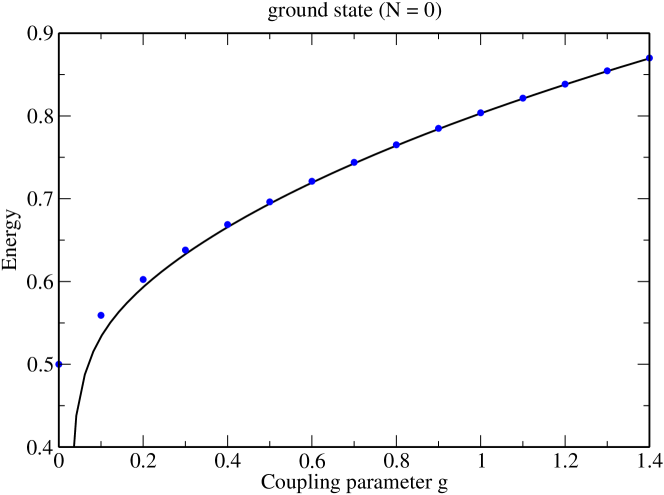
Figure 4: Exact values (filled circles) for the ground state energy of the quartic anharmonic oscillator as a function of $g$, together with the partial sum of the strong–coupling expansion (solid line) as defined by the first three nonvanishing terms in powers of $g^{-2k/3}$ [see Eq. (247)].

3.5 Odd Anharmonic Oscillators

Mathematical Discussion of odd anharmonic oscillators. The odd anharmonic oscillators in dimension $N$ (or, equivalently, in $N$ degrees of freedom) are by definition the anharmonic oscillators such that the potential $V_{\ell}$ in the Hamiltonian (229) is a polynomial in $N$ variables of odd degree $2s+1$, $s=1,2,\ldots$. The most famous example is probably the potential $V\equiv q_{1}^{2}\,q_{2}$, yielding the two-dimensional Hénon-Heiles Hamiltonian

$${\cal H}=\frac{1}{2}\,\left(p_{1}^{2}+p_{2}^{2}\right)+\omega_{1}^{2}\,q_{1}^{2}+\omega_{2}^{2}\,q_{2}^{2}+g\,q_{1}^{2}\,q_{2}\,,$$ (248)

which represents one of the fundamental models for the onset of chaos in classical Hamiltonian mechanics.

The basic difference to the even case is that here constant energy surfaces are in general not compact. Then the classical motions reach infinity when the initial conditions belong to open regions in phase space, and actually do it in a finite time. The quantum aspect of this mechanical property is the lack of self-adjointness of the corresponding Schrödinger operator, and consequently the lack of uniqueness of quantum dynamics. To better understand this point, consider the simplest one-dimensional case, the cubic anharmonic oscillator, whose Hamiltonian is (in an appropriate normalization):

$$H_{\ell=3}=p^{2}+q^{2}+g\,q^{3}\,.$$ (249)

The potential $V_{\ell=3}(q)=q^{2}+g\,q^{3}$ has a minimum at $q=0$ with value $V_{3}(0)=0$ and a maximum at $q=-2/3g$ with value $V_{3}(-2/3g)=\frac{4}{27g^{2}}$. Therefore, all classical trajectories with initial conditions fulfilling $E>\frac{4}{27g^{2}}$ reach $-\infty$ in a finite time (with at most one inversion of velocity) because the time required is well known to be

$$t=\int_{q_{0}}^{-\infty}\frac{dq}{\sqrt{E-q^{2}-g\,q^{3}}}$$ (250)

and this integral is convergent. Under these conditions (the classically incomplete case: see e.g. [44]) the corresponding Schrödinger operator $p^{2}+q^{2}+g\,q^{3}$ is not essentially self-adjoint because there are infinitely many different ways in which it can be realized as a self-adjoint operator in the Hilbert space $L^{2}({\mathbbm{R}})$. On the other hand the Rayleigh-Schrödinger perturbation theory exists. Actually the perturbation theory of the cubic anharmonic oscillator represents the very first problem considered by Heisenberg with matrix mechanics: see e.g. Ref. [223], and the first obvious question is to isolate the quantity to associate with it.

We consider this problem only in one dimension, and for a general interaction of the type $q^{2s+1}$, i.e. we consider the Schrödinger operators

$$H_{2s+1}(g)\equiv p^{2}+q^{2}+g\,q^{2s+1},\quad s=1,2,3\ldots,$$ (251)

The lack of self-adjointness for $g\neq 0$ entails a fortiori the instability of the harmonic oscillator eigenvalues. The asymptotic power series $E(g)\sim\sum_{n=0}^{\infty}a_{n}\,g^{n}$ generated by Rayleigh-Schrödinger perturbation theory near any unperturbed eigenvalue $E=a_{0}$ has indeed the following properties:

1. It contains only even powers; namely, $a_{2n+1}=0$. This is because the unperturbed operator is even under the parity operation $(P\psi)(q)=\psi(-q)$, and the perturbation is odd.

2. The nonzero coefficients $a_{2n}$ have constant sign, the perturbation series is nonalternating.

3. The even coefficients behave as $a_{2n}\sim(sn)!$ for $n\to\infty$.

The proof is given in Ref. [224]. If the series has only even powers of constant sign, the series $\sum_{n=0}^{\infty}a_{n}\,({\rm i}\,g)^{n}$ has alternating signs. It is thus conceivable that, in examining the summability properties of Rayleigh-Schrödinger perturbation theory, the natural starting point should be the examination of the operator $H_{2s+1}(g)$ for $g$ complex instead of $g$ real. One has indeed

Theorem 11

Let $H_{2s+1}(g)$ be the Hamiltonian of an odd anharmonic oscillator as discussed. It follows:

1. If $|{\rm arg}\,\beta|<\frac{\pi}{2}$, the operator $H_{2s+1}({\rm i}\,\beta)$ can be realized in a unique way as a closed operator in $L^{2}({\mathbbm{R}})$ with discrete spectrum; moreover $(H_{2s+1})^{\ast}({\rm i}\,\beta)=H_{2s+1}(-{\rm i}\,\overline{\beta})$, where $\overline{\beta}$ denotes the complex conjugate of $\beta$.

2. The eigenvalues of the unperturbed operator $H_{0}$ are stable as eigenvalues $E({\rm i}\,\beta)$ of the argument ${\rm i}\,\beta$ for $|\beta|$ small and $|{\rm arg}\,\beta|<\frac{\pi}{2}$; that is, if $E_{0}$ is any eigenvalue of the one-dimensional harmonic oscillator (and hence simple) there is $B(E_{0})>0$ such that $H({\rm i}\,\beta)$ has exactly one eigenvalue $E({\rm i}\,\beta)$ near $E_{0}$ for $|\beta|<B(E_{0})$ and $|{\rm arg}\,\beta|<\frac{\pi}{2}$.

3. Any eigenvalue $E({\rm i}\,\beta)$ is a holomorphic function of $\beta$ in the region $\{\beta:\,\,0<|\beta|<B(E_{0})\,;\,|{\rm arg}\,\beta|<\frac{\pi}{2}\}$; the function $E({\rm i}\,\beta)$ admits an analytic continuation to any sector $S_{\delta}=\{\beta\,:\,0<|\beta|<B_{\delta}(E_{0})\,;\,-\frac{\pi\,(2s-1)}{8}+\delta<{\rm arg}\,\beta<\frac{\pi\,(2s+7)}{8}-\delta\}$, $\forall\,\delta>0$ on a $(2s+3)$-sheeted Riemann surface.

4. The function $E({\rm i}\,\beta)$ and the Rayleigh-Schrödinger perturbation series fulfill the conditions of the Watson-Nevanlinna Theorem 5 in any sector $\{\beta\,:\,0\leq|\beta|<B_{\delta}(E_{0})\,,\,-\frac{\pi(2s-1)}{8}+\delta<{\rm arg}\,\beta<\frac{\pi(2s+7)}{8}-\delta\}$, $\forall\delta>0$.

5. The Rayleigh-Schrödinger perturbation series is Borel summable to $E({\rm i}\,\beta)$ in any sector $\{\beta\,:\,0\leq|\beta|<B_{\delta}(E_{0}),\,\,|{\rm arg}\,\beta|<\frac{\pi}{2}-\delta\}$, $\forall\delta>0$ or equivalently, to $E(g)$ in any sector $\{|g|<B_{\delta}(E_{0})\,;\,\delta<{\rm arg}\,g<\pi-\delta\}$, if we set $g={\rm i}\,\beta$.

Proof. These results are proven in [189, 190].

The above results clarify the meaning of the perturbation series as long as the summation is performed along nonreal directions; if the Borel sum is continued to $g$ real the result is a complex function. The question thus arises of establishing the relation between this complex-valued function and the real-valued perturbation series, and of finding the meaning of the imaginary part. The physical intuition is that this complex valued function should represent a resonance of the problem, even though there is no continuous spectrum involved: the real part should be the position, and the imaginary part the width, because it should be proportional to the penetration of the barrier. The distributional Borel summability puts on a rigorous basis this intuition. Namely we have:

Theorem 12

Let $E(g)$ be the analytic continuation to ${\rm Im}\,g=0$ of the function $E(g)$, which exists by the above Theorem. Then:

1. $E(g)$ and the perturbation series $\sum_{n=0}^{\infty}a_{n}\,g^{n}$ fulfill the conditions of the distributional Nevanlinna-Leroy criterion (see Theorem 21 and Definition 22 in Appendix B) of order $\frac{2s-1}{2}$.

2. The divergent perturbation series $\sum_{n=0}^{\infty}a_{n}\,g^{n}$ is Borel summable in the distributional sense of order $s$ to $E(g)$ for $|g|$ suitably small. Moreover, ${\rm Re}\,E(g)$ is even in $g$ and ${\rm Im}\,E(g)$ is odd.

Proof. See Ref. [225].

A few remarks are in order. (i) Equation (1.6) of Ref. [225] clarifies the role of the standard WKB analysis to the barrier penetration and the imaginary part ${\rm Im}\,E(g)$, in the context of odd anharmonic oscillators. (ii) The analogue of Theorem 12 for the Hénon-Heiles Hamiltonian (3.4.1) and for the ground state energy level of the harmonic oscillator has been recently proven in Ref. [226]. (iii) Consider the odd oscillators for purely imaginary values of the coupling $g$, i.e. the operators $H({\rm i}\,\beta)$, $\beta\in{\mathbbm{R}}$. Let $P$ be the standard parity operation: $(P\psi)(x)=\psi(-x)$, and $T$ the time-inversion operation, equivalent, as we know, to complex conjugation: $(T\psi)(x)=\overline{\psi}(x)$. $P$ and $T$ are unitary operations, and so is their product $PT=TP$. Now it is immediate to check that

$$[H({\rm i}\,\beta),PT]=[H({\rm i}\,\beta),TP]=0\,,$$ (252)

i.e. the odd anharmonic oscillators are examples of $PT$-symmetric operators. It has been conjectured around 1985 by Bessis and Zinn-Justin that the spectrum of the odd $PT$-symmetric anharmonic oscillators should consist of real eigenvalues for all values of $\beta\in{\mathbbm{R}}$, even if the operator $H(\beta)$ is obviously not self-adjoint and not even normal because it is easily verified that $[H({\rm i}\,\beta),H({\rm i}\,\beta)^{\ast}]=[H({\rm i}\,\beta),H(-{\rm i}\,\beta)]\neq 0$. Note that by the Borel summability the reality of the spectrum is valid for $\beta$ small (depending on the eigenvalue index $k$) because the eigenvalues of the harmonic oscillators are stable for $\beta$ small and the perturbation series for each eigenvalue is real when $g={\rm i}\,\beta$, $\beta\in{\mathbbm{R}}$. Notice that in this general setting, the non-normality makes also the problem of the existence of eigenvalues a nontrivial problem in situations where perturbation theory cannot be applied, such as the one obtained for $\beta$ large. Later Bender (Ref. [227]) conjectured that $PT$-symmetric Hamiltonians should always have real spectrum, so that $PT$-symmetry could be considered a condition equivalent to self-adjointness in ensuring the reality of the spectrum as long as Schrödinger operators are concerned. This latter conjecture has been disproven [228], but the original Bessis-Zinn-Justin conjecture has been recently proven by Shin [229] (see also Refs. [230, 231, 232]).

Theorem 13

Let $H_{2s+1}(g)$ be the Hamiltonian of the one-dimensional odd anharmonic oscillator. For any $s\in{\mathbbm{N}}$ and any $g={\rm i}\,\beta$, $\beta\in{\mathbbm{R}}$, the spectrum of the operator $H_{2s+1}(g)$ consists of countably many simple positive eigenvalues $E_{N}({\rm i}\,\beta)$.

Proof. See Shin [229].

Finally, we note that similar results as for anharmonic oscillators hold for the resonances of the Stark effect, see Appendix B.2.

Practical resummations and complex scaling of eigenvalues for the cubic potential. As for the even anharmonic oscillators, we now supplement the mathematically inspired analysis by some concrete calculations.

Before starting the numerical analysis of the cubic potential, however, we may mention that the problem of “recovering” the complex resonance energies from a nonalternating perturbation series has been discussed for the Stark effect in [207, 209] and for the quantum electrodynamics (QED) effective action in [208]. For the Stark effect, for example, the situation is as follows: the problem is spectrally unstable: as soon as the electric field is turned on, all eigenvalues of the hydrogen atom disappear in the continuous spectrum (a phenomenon first proven by Titchmarsh [233]). Thus the perturbation theory is always divergent. The physical reason is that the linear potential of the electric field generates a tunneling phenomenon. As first pointed out by Oppenheimer [234], the hydrogen eigenvalues are thus expected to turn into resonances: their width (inverse life-time) should be proportional to the probability of penetrating the barrier. In the 1970s and 1980s, this picture has been set on rigorous mathematical grounds: moreover, the perturbation theory of the problem has fully been understood. Not only it can be uniquely associated with the resonances via ordinary and distributional Borel summability, but it defines very effective approximation schemes for computing both the location and the width of the resonances.

Here, we can rely on the literature for the Stark effect and for the QED effective action and treat the conceptually simpler case of the cubic anharmonic oscillator as an example. Calculations for such a potential will be performed in order to illustrate how to derive the complex resonance eigenvalues (including the width) from a real perturbation series using Borel summation in complex directions of the parameters, in the sense of distributional Borel summability. We discuss the problem of determination of the complex resonance energies for the case of the cubic oscillator, in the normalization:

$$H(g)=\frac{p^{2}}{2}+\frac{q^{2}}{2}+\sqrt{g}\,q^{3}\,.$$ (253)

The energy spectrum of the anharmonic oscillator can be analyzed numerically, e.g. via a diagonalization of the Hermitian matrix within a (large) basis of harmonic oscillator wavefunctions. One has to take into account, though, that the bound states of the (odd) harmonic oscillator become resonances, labeled by an index $N$ according to the above Theorems 11 and 12:

$$E_{N}(g)={\rm Re}\,E_{N}(g)-{\rm i}\,\frac{\Gamma_{N}(g)}{2}\,,$$ (254)

where $\Gamma_{N}(g)$ is the width. An appropriate ansatz for studying the energy spectra of the odd anharmonic oscillators has been proposed in Refs. [191] and [235] and is based on the complex (or so-called dilation) transformation of the coordinate $q$:

$$q\mapsto q\,{\rm e}^{{\rm i}\,\theta}\,,$$ (255)

where $\theta$ may be real or complex. By inserting this transformed coordinate into Eq. (253), we may obtain the complex-scaled Hamiltonian for the cubic oscillator:

$$H(g,\theta) = -\frac{1}{2}\frac{d^{2}}{dq^{2}}{\rm e}^{-2{\rm i}\theta}+\frac{q^{2}}{2}{\rm e}^{2{\rm i}\theta}+\sqrt{g}\,q^{3}{\rm e}^{3{\rm i}\theta}$$ (256)

$$= {\rm e}^{-2{\rm i}\theta}\left(-\frac{1}{2}\frac{d^{2}}{dq^{2}}+\frac{q^{2}}{2}{\rm e}^{4{\rm i}\theta}+\sqrt{g}\,q^{3}{\rm e}^{5{\rm i}\theta}\right)\,.$$

As discussed in Ref. [235], by finding the eigenvalues of this dilationally transformed Hamiltonian one may find that when $\theta$ becomes large enough, one of the rotated branches passes the position of a resonance pole, and a new eigenvalue of the Hamiltonian (256) appears at the position of the resonance pole. This resonance eigenvalue, once uncovered, remains fixed in the complex plane and is independent of further increases in $\theta$. Hence, the evaluation of the eigenvalues of the Hamiltonian (256) allows us to determine the (complex) energies of the original cubic Hamiltonian (253).

Now we are ready to calculate the energy values of the complex–transformed (256) and, hence, of the original cubic Hamiltonian (253). Again, these calculations can be performed via matrix diagonalization in the basis of harmonic oscillator wavefunctions. The result of such diagonalization procedure for a coupling parameter $g=0.01$ is presented in the last line of the Table 9 and is found in perfect agreement with previous calculations [236].

We not study the resummation of the perturbation series within the complex plane. In order to discuss this resummation procedure let us again recall that within the standard Rayleigh–Schrödinger perturbation approach, the eigenvalues of the cubic potential are given by the series

$$E_{N}=N+\frac{1}{2}+\sum\limits_{k=1}^{\infty}A_{N}^{k}g^{k}\,,$$ (257)

where the first six perturbation coefficients for the ground state $N$ = 0 are:

$$A_{0}^{1} = -\frac{11}{8}\,,\quad A_{0}^{2}=-\frac{456}{32}\,,\quad A_{0}^{3}=-\frac{39709}{128}\,,$$

$$A_{0}^{4} = -\frac{19250805}{2048}\,,\quad A_{0}^{5}=-\frac{2944491879}{8192}\,,\quad A_{0}^{6}=-\frac{1075012067865}{65536}\,.$$ (258)

Similar to the case of the quartic oscillator, this series is divergent and, hence, its term–by–term summation cannot reproduce the energy values of the cubic potential. Apart from such a non–summability, moreover, another problem should be mentioned. Namely, no complex part (i.e. width) of the eigenvalues can be obtained by straightforward summation of Eq. (257). We may calculate these widths, however, if we apply the Borel–Padé resummation method with an integration contour deformed into the complex plane as discussed in Eqs. (241)–(243). For such an integration, however, we have to choose the proper contour in the complex plane in order to reproduce the correct sign for the imaginary part of the energy. In our calculations for the cubic potential, for example, the contour $C_{-1}$ has been chosen because it leads to the correct negative sign of the imaginary part of the resonance energy eigenvalue. Notice that the distributional Borel summability also does not fix the sign of imaginary part on the basis of the purely real perturbation series (see Theorem 12), and the choice of the contour has to be inserted based on an “external,” physical consideration. As seen from the third column of the Table 9, the Borel–Padé method allows us to reproduce the complex resonance energy of the ground state of cubic potential for a coupling parameter $g=0.01$.

Table 9: Resummation of the asymptotic series (239) taken at $g=0.01$ for the ground-state energy of the cubic anharmonic oscillator (253). In the first row, we indicate the quantity $n$ which is the order of the perturbation expansion. In the second row, we list the partial sums $s_{n}=\sum^{n}_{k=0}A_{0}^{k}g^{k}$ of the purely real perturbation theory, whereas in the fourth row, the Borel–Padé transformation is presented [cf. Eqs. (241)–(243)].

n	$\sum^{n}_{k=0}A_{0}^{k}g^{k}$	${\mathcal{T}}\!{\mathcal{P}}_{n}(g)$
$1$	$\underline{0.48}6~{}250~{}000$	$\underline{0.48}6~{}949~{}910-\underline{0.000~{}00}0~{}000\,{\rm i}$
$2$	$\underline{0.484}~{}796~{}875$	$\underline{0.484}~{}497~{}987-\underline{0.000~{}00}0~{}093\,{\rm i}$
$3$	$\underline{0.484}~{}486~{}648$	$\underline{0.484~{}3}41~{}583-\underline{0.000~{}00}4~{}008\,{\rm i}$
$4$	$\underline{0.484~{}3}92~{}650$	$\underline{0.484~{}315}~{}106-\underline{0.000~{}0}10~{}069\,{\rm i}$
$5$	$\underline{0.484~{}3}56~{}707$	$\underline{0.484~{}315}~{}279-\underline{0.000~{}00}9~{}966\,{\rm i}$
$...$	$\underline{}...$	$\underline{}...$
$10$	$\underline{0.484~{}3}20~{}462$	$\underline{0.484~{}31}6~{}006-\underline{0.000~{}008~{}0}57\,{\rm i}$
$11$	$\underline{0.484~{}31}8~{}395$	$\underline{0.484~{}31}6~{}001-\underline{0.000~{}008~{}0}52\,{\rm i}$
$12$	$\underline{0.484~{}31}6~{}573$	$\underline{0.484~{}315~{}99}9-\underline{0.000~{}008~{}0}58\,{\rm i}$
$13$	$\underline{0.484~{}31}4~{}836$	$\underline{0.484~{}315~{}99}8-\underline{0.000~{}008~{}0}58\,{\rm i}$
$14$	$\underline{0.484~{}31}3~{}053$	$\underline{0.484~{}315~{}99}9-\underline{0.000~{}008~{}0}59\,{\rm i}$
$15$	$\underline{0.484~{}31}1~{}093$	$\underline{0.484~{}315~{}997}-\underline{0.000~{}008~{}060}\,{\rm i}$
$16$	$\underline{0.484~{}3}08~{}792$	$\underline{0.484~{}315~{}997}-\underline{0.000~{}008~{}060}\,{\rm i}$
exact	$0.484~{}315~{}997$	$0.484~{}315~{}997-0.000~{}008~{}060\,{\rm i}$

3.6 Double–Well and Fokker–Planck Potential

Mathematical discussion of double-well like potentials. Let us restrict ourselves to the discussion of the one-dimensional case. The simplest example is represented by the symmetric double-well Hamiltonian, which reads (in an appropriate normalization)

$$H^{\rm DW}(g)=p^{2}+q^{2}(1-g\,q)^{2}$$ (259)

The translation $q\mapsto q+1/2g$ maps the Hamiltonian to the form $p^{2}+g^{2}(q+1/2g)^{2}(q-1/2g)^{2}$ which is manifestly an even function with two symmetric quadratic minima at $q=\pm 1/2g$. The Hamiltonian (259) has minima at $q=0$ and $q=1/g$ and the second one disappears as $g\to 0$.

Within even anharmonic oscillators examples exhibiting spectral instability have a special status and a typical examples is just the double-well oscillator. As already mentioned, the basic phenomenon in this context is the spectral instability, or, equivalently, asymptotic degeneracy of the eigenvalues. For the symmetric double well, the well known physical picture goes as follows (see e.g. [237]): in classical mechanics the two wells are identical, and therefore generate the same motions, in the sense that the phase curves in the two separate wells are the same. Quantum mechanics just adds to this picture the tunneling phenomenon. Therefore we may expect to find, for $g$ small, a doublet of eigenvalues of the double well operator $H^{\rm DW}(g)$ close to each unperturbed eigenvalue $E$, and therefore $E$ is unstable. The first mathematical proof of this picture is due to Harrell [238] who showed that as $|g|\to 0$, there are exactly two eigenvalues $E_{\pm}(g)$ of $H^{\rm DW}(g)$ near any unperturbed eigenvalue $E$, and that the Rayleigh-Schrödinger perturbation expansion is an asymptotic expansion for both eigenvalues of the doublet.

As we have seen, to understand the meaning of perturbation theory, it is in general necessary to understand the analyticity property of the eigenvalues for complex values of the coupling constant $g$. In the case of only a single well, this is possible thanks to the stability of the eigenvalues even for complex values of the coupling constant. It is remarkable that also in the unstable case of the double-well, one can identify and construct a pair of operators $H_{\pm}(g)$, the so-called single well operators which admit $E_{\pm}(g)$ as stable eigenvalues as $g\to 0$ in a suitable complex region. The operators $H_{+}(g)$ and $H_{-}(g)$ are obtained by projecting orthogonally $H(g)$ onto the subspace of the even and odd functions with respect to the top of the barrier at $x=1/2g$, respectively. This represents the mathematical justification of the physical intuition that the two perturbed quantum states “live” in two separate but equal wells, and makes it possible to perform the stability analysis as already mentioned. The result is

Theorem 14

Consider the double well operator $H^{\rm DW}(g)$.

1. $\exists R>0$ so that both eigenvalues $E_{\pm}(g)$ are analytic in the Nevanlinna disk $C_{R}\equiv\{g:{\rm Re}\,g^{-2}>R^{-1}\}$.

2. The eigenvalues $E_{\pm}(g)$ are stable near the eigenvalue $E$ of the unperturbed problem as $|g|\to 0$, $g\in C_{R}$, if considered as eigenvalues of the operators $H_{\pm}(g)$, respectively.

Proof. See [239, 240, 190].

The summability statement for the perturbation theory can hold only in an indirect way, identified in [240]. Two further operators have to be associated with the differential expression $p^{2}+q^{2}(1-g\,q)^{2}$, namely the resonance operators $T_{\pm 1}(g)$. The operator $T_{+1}(g)$ is defined by the the differential expression $p^{2}+q^{2}(1-q\,q)^{2}$ by modifying the $L^{2}$ boundary condition at $+\infty$: the functions in its domain are required to be entire analytic and vanish as $|q|\to+\infty$ within the sector $S_{1}\equiv\{q\in{\mathbbm{C}}:\frac{\pi}{6}<{\rm arg}\,q<\frac{\pi}{2}\}$. Analogously, the operator $T_{-1}(g)$ is defined by the vanishing boundary condition in the symmetrical sector $S_{-1}\equiv\{x\in{\mathbbm{C}}:-\frac{\pi}{2}<{\rm arg}\,x<-\frac{\pi}{6}\}$. These considerations allow us to express the matrix elements of the resolvent of $H^{\rm DW}(g)$ as linear combinations of those of $T_{\pm 1}$.

We now define various projection operators. Let

$$P_{\pm}(g)\,\psi(x)=\frac{1}{2}\,\left[\psi(x)\pm\psi(g^{-1}-x)\right]\,,\qquad\psi\in L^{2}(\mathbbm{R})\,,$$ (260)

represent the projections onto the subspaces of the even (respectively odd) functions with respect to the barrier point $x=1/2g$. Then, $H^{\rm DW}_{\pm}(g)=P_{\pm}(g)\,H^{\rm DW}(g)\,P_{\pm}(g)$. We also define the following projectors,

$$Q(g)= \;2\pi{\rm i}-\oint_{|z-E|=r}\frac{1}{z-H^{\rm DW}(g)}{\rm d}z\,,$$ (261a)

$$Q_{\pm}(g)= \;2\pi{\rm i}-\oint_{|z-E|=r}\frac{1}{z-H^{\rm DW}_{\pm}(g)}{\rm d}z\,.$$ (261b)

These project out those eigenfunctions of $H^{\rm DW}(g)$ and $H^{\rm DW}_{\pm}(g)$ whose energies $E_{n}$ fulfill $|E_{n}-E|<r$. Let $\psi_{0}$ be the unperturbed eigenvector corresponding to $E$. With the convention $\psi_{\pm}=P_{\pm}(g)\,\psi_{0}$, we now define the expressions

$$N_{\pm}(g)= \;\left<\psi_{0}\left|H^{\rm DW}_{\pm}(g)\,Q_{\pm}(g)\right|\psi_{0}\right>\;=\;\left<\psi_{\pm}\left|H^{\rm DW}(g)\,Q(g)\right|\psi_{\pm}\right>\,,$$ (262a)

$$D_{\pm}(g)= \;\left<\psi_{0}\left|Q_{\pm}(g)\right|\psi_{0}\right>\;=\;\left<\psi_{\pm}\left|Q(g)\right|\psi_{\pm}\right>\,.$$ (262b)

By standard Rayleigh-Schrödinger perturbation theory, we can now write any double well eigenvalue $E_{\pm}(g)$ under the form

$$E_{\pm}(g)=\frac{N_{\pm}(g)}{D_{\pm}(g)}=\frac{\left<\psi_{\pm}\left|H^{\rm DW}(g)\,Q(g)\right|\psi_{\pm}\right>}{\left<\psi_{\pm}\left|Q(g)\right|\psi_{\pm}\right>}\,.$$ (263)

If we restrict our attention now to a specific manifold of states with a definite parity, then we may write the energy eigenvalue of the symmetric double-well as

$$E(g)=\frac{N(g)}{D(g)}\,.$$ (264)

Following Ref. [240], it is possible to prove a representation formula of the type

$$N(g)=\frac{1}{2}[\Phi(g)+\overline{\Phi}(g)]$$ (265)

and analogously for $D(g)$, $g\in C_{R}$. Then one proves:

Theorem 15

With the above definitions, we have the assertions:

1. The function $\Phi(g)$ admits a power series expansion in $g$; $\Phi(g)$ and its expansion fulfill the conditions of Theorem 21 (see Appendix B). More precisely:

2. The power series expansion is Borel summable in the distributional sense (see Definition 20, Theorem 21 and the remark after it) i.e.: $\Phi(g)$ is the upper sum, $\overline{\Phi}(g)$ is the lower sum, $N(g)$ is the distributional Borel sum, and $\Phi(g)-\overline{\Phi}({g})$ is the discontinuity.

3. An analogous statement holds for $D(g)$ and its perturbation expansion.

Proof. See [240].

Let us add a couple of remarks concerning the effect that the asymptotic degeneracy phenomenon and the related tunneling are fragile, i.e. they critically depend on the exact symmetry. Indeed these phenomena disappear when the the symmetry is broken even by an infinitesimal amount. The following two observations can be made. (i) Consider for example the Schrödinger operator $H_{g,\epsilon}=p^{2}+q^{2}-2g(1+\epsilon)q^{3}+g^{2}\,q^{4}$, $\epsilon>0$ which corresponds to shifting the second minimum up by $\epsilon$ from $0$. Then the unperturbed eigenvalues are stable and the perturbation expansion near any unperturbed eigenvalue is Borel summable (for the proof, see [241]). (ii) Suppose we perform an arbitrarily small variation of the profile of the potential $q^{2}(1-gq)^{2}$ away from the minima. Then the constant $A$ changes by a finite amount, so that the tunneling probability changes by several orders of magnitudes (see for instance [217, 242]). The latter observation has been termed the “flea over the elephant” by Simon in Ref. [243].

A remarkable example by Herbst and Simon [244] shows that this phenomenon takes place even within perturbation theory of stable, but asymmetric multi-well anharmonic oscillators. Consider indeed the following Schrödinger operator

$$H_{\rm FP}(g)=p^{2}+q^{2}\,(1-g\,q)^{2}+2g\,q-1\,,$$ (266)

where the symmetry of the minima is broken by the linear term. This symmetry breaking makes the unperturbed eigenvalues stable; however the Rayleigh-Schrödinger perturbation theory for the ground state $E(g)$ is identically zero, while $E(g)$ itself is not zero.

This problem finds a natural solution here within the context of resurgent expansions and has also been treated in [240], where a general Schrödinger operator is examined of the type

$$H(g,j)=p^{2}+q^{2}(1-gq)^{2}-j(gq-1/2)\,,$$ (267)

which reduces to the symmetrical double well for $j=0$ and to the Fokker–Planck Hamiltonian [244, 181] for $j=-2$. The precise mathematical statement of the solution is too technical to be reproduced here. Roughly speaking, however, the results are as follows:

(i) If $j\neq 2p$, $p=0,\pm 1,\ldots$, the same results as Theorem 15 hold. More precisely, the eigenvalues of $H(g,j)$ split into two disjoint subsets $\{E_{N}(g,j)\}$ and $\{E^{\prime}_{N}(g,j)\}$. The eigenvalues $\{E_{N}(g,j)\}$ are stable near the eigenvalues $2N+1+j/2$ of $H(g,j)$, the harmonic oscillator up to the shift $j/2$; The eigenvalues $\{E^{\prime}_{N}(g,j)\}$ converge to $2N+1-j/2$ and therefore have nothing to do with the limiting problem. They are instead stable with respect to another limiting problem at $g=0$, namely the harmonic oscillator up to the shift $-j/2$. The eigenvalues $E_{N}(g,j)$ admit a Borel summable perturbation expansion, while the perturbation expansion for any single eigenvalue $E^{\prime}_{N}(g,j)$ is identically zero. (ii) If $j=2p$, $p=\pm 1,\pm 2\ldots$ an eigenvalue of the first limiting problem may coincide with an eigenvalue of the second one. Therefore a $2\times 2$ matrix has to be introduced, with elements still defined in terms of matrix elements of the resolvents of the corresponding single well operators. The two perturbed eigenvalues are the eigenvalues of this matrix. The coefficients of the matrix have expression analogous to (265), and are likewise Borel summable in the distributional sense.

Practical resummations of double-well like potentials. We start from the case of the symmetric double–well potential, this time in the normalization:

$$H_{\rm dw}(g)=\frac{1}{2}\,p^{2}\,+\,\frac{1}{2}q^{2}\left(1-\sqrt{g}\,q\right)^{2}\,=\frac{p^{2}}{2}\,+\,\frac{q^{2}}{2}\,-\,\sqrt{g}\,q^{3}\,+\,g\frac{q^{4}}{2},$$ (268)

where, again, $g$ is a real, positive coupling parameter. Obviously, if $g\,=\,0$, then Eq. (268) represents the Hamiltonian of the quantum harmonic oscillator whose eigenvalues are given by the well known formula $E_{N}\,=\,N+1/2$, where $N\in\mathbb{N}_{0}$ is the principal quantum number. For nonvanishing coupling, by contrast, no analytic expression for the energies $E_{N}(g\neq 0)$ can be derived and, hence, approximate methods have to be applied for solving Eq. (268). First, we again start from the Rayleigh–Schrödinger perturbation theory which allows us to write the perturbation series (239) series for the energy values $E_{N}(g)$. For the ground state $N=0$, the first six coefficients $A_{N=0}^{k}$ of these series are given by (see, e.g., [85]):

$$A_{0}^{1} = -1\,,\quad A_{0}^{2}=-\frac{9}{2}\,,\quad A_{0}^{3}=-\frac{89}{2}\,,$$

$$A_{0}^{4} = -\frac{5013}{8}\,,\quad A_{0}^{5}=-\frac{88251}{8}\,,\quad A_{0}^{6}=-\frac{3662169}{16}\,.$$ (269)

As in the case of the cubic anharmonic oscillator (3.5), these coefficients grow factorially and have the same sign. The perturbation series (239) with these coefficients are, hence, divergent and not Borel–summable. As mentioned already in the discussion above, however, apart from the non-summability of the series (239) another and even more critical argument against the application of the Rayleigh–Schrödinger perturbation theory to the double–well potential has been mentioned [245, 178, 246, 247, 181, 179, 180]. Namely, while the perturbation series (239), if being resummed, would provide only one energy level for every quantum number $N$, two eigenstates are known to appear in the case of nonvanishing coupling $g>0$. Such a splitting of the level of the unperturbed Hamiltonian into two levels (the instability of the eigenvalues from a mathematical point of view) has been explained by Landau and Lifshitz [237] within a semiclassical WKB approach and has been attributed to the effect of quantum tunneling through the potential barrier between the two wells. However, while the semiclassical approach has provided a qualitative and perhaps semi-quantitative understanding of the energy spectrum, it can hardly be extended for a full and accurate quantitative analysis of the double–well (as well as multi–well) potentials.

Table 10: Energy splitting between the ”ground” states $E_{0,\varepsilon=\pm 1}(g)$ of the double–well Hamiltonian at the coupling parameter $g$ = 0.005. In the first row, we indicate the quantity $n$ which is the order of the expansion (275). In the second row, we list the partial sums (275), whereas in the third row, the Borel–Padé transformation is presented [cf. Eqs. (241)–(243)].

$n$	$2\,\frac{{\rm e}^{-1/6g}}{\sqrt{\pi g}}\sum^{n}_{l=0}e_{0,10l}\,g^{l}$	${\mathcal{T}}\!{\mathcal{P}}_{n}(g)$
$0$	$\underline{5}.327~{}056~{}794\times 10^{-14}$	$\underline{}$
$1$	$\underline{5.16}9~{}464~{}698\times 10^{-14}$	$\underline{5.1}78~{}046~{}952\times 10^{-14}$
$2$	$\underline{5.166}~{}551~{}926\times 10^{-14}$	$\underline{5.166}~{}468~{}039\times 10^{-14}$
$3$	$\underline{5.166~{}3}79~{}090\times 10^{-14}$	$\underline{5.166~{}36}7~{}389\times 10^{-14}$
$4$	$\underline{5.166~{}36}4~{}871\times 10^{-14}$	$\underline{5.166~{}363}~{}195\times 10^{-14}$
$5$	$\underline{5.166~{}363}~{}450\times 10^{-14}$	$\underline{5.166~{}363~{}2}50\times 10^{-14}$
$6$	$\underline{5.166~{}363~{}2}86\times 10^{-14}$	$\underline{5.166~{}363~{}26}2\times 10^{-14}$
$7$	$\underline{5.166~{}363~{}26}5\times 10^{-14}$	$\underline{5.166~{}363~{}261}\times 10^{-14}$
$8$	$\underline{5.166~{}363~{}26}2\times 10^{-14}$	$\underline{5.166~{}363~{}261}\times 10^{-14}$
$9$	$\underline{5.166~{}363~{}261}\times 10^{-14}$	$\underline{5.166~{}363~{}261}\times 10^{-14}$
exact	$5.166~{}363~{}261\times 10^{-14}$	$5.166~{}363~{}261\times 10^{-14}$

In this direction, an alternative route for studying the eigenvalues of the double–well–like potentials has been proposed and described in detail in Refs. [245, 178, 246, 247, 181, 179, 180] and is based on the Feynman path integral approach. We restrict ourselves here to a rather short account of the basic formulas. In particular, it has been conjectured that the eigenvalues of the Hamiltonian (268) can be found by solving the generalized Bohr–Sommerfeld quantization condition

$$\frac{1}{\sqrt{2\pi}}\Gamma\left(\frac{1}{2}-B_{\rm dw}(E,g)\right)\,\left(-\frac{2}{g}\right)^{B_{\rm dw}(E,g)}\,{\rm exp}\left[-\frac{A_{\rm dw}(E,g)}{2}\right]\,=\,\varepsilon i\,,$$ (270)

where $\varepsilon=\pm 1$ is the parity, and the functions $B_{\rm dw}(E,g)$ and $A_{\rm dw}(E,g)$ are determined by the perturbative expansion and the perturbative expansion about the instantons, respectively. The evaluation of these functions in terms of series in variables $E$ and $g$ has been described in detail elsewhere [179, 180, 247] for quite general classes of potentials. For the particular case of the double–well potential, for example, the function $B_{\rm dw}(E,g)$ has the following expansion:

$$B_{\rm dw}(E,g)\,=\,E\,+\,g\left(3E^{2}+\frac{1}{4}\right)\,+g^{2}\left(35E^{3}+\frac{25}{4}E\right)\,+\,\mathrm{O}(g^{3})\,,$$ (271)

and defines the perturbation expansion (239) which can be easily found by inverting the equation $B_{\rm dw}(E,g)\,=\,N$. The instanton contributions to the eigenvalues of the Fokker–Planck Hamiltonian are described by the function

$$A_{\rm dw}(E,g)\,=\,\frac{1}{3g}\,+\,g\left(17E^{2}+\frac{19}{12}\right)\,+\,g^{2}\left(227E^{3}+\frac{187}{4}E\right)\,+\,\mathrm{O}(g^{3})\,.$$ (272)

By making use of the generalized Bohr–Sommerfeld quantization condition (270) together with the expansions (271)–(272) of the $A_{\rm dw}$ and $B_{\rm dw}$ functions, we may finally derive the eigenvalues of the double–well Hamiltonian. That is, by expanding (270) in powers of the two small parameters $\exp(-1/6g)$ and $g$, the eigenvalues of the Hamiltonian (268) we may find a so–called generalized perturbation expansion (resurgent expansion)

$$E_{N,\varepsilon}(g)=\sum_{l=0}^{\infty}A^{l}_{N}\,g^{l}+\sum^{\infty}_{n=1}\left(\frac{2}{g}\right)^{Nn}\left(-\varepsilon\,\frac{{\rm e}^{-1/6g}}{\sqrt{\pi g}}\right)^{n}\,\sum^{n-1}_{k=0}\left\{\ln\left(-\frac{2}{g}\right)\right\}^{k}\,\sum^{\infty}_{l=0}e_{N,nkl}\,g^{l}\,,$$ (273)

which apart of the perturbation series also accounts for the instanton contributions. As seen from this expansion, apart from the principal quantum number $N$, eigenvalues of the double–well potential are characterized also by the parity $\varepsilon\,=\,\pm 1$. That is, each unperturbed level with the quantum number $N$ splits up into two states of opposite parity. Such a splitting is described by the second term in the right–hand side of the Eq. (273) and is attributed to the instanton contributions. The order of the instanton contribution is defined by the index $n$, with $n=1$ being the one–instanton contribution, etc. Despite of its name, the leading, one–instanton term involves a summation over all possible $n$-instanton configurations but neglects instanton interactions [179]. As seen from Eq. (273), the evaluation of the energies within such a (first-order) approximation, also referred as a “dilute instanton gas” approximation, requires the knowledge of the $e_{N,nkl}$ coefficients. Since these coefficients are available for download [85], we recall here just the six leading ones for the ground state $N=0$ of the double-well potential:

$$e_{0,100} = 1\,,\quad e_{0,101}=-\frac{71}{12}\,,\quad e_{0,102}=-\frac{6299}{288}\,,\quad e_{0,103}=-\frac{2691107}{10368}\,,$$ (274)

$$e_{0,104} = -\frac{2125346615}{497664}\,,\quad e_{0,105}=-\frac{509978166739}{5971968}\,,\quad e_{0,106}=-\frac{846134074443319}{429981696}\,.$$

By inserting these coefficients in Eq. (273), we are able to perform a numerical check of the validity of the one-instanton expansion for the energy splitting

$$\Delta E_{0}\,=\,E_{0,-1}-E_{0,1}\,\sim\,\left(2\,\frac{{\rm e}^{-1/6g}}{\sqrt{\pi g}}\right)\,\sum^{\infty}_{l=0}e_{0,10l}\,g^{l}$$ (275)

of the ground-state level $N$ = 0 due to the quantum tunneling. As seen from the second column of the Tables 10 and 11, however, a straightforward, term-by-term summation of the series (275) may well reproduce the energy splitting $\Delta E_{0}$ for the case of the small coupling $g=0.005$ but leads to the divergence of the result for strong coupling of $g=0.03$. In order to overcome such a divergence we again employ the Borel–Padé resummation method as given by Eqs. (241)–(243) in which as input data we used coefficients $e_{0,10l}$. However, while the Borel–Padé method provides a good convergence of the series (275), the result of resummation shows significant discrepancy with the “true” energy splitting as computed by the diagonalization of the Hamiltonian (268) in the basis of the harmonic oscillator wavefunctions. Such a discrepancy indicates the importance of the higher–instanton terms which take into account the instanton interactions for the case of strong coupling. The evaluation of the higher–order corrections ($n\geq$ 2) to the energies of the double–well potential is, however, a very difficult task since it requires a double resummation of the resurgent expansion, in powers of both $g$ and $\exp(-1/6g)$. In this contribution, one may address the question whether it is possible to resum the divergent series that gives rise to the $A_{\rm dw}$ and $B_{\rm dw}$ functions directly and look for solutions of the quantization condition (270) without recourse to the resurgent expansion. As it was discussed recently [248], this appears to be the only feasible way to evaluate the multi-instanton expansion (in power of $n$) because the quantization condition incorporates all instanton orders. We briefly summarize the results of this investigation here, which has been carried out for a potential closely related to the symmetric double-well.

Table 11: Energy splitting between the ”ground” states $E_{0,\varepsilon=\pm 1}(g)$ of the double–well Hamiltonian at the coupling parameter $g=0.03$. In the first row, we indicate the quantity $n$ which is the order of the expansion (275). In the second row, we list the partial sums (275), whereas in the third row, the Borel–Padé transformation is presented [cf. Eqs. (241)–(243)].

$n$	$2\,\frac{{\rm e}^{-1/6g}}{\sqrt{\pi g}}\sum^{n}_{l=0}e_{0,10l}\,g^{l}$	${\mathcal{T}}\!{\mathcal{P}}_{n}(g)$
$0$	$\underline{}2.518~{}531~{}055\times 10^{-2}$	$\underline{}$
$1$	$\underline{}2.071~{}491~{}792\times 10^{-2}$	$\underline{}2.178~{}799~{}750\times 10^{-2}$
$2$	$\underline{}2.021~{}916~{}083\times 10^{-2}$	$\underline{}2.011~{}031~{}238\times 10^{-2}$
$3$	$\underline{}2.004~{}265~{}988\times 10^{-2}$	$\underline{1.98}9~{}410~{}405\times 10^{-2}$
$4$	$\underline{}1.995~{}553~{}827\times 10^{-2}$	$\underline{1.983~{}5}47~{}787\times 10^{-2}$
$...$	$\underline{}...$	$\underline{}...$
$33$	$\underline{}-1.487~{}012~{}669\times 10^{2}$	$\underline{1.98}0~{}196~{}846\times 10^{-2}$
$34$	$\underline{}-4.525~{}128~{}589\times 10^{2}$	$\underline{1.98}0~{}196~{}848\times 10^{-2}$
$35$	$\underline{}-1.418~{}424~{}114\times 10^{3}$	$\underline{1.98}0~{}196~{}848\times 10^{-2}$
$36$	$\underline{}-4.575~{}754~{}388\times 10^{3}$	$\underline{1.98}0~{}196~{}848\times 10^{-2}$
exact	$1.983~{}530~{}115\times 10^{-2}$	$1.983~{}530~{}115\times 10^{-2}$

We discuss the main ideas of such a “direct summation” approach for the case of the so–called Fokker–Planck potential:

$$H_{\rm FP}(g) = \frac{1}{2}p^{2}\,+\,\frac{1}{2}q^{2}\left(1-\sqrt{g}q\right)^{2}\,+\,\sqrt{g}q\,-\,\frac{1}{2}$$ (276)

$$= \frac{1}{2}p^{2}\,+\,\frac{1}{2}q^{2}\,-\,\frac{1}{2}\,+\,\sqrt{g}q\,-\,\sqrt{g}q^{3}\,+\,\frac{g}{2}q^{4}\,,$$

which can be considered as a modification of the double–well potential (268). In contrast to the double–well case, however, the Fokker–Planck potential contains a linear symmetry–breaking term. Because of this term, the ground state of the potential (276) is located in one of the wells and, hence, does not develop any degeneracy due to parity (see also the mathematically inspired discussion earlier in this Section of the review). Excited states, however, can still be degenerate for $g\to 0$ in view of the (perturbatively broken) parity $\varepsilon\,=\,\pm 1$ of the quantum eigenstates. Again, in order to analyze such a degeneracy we may start from the generalized Bohr–Sommerfeld quantization condition which for the case of Fokker–Planck Hamiltonian reads as:

$$\frac{1}{\Gamma(-B_{\rm FP}(E,g))\Gamma(1-B_{\rm FP}(E,g))}\,+\,\left(-\frac{2}{g}\right)^{2B_{\rm FP}(E,g)}\frac{{\rm e}^{-A_{\rm FP}(E,g)}}{2\pi}\,=\,0\,,$$ (277)

where the series for the functions $B_{\rm FP}(E,g)$ and $A_{\rm FP}(E,g)$ are:

$$B_{\rm FP}(E,g)\,=\,E\,+\,3E^{2}g\,+\left(35E^{3}+\frac{5}{2}E\right)g^{2}\,+\,\mathrm{O}(g^{3})\,,$$ (278)

and

$$A_{\rm FP}(E,g)\,=\,\frac{1}{3g}\,+\,\left(17E^{2}+\frac{5}{6}\right)g\,+\,\left(227E^{3}+\frac{55}{2}E\right)g^{2}\,+\,\mathrm{O}(g^{3})\,.$$ (279)

As mentioned above, these expressions may be used directly in order to investigate the energy spectrum of the Fokker–Planck potential. That is, if one defines the left–hand side of the quantization condition (277) as a function of two variables $E$ and $g$:

$$Q(E,g)= \,\frac{1}{\Gamma(-B_{\rm FP}(E,g))\,\Gamma(1-B_{\rm FP}(E,g))}+\left(-\frac{2}{g}\right)^{2B_{\rm FP}(E,g)}\frac{{\rm e}^{-A_{\rm FP}(E,g)}}{2\pi}\,.$$ (280)

The zeros of this function at some fixed $g$ determine the energy spectrum of the (276):

$$Q(E_{N}(g),g)\,=\,0,\qquad N\in\mathbb{N}_{0}\,.$$ (281)

A numerical analysis of the function $Q(E,g)$ can be used, therefore, in order to find the eigenvalues of the Fokker–Planck Hamiltonian.

As seen from Eq. (280), an analysis of the function $Q(E,g)$ can be traced back to the evaluation of the functions $A_{\rm FP}(E,g)$ and $B_{\rm FP}(E,g)$ which constitute the series in both variables $E$ and $g$ [cf. Eqs. (278)–(279)]. In order to perform these summations, we may rewrite the functions $A_{\rm FP}(E,g)$ and $B_{\rm FP}(E,g)$ as a (formal) power series in terms of some variable $x$, taken at $x$ = 1:

$$B_{\rm FP}(E,g)\,=\,\sum\limits_{k=0}^{n}b^{(k)}_{\rm FP}(E,g)x^{k}|_{x=1}\,,$$ (282)

$$A_{\rm FP}(E,g)\,=\,\frac{1}{3g}+\sum\limits_{k=1}^{n}a^{(k)}_{\rm FP}(E,g)x^{k}|_{x=1}\,,$$ (283)

where the coefficients $a^{(k)}_{\rm FP}(E,g)$ and $b^{(k)}_{\rm FP}(E,g)$ are defined uniquely from (278) and (279): $b^{(0)}_{\rm FP}(E,g)\,=\,E$, $b^{(1)}_{\rm FP}(E,g)\,=\,3E^{2}g$, $a^{(1)}_{\rm FP}(E,g)\,=\,\left(17E^{2}+5/6\right)g$, etc. Of course, the power series (282) and (283) are mathematically equivalent to the expansions (278) and (279) but more convenient for further numerical computations as discussed below.

Now we are ready to analyze the energy spectrum of the Fokker–Planck Hamiltonian [cf. Eq. (281)]. As mentioned above, to perform such an analysis for any particular $g$ we have to (i) resum the series for the functions $A_{\rm FP}(E,g)$ and $B_{\rm FP}(E,g)$ and (ii) to insert the resulting generalized Borel sums $\overline{A}_{\rm FP}(E,g)$ and $\overline{B}_{\rm FP}(E,g)$ into Eq. (280); these can be either the upper or the lower distributional Borel sums, but must be chosen consistently. We may interpret then the $Q(E,g)$ as a function of $E$ (at fixed $g$) and (iii) numerically determine the zeros of this function which correspond to the energy values $E^{(M)}_{\rm FP}$ of the Fokker–Planck Hamiltonian [cf. Eq. (281)]. As an illustration of the calculations, we have computed the function $Q(E,g)$ for the coupling $g=0.1$ and the energy $E\,=\,5.199~{}138~{}696\times 10^{-3}$. For this set of parameters, the series (282)–(283) are divergent and we shall again use the Borel–Padé resummation method in order to obtain the functions $A_{\rm FP}(E,g)$ and $B_{\rm FP}(E,g)$. The resulting distributional Borel sums $\overline{A}_{\rm FP}(E,g)$ and $\overline{B}_{\rm FP}(E,g)$ are presented in the second and third columns of Table 12. By inserting these generalized sums into Eq. (280) the function $Q(E,g)$ has been calculated and is displayed in the forth column. As seen from the Table, with the increasing the order $n$ of the series (282)–(283), the function $Q(E,g)$ approaches zero, indicating that the energy $E\,=\,5.199~{}138~{}696\times 10^{-3}$ is an eigenvalue of the Fokker–Planck Hamiltonian for a coupling $g=0.1$.

While the above calculations have been performed mainly for illustration purposes, the “direct summation” approach as given by Eqs. (280)–(283) has been recently employed for the detailed calculations of the ground as well as the excited state energies of the Fokker–Planck potential for a wide range of coupling parameters [248].

Table 12: The function $Q(E,g)$ [cf. Eq. (280)] for the Fokker–Planck Hamiltonian calculated at the coupling $g$ = 0.1 and the energy $E\,=\,5.199~{}138~{}696\times 10^{-3}$. In addition to this function (fourth column), the generalized Borel transforms $\overline{B}_{\rm FP}(E,g)$ and $\overline{A}_{\rm FP}(E,g)$ of the series (282) and (283) are displayed as a function of the order $n$ (first column). Indeed, the exact values for the functions $\overline{A}_{\rm FP}(E,g)$ and $\overline{B}_{\rm FP}(E,g)$ are not known.

$n$	$\overline{A}_{\rm FP}(E,g)$	$\overline{B}_{\rm FP}(E,g)$	$Q(E,g)$
$1$	$3.421~{}230+0.000~{}000\,{\rm i}$	$0.005~{}207+0.000~{}000\,{\rm i}$	$\underline{0.000}~{}186+\underline{0.000}~{}175\,{\rm i}$
$2$	$3.418~{}180+0.000~{}000\,{\rm i}$	$0.005~{}198+0.000~{}000\,{\rm i}$	$\underline{0.000}~{}211+\underline{0.000}~{}175\,{\rm i}$
$3$	$3.420~{}640+0.000~{}000\,{\rm i}$	$0.005~{}372+0.000~{}011\,{\rm i}$	$\underline{0.000~{}0}31+\underline{0.000}~{}171\,{\rm i}$
$4$	$3.437~{}970+0.015~{}857\,{\rm i}$	$0.005~{}366+0.000~{}105\,{\rm i}$	$-\underline{0.000~{}0}57+\underline{0.000~{}00}6\,{\rm i}$
$5$	$3.428~{}560+0.019~{}738\,{\rm i}$	$0.005~{}366+0.000~{}105\,{\rm i}$	$-\underline{0.000~{}00}6-\underline{0.000~{}0}26\,{\rm i}$
$...$	$...$	$...$	$...$
$11$	$3.430~{}080+0.017~{}575\,{\rm i}$	$0.005~{}355+0.000~{}092\,{\rm i}$	$-\underline{0.000~{}00}4-\underline{0.000~{}00}2\,{\rm i}$
$12$	$3.429~{}310+0.017~{}691\,{\rm i}$	$0.005~{}354+0.000~{}090\,{\rm i}$	$\underline{0.000~{}000}+\underline{0.000~{}000}\,{\rm i}$
$13$	$3.429~{}560+0.017~{}320\,{\rm i}$	$0.005~{}354+0.000~{}090\,{\rm i}$	$\underline{0.000~{}000}+\underline{0.000~{}00}1\,{\rm i}$
$14$	$3.429~{}530+0.017~{}312\,{\rm i}$	$0.005~{}354+0.000~{}090\,{\rm i}$	$\underline{0.000~{}000}+\underline{0.000~{}00}1\,{\rm i}$
$15$	$3.429~{}560+0.017~{}321\,{\rm i}$	$0.005~{}354+0.000~{}090\,{\rm i}$	$\underline{0.000~{}000}+\underline{0.000~{}000}\,{\rm i}$
$16$	$3.429~{}570+0.017~{}540\,{\rm i}$	$0.005~{}354+0.000~{}090\,{\rm i}$	$\underline{0.000~{}000}+\underline{0.000~{}000}\,{\rm i}$
$17$	$3.429~{}470+0.017~{}440\,{\rm i}$	$0.005~{}354+0.000~{}090\,{\rm i}$	$\underline{0.000~{}000}+\underline{0.000~{}000}\,{\rm i}$
$18$	$3.429~{}470+0.017~{}450\,{\rm i}$	$0.005~{}354+0.000~{}090\,{\rm i}$	$\underline{0.000~{}000}+\underline{0.000~{}000}\,{\rm i}$
exact			$0.000~{}000+0.000~{}000\,i$

3.7 Renormalization Group and Critical Exponents

3.7.1 Orientation

Universal properties of critical phenomena have found a natural explanation thanks to the theory of renormalization group (RG, [249], [250]). This powerful conceptual tool provides a framework to understand the surprising behaviour that physical systems exhibit in the vicinity of second-order phase transitions (like universality, and the existence of a scaling behaviour parameterized by critical exponents). Computations of critical quantities are intimately related to the techniques described in the present review: for instance, the so-called approach at fixed dimension $d=3$ combines the technical difficulties and sophistications of Feynman diagram calculations with the mathematical intricacies of the divergent character of the perturbative expansions; on the other hand a different method, based on so-called high-temperature series, leads to truncated convergent expansions whose analysis is connected to the numerical methods discussed in Sec. 2 of this review.

However, before we analyze these two approaches in a more detailed manner, let us first recall some basic facts. Although this may perhaps come as a surprise, due to a number of technical reasons the extraction of high-precision estimates from the RG is a hard task, requiring a lot of effort and computational resources. As a matter of fact, even if much effort has been put in recent years towards a precise determination of critical quantities, only very recently have theoretical results reached an accuracy comparable to that of experiment; in addition, not always do the different methods necessarily agree among themselves, or with the experimental results.

For example, the most precise theoretical estimate nowadays available (obtained in [251] from a sophisticated combination of Monte-Carlo and high-temperature techniques) predicts for the critical exponent $\alpha$ in systems described by an $O(2)$-symmetric $\left(\phi^{2}\right)^{2}$-theory a value of $\alpha^{N=2}_{\rm th}=-0.0151(3)$; this figures are incompatible with the currently accepted experimental result of $\alpha^{N=2}_{\rm exp}=-0.01285(38)$ (obtained on the Space Shuttle by the microgravity experiment MISTE [252, 253]), and a convincing explanation for such a discrepancy still has to be found. On the other hand, the theoretical predictions produced by the class of the so-called field-theoretical perturbative methods appear to be in general agreement with the experiment, but usually at the price of a much larger uncertainty (giving for the quantity $\alpha^{N=2}$ mentioned above estimates like $\alpha^{N=2}_{\rm th^{\prime}}=-0.011(4)$ of Ref. [254], where the theoretical error has been estimated conservatively, or the less conservative $\alpha^{N=2}_{\rm th^{\prime\prime}}=-0.0129(6)$ of Ref. [255]).

In any case much more precise experiments which could help to solve these open questions are planned for the future, even if the recent changes in NASA’s priorities have unfortunately lead to the cancellation of an entire family of devices which were almost ready to fly (see, e.g., Ref. [256] for their detailed description).

In general, many computational tools have been developed to formulate numerical predictions for universal physical quantities like critical exponents: among them we find lattice-based methods (such as Monte-Carlo methods [257, 258, 259, 260, 261] and high-temperature series [262, 263]), perturbative field-theoretical methods (like the $\epsilon$-expansion [264, 265, 266, 267, 268, 269, 270, 271], the approach at fixed dimension $d=3$ (see Refs. [272, 273, 274]) or the minimal renormalization without $\epsilon$-expansion [275]), and non-perturbative field-theoretical methods (based on the so-called “exact” RGs, see, e.g., Refs. [276, 277, 278, 279]). Almost all of these techniques are based on the construction of more and more precise approximations for the desired quantities, which naturally lead to the evaluation of a truncated series.

In Refs. [264, 265, 266], the so-called $\epsilon$-expansion led to the first convincing a priori prediction for critical exponents, thus validating the RG approach. A significant breakthrough toward the precise computation of RG quantities has been achieved soon after by another perturbative field-theoretical method, the approach at fixed dimension $d=3$, originally suggested in [280, 281]. In a seminal series of articles [272, 273, 274], the calculation of the RG $\beta$-function for the $O(N)$-symmetric $\left(\phi^{2}\right)^{2}$-theory in $d=3$ advanced from the $2$-loop level (see [280, 282]) to the level of $6$ loops. The treatment of Refs. [272, 273, 274] (consisting in the numerical computation of $\approx 1000$ integrals in dimensions up to $6$ with $8$-$10$ significant digits) opened the possibility of formulating quite precise predictions for a large number of physical quantities, which as of today remain among the best ones available. Quite recently, other methods (notably Monte-Carlo estimates, eventually supplemented by the output of some ad hoc high-temperature series) have reached a comparable or even better accuracy (see for example [251]).

It would be very difficult (and out of the scope of the current review) even only to mention all the existing methods to compute RG-related quantities. For example, the complete description of the techniques employed to obtain critical quantities by means of just one single method (the $5$-loop evaluation of the $\epsilon$-expansion) is of the size of a book [283]. Even more so, a whole series of books [284] has been devoted over the years to keep track of all progress in the field.

As mentioned before, in the present work we will try to give an overview of two methods in particular, (i) high-temperature series (see Sec. 3.7.2) and (ii) the approach at fixed dimension $d=3$ (see Sec. 3.7.3). The choice of focusing on these two approaches to critical systems is justified by the following considerations.

Both methods deliver their results in form of series; however, reflecting the very different nature of the two computational schemes the estimates derived from HT series usually possess a finite radius of convergence, while the approach at finite dimension produces descriptions of the critical quantities in terms of divergent series; in addition, the number of accessible terms of the series is very different in the two cases (typically $\sim 25$ for the HT expansions, and only $6$-$7$ terms for the scheme at fixed dimension).

From a practical point of view, however, many analogies between the two methods can also be found: in both cases the computation of the coefficients of the series requires the evaluation of a factorially-growing number of different contributions in higher order; in both cases adequate prescriptions (an acceleration scheme for the first method, and a resummation for the second) have to be supplemented if one wishes to be able to extract meaningful physical results from the obtained series. Quite surprisingly, the final precision provided by the many terms of HT series is usually comparable to that obtained from the few terms of the scheme in fixed dimension.

Indeed, the two methods show an intriguing mixture of similarities and differences, both being good examples of situations where a sophisticated numerical analysis of some series is helpful or mandatory in obtaining refined physical results; for this reason we think that a detailed inspection and comparison of such methods should be considered particularly interesting in the framework of the present review.

Finally, in subsection 3.7.4 we present a general outlook of the perspectives to extend the results obtained from both the HT series expansions and the techniques at fixed dimension.

3.7.2 High–Temperature Series

The general idea of high-temperature expansions may be understood as follows. Let us assume that we are dealing with a statistical-mechanics system which undergoes some (second-order) phase transition and is described by some suitable partition function $Z$, which depends on the inverse temperature $\beta=1/(k_{B}T)$. An approximate description of the system valid only at temperatures $T\gg T_{\rm critical}$ may then be derived if we expand the partition function in terms of $\beta\sim 1/T$. (Of course, a complementary “low temperature”-expansion valid when $T\ll T_{\rm critical}$ may also be derived; the two expansions are related, and a way of exploiting such connection is described in [285]).

An interesting and non-trivial property of such an expansion is the possibility of writing it in purely diagrammatic terms; even if the number of diagrams which must be generated and evaluated grows very quickly with the perturbation order, only sophisticated graph-generation and combinatorial techniques are required to complete the evaluation of the series. This feature should be contrasted with the method at fixed dimension explained in the following subsection, where not only the number of diagrams, but also the computational complexity of the integral associated to each diagram grows with the order in perturbation theory.

Many evaluation schemes for HT series have been presented in the literature (for an introduction to this subject the reader is referred to [286]); a very successful specialization of the technique is given by the so-called linked-cluster expansion (LCE) as described in [287]. We usually find the LCE applied to a class of physical systems described by the following partition function, which is a generalization of the Ising model:

$$Z=\prod_{i}\left[\int{\rm d}\phi_{i}\;f\!\!\left(\phi_{i}\right){\rm e}^{h_{i}\phi_{i}}\right]{\rm e}^{\beta\sum_{\left<ij\right>}\phi_{i}\phi_{j}}\,.$$ (284)

Here, $\phi_{i}$ is a scalar field, while $f$ is a non-negative distribution function which decreases faster than ${\rm e}^{-\phi^{2}}$ as $\phi\rightarrow\infty$ and is normalized by the relation $\int{\rm d}\phi\;f\!\left(\phi\right)=1$; the sum runs over all pairs of nearest neighbors on a lattice which is usually taken to be a generalization of quadratic lattices to arbitrary dimensions.

An interesting feature of this way of setting up the problem is the possibility of encapsulating the physical content of many different systems into the choice of the distribution function $f$ which enters Eq. (284); for example, the choice

$$f\!\!\left(\phi\right)=\sum_{m=-S}^{S}\delta\!\!\left(\phi+2m\sqrt{\frac{3}{4S(S+1)}}\right)$$ (285)

reproduces the usual spin-$S$ Ising model, while many other models which are well-known in statistical mechanics (like Blume-Capel, Klauder, double Gaussian and range models) can be recovered by different choices. In addition, the computation of the LCE can be set up in such a way that its final results are directly expressed in terms of the symbolic expressions for the cumulant moments of $f$. These quantities $\mu_{2n}$ are defined by the relation

$$\sum_{n}\frac{\mu_{2n}}{\left(2n\right)!}h^{2n}=\ln\int{\rm d}\phi\;f\!\left(\phi\right){\rm e}^{h\phi}\,.$$ (286)

Thus, once the result is obtained as a function of the $\mu_{2n}$, it can be specialized to any of the possible models just by replacing the symbolic moments with the actual values they assume when a specific choice of $f$ has been made.

The physically interesting quantities to be computed are as usual the connected $q$-point functions at zero magnetic field defined by

$$G_{q}(x_{i_{1}},...,x_{i_{q}})=\left.\frac{\partial^{q}\ln Z[h]}{\partial h_{i_{1}}\,\dots\,\partial h_{i_{q}}}\right|_{h=0}$$ (287)

with their moments

$$\chi_{q} \equiv \sum_{x_{2},...,x_{q}}G_{q}(x_{1},...,x_{q}),$$

$$M_{2}^{(q)} \equiv \sum_{x_{2},...,x_{q}}(x_{1}-x_{2})^{2}G_{q}(x_{1},...,x_{q}).$$ (288)

The sophisticated graph-theoretical methods which allow the high-temperature series to be actually generated are described, e.g., in Ref. [288]. We just mention in passing that, once the form of the lattice and the expansion variables have been chosen, the core of the method is the possibility of rewriting the truncated expansion of the sum on the right-hand side of Eq. (284) as the sum of many contributions, each one associated to a particular graph; the new summation runs over a set of graphs satisfying some topological constraint, and it is possible to formulate graphical rules to describe the coefficient attached to each graph of the expansion. In addition, many different expansions may be generated, due to the fact that the contributions to the original expansion can in turn be rearranged in terms of new contributions associated to a different set of graphs. In the end, the method consists in the (recursive) generation of all the graphs satisfying the constraints dictated by the chosen expansion, together with the numbers specifying their associated contributions.

Here, we would like to discuss in some more detail how the obtained data can be interpreted. A typical HT series reads (see [288])

$$\chi_{2} = 1+8\,v+56\,{v^{2}}+392\,{v^{3}}+2648\,{v^{4}}+17864\,{v^{5}}+118760\,{v^{6}}+789032\,{v^{7}}$$ (289)

$$\;+\,5201048\,{v^{8}}+34268104\,{v^{9}}+224679864\,{v^{10}}+1472595144\,{v^{11}}+9619740648\,{v^{12}}$$

$$\;+\,62823141192\,{v^{13}}+409297617672\,{v^{14}}+2665987056200\,{v^{15}}+17333875251192\,{v^{16}}$$

$$\;+\,112680746646856\,{v^{17}}+731466943653464\,{v^{18}}+4747546469665832\,{v^{19}}$$

$$\;+\,30779106675700312\,{v^{20}}+199518218638233896\,{v^{21}}+1292141318087690824\,{v^{22}}$$

$$\;+\,8367300424426139624\,{v^{23}}+54141252229349325768\,{v^{24}}$$

$$\;+\,350288350314921653160\,{v^{25}}+{\rm O}(v^{26})\,,$$

with $v=\tanh\beta$. We notice that the generated series can be quite long (the typical order being $\sim 25$), and that they have been computed for many different physical systems and lattice arrangements; an extensive list of such computations can be found for example in [289].

However, despite their length HT series usually show poor convergence, and sophisticated methods must be employed to analyze their content in terms of RG quantities. A detailed account of many of the techniques which may be used (not only in relation to the case of HT series, but also for generic similar statistical-mechanical problems) can be found in [30]. The typical model problem, as derived from the predictions of the RG theory or statistical mechanics and considered in this reference, is how to fit the obtained HT series $S(z)=\sum_{n=0}^{\infty}S_{n}z^{n}$ to a function of the following form:

$$S(z)\sim A\left(1-\frac{z}{z_{\rm c}}\right)^{-\lambda}\left[1+A_{1}\left(1-\frac{z}{z_{\rm c}}\right)^{-\Delta_{1}}+A_{2}\left(1-\frac{z}{z_{\rm c}}\right)^{-\Delta_{2}}+\ldots\right]\,,$$ (290)

for $z\rightarrow z_{\rm c}$ from below, with $0<\Delta_{1}<\Delta_{2}<\ldots$. The constants $A$, $z_{\rm c}$ and $\lambda$ are called the critical amplitude, the critical point and the critical exponent, respectively. The terms of the form $\left(1-z/z_{\rm c}\right)^{-\Delta_{i}}$, which may be present or not, and eventually be replaced by logarithmic singularities like $\left|\ln\left(1-z/z_{\rm c}\right)\right|^{\delta_{j}}$, are called corrections to scaling, and if one or more of the $\Delta_{i}$ (or the $\delta_{j}$) are non-integral we say we are in the presence of confluent singularities. It is perhaps interesting to remark that for some special systems even more complicated forms for the critical singularities are actually predicted by RG theory, and observed experimentally.

As shown in [30], the efficient extraction of the values for $A$, $z_{\rm c}$ and $\lambda$ (plus eventually the $A_{i}$ and the $\Delta_{i}$) from series like Eq. (289) is far from being straightforward. The most frequently used approaches fall in two main broad classes:

1. Methods consisting in fitting/extrapolating the sequence of the ratios of the terms of the series, that is the new series $R_{n}\equiv{S_{n}}/{S_{n-1}}$. The main reason for employing the ratio series lies in the fact that it has better convergence properties. In addition, under reasonable assumptions about the functions $A$ and $A_{i}$ appearing in Eq. (290), it is possible to rewrite the ratio terms as (see [30])

   $$R_{n}\equiv\frac{S_{n}}{S_{n-1}} \sim \frac{1}{z_{\rm critical}}\left[1+\frac{\lambda-1}{n}+\frac{c}{n^{1+\Delta}}+\frac{d}{n^{1+2\Delta}}+\frac{e}{n^{1+3\Delta}}+\right.$$

   $$+\left.{\rm O}(n^{-2})+{\rm O}(n^{-2-\Delta})+{\rm O}(n^{-2-2\Delta})+{\rm O}(n^{-2-3\Delta})+\ldots\ \right]\,,$$

   which is a form particularly suitable for a fit versus $1/n$. (Actually, the last formula is valid in the case of one confluent singularity, but it may be generalized to more complicated instances. The easiness of the fit can be readily checked for the simpler case of no confluent singularity, which is recovered by setting $\Delta=1$.)

2. Methods derived from Padé approximants. Notably, a generalization of Padé approximants called differential approximants —which has been proposed in [290] and subsequently developed in Refs. [291, 292] and other works— has been derived just for the specific purpose of extracting the values of critical quantities, and stands nowadays as the technique of choice for the analysis of series like Eq. (289).

Here we will content ourselves with a few observations more about the results obtained by using the methods included in class (i) above, to make a connection to Sec. 2. Interestingly, many if not all of the “classical” acceleration schemes presented in Sec. 2.2.7 (Richardson extrapolation, $\epsilon$-algorithm, $\theta$-algorithm, Levin transforms, and so on) have been applied in the literature to the study of ratio series of the type of Eq. ((i)). The careful and detailed analysis presented in [30] —carried out comparing many different methods both for some artificial test series and for some series derived from real problems in statistical mechanics— shows how some of the examined acceleration schemes (notably the $\theta$-algorithm) behave more favourably than others, consistently with the observation that for the case of ratio methods a logarithmic convergence should be expected (see below); even more consistently, methods mainly suitable to accelerating linear convergence, like the $\epsilon$-algorithm, score poorly in such a situation.

One may now ask how it is possible to show that the convergence of the ratio sequence $R_{n}$ should be logarithmic. The answer lies in the fact that the terms of a ratio series can be seen as originating from a partial summation of a series $P_{n}$ defined as

$$P_{n}\equiv R_{n}-R_{n-1}=\frac{S_{n}}{S_{n-1}}-\frac{S_{n-1}}{S_{n-2}}=\frac{S_{n}S_{n-2}-\left(S_{n-1}\right)^{2}}{S_{n-1}S_{n-2}}\,.$$ (292)

Assuming the general form ((i)) for the ratios, it can be checked that

$$P_{n}\sim\frac{1}{z_{\rm critical}}\left[-\frac{\lambda-1}{n\left(n-1\right)}-\frac{c\left(1+\Delta\right)}{n\left(n-1\right)^{1+\Delta}}+\ldots\right]\sim\frac{\rm constant}{n^{2}}$$ (293)

so that $P_{n}/P_{n-1}\rightarrow 1$, and we have logarithmic convergence indeed.

This example is instructive since it shows that there are real-life situations where the validity of Eq. (27) can be directly tested.

3.7.3 Approach at Fixed Dimension $d=3$

In QED, the fine-structure constant as the fundamental coupling parameters is small, and the computation of more terms in the perturbative expansions is usually effective to get more precise estimates of physical quantities even if the series we start with would not in principle be convergent. However, in the case of the determination of critical quantities by means of many field-theoretical methods, the addition of terms of the expansion derived from higher loops is simply not enough even when it is feasible: the coupling constant is so large in the relevant region where the phase transition occurs that the additional terms do not by themselves provide any increase in the precision obtained for the results.

This consideration explains why in the latter case the loop calculations must be complemented by a resummation prescription in order to determine critical exponents. In the case of the method at fixed dimension $d=3$, this observation is even more legitimate, since in such a framework the Borel summability of scalar $O(N)$ theories has been rigorously proven [293]. In this light, it is not any more surprising that from an historical point of view, the computation of critical exponents by field-theoretical methods has represented a testbed for the application of many new resummation schemes; in particular, many of the devices implying Borel summation have been introduced in physics or invented just with the purpose of producing better estimates for critical exponents.

Typical results obtained for the $\beta$-function and the anomalous dimensions $\eta\!\left(g\right)$ and $\eta_{2}\!\left(g\right)$ in the $O(2)$-symmetric three-dimensional $(\phi^{2})^{2}$-theory read [274]

$$\beta^{N=2}\!\left(u\right) = -u+u^{2}-0.4029629630\,u^{3}+0.314916942\,u^{4}$$ (294a)

$$-0.31792848\,u^{5}+0.3911025\,u^{6}-0.552448\,u^{7}+{\rm O}(u^{8})\,,$$

$$\eta^{N=2}\!\left(u\right) = 0.0118518519\,u^{2}-0.0009873601\,u^{3}+0.0018368107\,u^{4}$$ (294b)

$$-0.00058633\,u^{5}+0.0012514\,u^{6}+{\rm O}(u^{7})\,,$$

$$\eta_{2}^{N=2}\!\left(u\right) = -\frac{2}{5}\,u+\frac{4}{50}\,u^{2}-0.0495134445\,u^{3}+0.0407881056\,u^{4}$$ (294c)

$$-0.04376196\,u^{5}+0.0555573\,u^{6}+{\rm O}(u^{7})\,.$$

Analogous series have been obtained for other values of $N$. Following RG theory, a different universality class (that is, a different set of physical systems) corresponds to each value of this parameter. For example, the case $N=2$ is found to describe superfluid He⁴ at the $\lambda$-point and $XY$-ferromagnets, the case $N=1$ labels Ising-like ferromagnets and liquid-to-vapour transitions, the case $N=5$ has been proposed as descriptive of some high-$T_{c}$ superconductors [294], and the limit $N\rightarrow 0$ models polymers and self-avoiding walks [295].

These series describe the coefficients of the Callan-Symanzik equation

$$\left(m\frac{\partial}{\partial m}+\beta\!\left(g\right)\,\frac{\partial}{\partial g}-\left(\frac{a}{2}-b\right)\,\eta\!\left(g\right)-b\,\eta_{2}\!\left(g\right)\right)\Gamma^{\left(a,b\right)}=\Delta\Gamma^{\left(a,b\right)}\approx 0$$ (295)

for the so-called three-dimensional $O\!\left(N\right)$-vector model, which is defined by the bare Euclidean action (the index ${\rm B}$ labels the bare quantities)

$$\mathcal{S}_{\rm B}(\underline{\phi}_{\rm B})\equiv\int{\rm d}^{3}x\left(\frac{1}{2}(\nabla\underline{\phi}_{\rm B})^{2}+\frac{m^{2}_{\rm B}}{2}\underline{\phi}_{\rm B}^{2}+\frac{g_{\rm B}}{4!}(\underline{\phi}_{\rm B}^{2})^{2}\right)\,.$$ (296)

Here, $\underline{\phi}_{\rm B}$ is a vector of $N$ scalar fields, $\Gamma^{\left(a,b\right)}$ are the one-particle irreducible Green functions (correlators) for the renormalized theory, with $a$ external vertices and $b$ insertions of $\underline{\phi}_{\rm B}^{2}$ operators. The quantities $g$ and $u$ are related by a change of normalization. We recall that the right-hand side of Eq. (295) depends in general on the renormalization scheme adopted [see again [274] for the precise definition of a scheme leading to a right-hand side as in (295)].

	Incremental number									Total number
Loop number	0	1	2	3	4	5	6	7	8	6	7	8
$\Gamma^{(2,0)}$	0	0	1	2	6	19	75	317	1622	103	420	2042
$\Gamma^{(4,0)}$	1	1	2	8	27	129	660	3986	26540	828	4814	31354

Table 13: Number of diagrams (one-particle irreducible and without tadpoles) contributing to the two-point and four-point function up to $8$ loops in perturbative order.

We would like to emphasize once again that the numerical coefficients in Eqs. (294a)—(294c) are deceptively simple quantities. In fact, to obtain just each last term of these series, on the order of $1000$ Feynman amplitudes had to be integrated numerically, with a precision of $8$—$10$ digits each. Such amplitudes were originally known in terms of integral representations in $18$ dimensions, and only a cleverly arranged set of computational simplifications allowed for a reformulation [274] in terms of equivalent amplitudes of lower dimensionality ($\leq 6$), thus opening the way to a successful high-precision numerical evaluation.

The goal of calculating critical quantities in this computational scheme is not straightforward, even if the coefficients in Eq. (294) are assumed to be computable numerically. Until the end of this subsection, we examine in detail all the necessary steps to be performed.

(i) The diagrammatic expansion. First of all, we have to generate all the diagrammatic expansion for the Green functions $\Gamma^{\left(2,0\right)}$, $\Gamma^{\left(4,0\right)}$ and $\Gamma^{\left(2,1\right)}$, together with that of ${\partial\Gamma^{\left(2,0\right)}/{\partial p^{2}}}$. The knowledge of these correlators is indispensable to have enough information to be able to extract RG functions $\beta$, $\eta$ and $\eta_{2}$ from Eq. (295), respecting at the same time the renormalization prescriptions set by the renormalization scheme employed.

A measure of the complexity of the generation stage can be found in Table 13. It should be noticed that the number of diagrams for ${\partial\Gamma^{\left(2,0\right)}/{\partial p^{2}}}$ is excluded from the Table, the corresponding raw number of diagrams being empirically intermediate between that of $\Gamma^{\left(2,0\right)}$ and that of $\Gamma^{\left(4,0\right)}$. On the other hand, since our renormalization scheme is such that the correlators must be evaluated at zero external momenta, the diagrams of $\Gamma^{\left(2,1\right)}$ can be considered a subset of those of $\Gamma^{\left(4,0\right)}$.

For each amplitude, the corresponding combinatorial/symmetry factor, and the corresponding $O\!\left(N\right)$ polynomial must be computed too.

(ii) Finding the best parameterizations for the needed amplitudes. At a given loop level $L$, the natural representation of each amplitude entails a $3L$-dimensional momentum-space integral. Although other representations are in principle possible, it was realized in [274] that, starting from the standard momentum representation of diagrams, one can systematically find and replace in the amplitudes one-loop functions by analytic expressions which are known in $d=3$ dimensions. This procedure lowers the number of needed final integrations.

As an example, we will show in some detail how the parameterization of the diagram in Fig. 5(a) can be carried out.

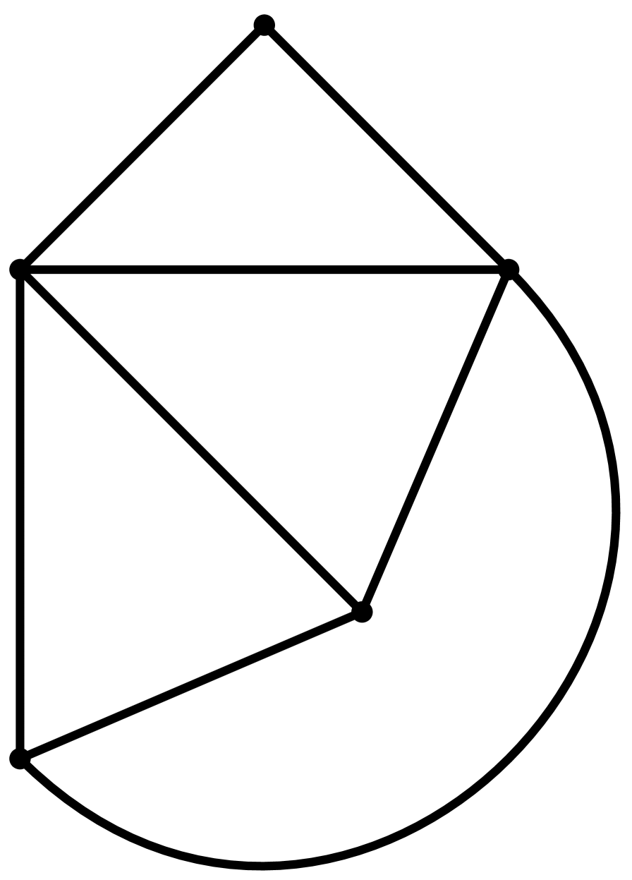
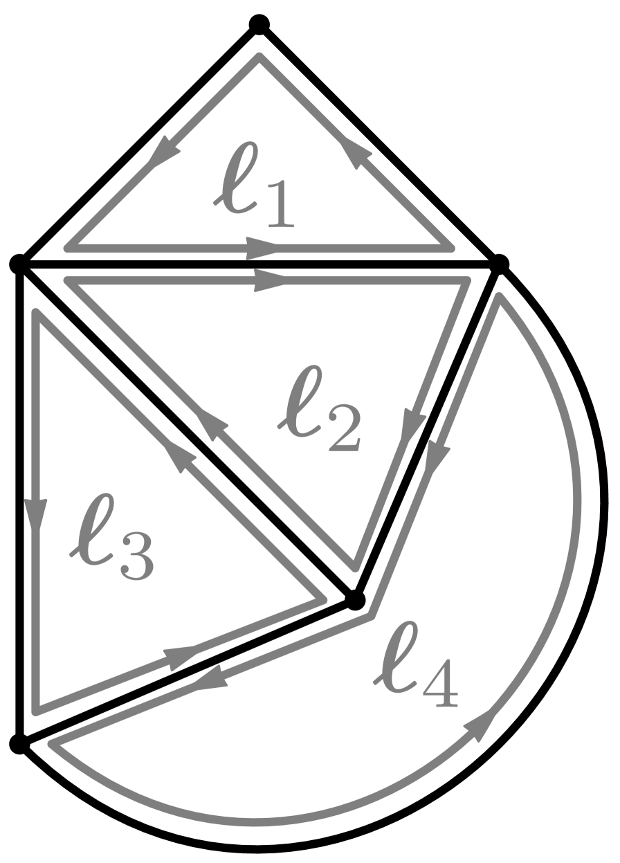
• (a)	(b)	(c)
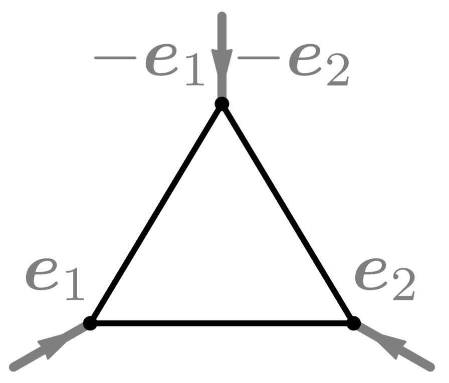
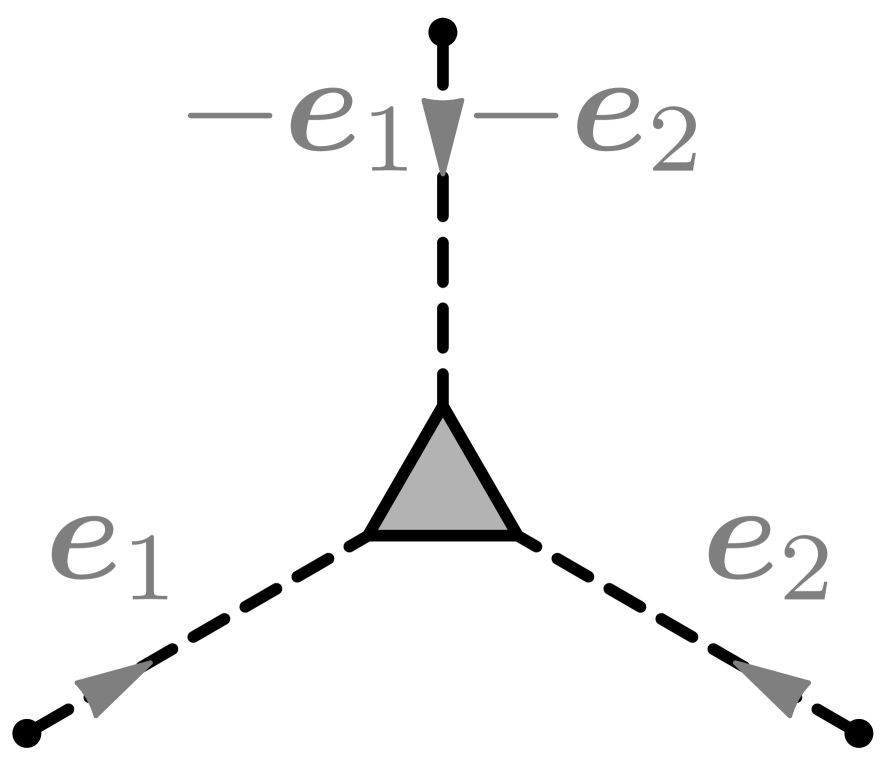
  (d)	(e)	(f)
  (g)	(h)	(i)

Figure 5: Parameterization of a four-loop diagram in terms of “triangles” [diagrams (a), (b) and (c)], and various steps in the parameterization of the diagram in Fig. 5(a) in terms of effective triangle vertices [diagrams (d)–(i)]. Further explanations are given in the text.

The diagram in Fig. 5(a) has four loops. After redrawing it as in Fig. 5(b) to highlight its planar structure, and assigning loop momenta as in Fig. 5(c), we can make use of standard Feynman rules for scalar theories in $3$ dimensions, arriving at the formula

$$\mathcal{A}\propto\int{\rm d}^{3}\bm{\ell}_{1}\,{\rm d}^{3}\bm{\ell}_{2}\,{\rm d}^{3}\bm{\ell}_{3}\,{\rm d}^{3}\bm{\ell}_{4}\, \;\mathrm{Pr}^{2}\!\left(\bm{\ell}_{1}\right)\;\mathrm{Pr}\!\left(\bm{\ell}_{3}\right)\;\mathrm{Pr}\!\left(\bm{\ell}_{4}\right)$$ (297)

$$\times\;\mathrm{Pr}\!\left(\bm{\ell}_{1}+\bm{\ell}_{2}\right)\;\mathrm{Pr}\!\left(\bm{\ell}_{2}+\bm{\ell}_{3}\right)\;\mathrm{Pr}\!\left(\bm{\ell}_{2}+\bm{\ell}_{4}\right)\;\mathrm{Pr}\!\left(\bm{\ell}_{3}-\bm{\ell}_{4}\right)\,,$$

which expresses the amplitude at zero external momenta (as specified by the renormalization scheme adopted in [281] and [274]) in terms of an integral representation of dimensionality $12$. The propagator $\mathrm{Pr}\!\left(\bm{\ell}\right)$ here is the scalar Euclidean kernel

$$\mathrm{Pr}\!\left(\bm{\ell}\right)=\frac{1}{\ell^{2}+m^{2}}\,.$$ (298)

The renormalized mass $m$ is set to one by the renormalization schemes used in [281] and [274]. Needless to say, starting from Eq. (297), it would be extremely difficult, if not impossible, to give a precise numerical estimate for the amplitude corresponding to the diagram in Fig. 5(a).

Now, we can formulate a much more efficient strategy to evaluate the diagram in Fig. 5(a), if we suppose for example to know, with its complete dependence on external momenta ${\bm{e}}_{1}$ and ${\bm{e}}_{2}$, the analytic formula for the one-loop $3$-dimensional integral corresponding to the “triangle” diagram of Fig. 5(d), that is,

$$\mathrm{Tri}\!\left({\bm{e}}_{1},{\bm{e}}_{2}\right)\equiv\int d^{3}\bm{\ell}\;\;\mathrm{Pr}\!\left(\bm{\ell}\right)\;\mathrm{Pr}\!\left(\bm{\ell}+{\bm{e}}_{1}\right)\;\mathrm{Pr}\!\left(\bm{\ell}+{\bm{e}}_{1}+{\bm{e}}_{2}\right)\,.$$ (299)

In fact, in this case we can identify in the right-hand side of Eq. (297) suitable subintegrals being of the form of the right-hand side of Eq. (299), replacing them with the analytic formula for the function $\mathrm{Tri}$; this operation can even be performed diagrammatically, by systematically substituting all occurrences of Fig. 5(d) with the “effective vertex” of Fig. 5(e), where the dashed lines attached to triangle vertices are used to automatically implement momentum conservation.

This method leads, after the simple graphical manipulations of Figs. 5(g), (h) and the choice of momenta of Fig. 5(i), to the new integral representation

$$\mathcal{A}\propto\int{\rm d}^{3}\bm{\ell}_{1}\;{\rm d}^{3}\bm{\ell}_{2}\;\;\mathrm{Tri}\!\left(\bm{\ell}_{1},-\bm{\ell}_{1}\right)\;\mathrm{Tri}\!\left(\bm{\ell}_{1},\bm{\ell}_{2}\right)\;\mathrm{Pr}\!\left(\bm{\ell}_{1}+\bm{\ell}_{2}\right)\;\mathrm{Pr}\!\left(\bm{\ell}_{2}\right)\,.$$ (300)

After the explicit parameterization of momentum space ${\rm d}^{3}\bm{\ell}_{1}\;{\rm d}^{3}\bm{\ell}_{2}$, this representation turns out to have a dimensionality of “only” $3$. In Ref. [273] a value of $0.1120344277(1)$ is quoted for this diagram (we notice that a suitable normalization factor therein described must be inserted into Eq. (300) to obtain this numerical result.)

As the four-loop diagram in Fig. 5(a) constitutes a relatively simple example, we would like to add that much more complex effective vertices than the triangle alone must be used to make this technique effective for the large sets of diagrams which are needed in the six- and seven-loop orders. In addition, the way of replacing effective vertices is not unique, possibly leading to many different integral representations, each one with a different final dimensionality. For example, as Fig. 5(f) already suggests, many other triangles than the two highlighted ones could be identified at different positions in the diagram (however, it should also be noticed that in this example the maximal number of triangles which can be replaced at the same time is always two, no matter which choice of triangles is considered). The identification of the most favorable parameterization defines a very complicated optimization problem, which, if connected to the very large number of diagrams to be evaluated, calls in turn for an automated way of finding out the most favorable parameterizations. A strategy to solve this problem in a more general and detailed way, even considering other possible analytic simplifications, is described in [296].

It should be noticed that in this approach the renormalization procedure can be built into the step of amplitude parameterization. The reason is that the $O\left(N\right)$ vector model is superrenormalizable in $3$ dimensions (see [296] for further details).

(iii) Numerical evaluation of the needed amplitudes. Each integral representation obtained during the last stage must be numerically evaluated at zero external momenta, following the renormalization-scheme prescriptions originally formulated in Ref. [281]. When combined with the symmetry factors and the $O\left(N\right)$ factors, as described above, this operation leads to the perturbative knowledge (up to the desired loop order) of RG functions $\beta$, $\eta$ and $\eta_{2}$ appearing in Eq. (295).

As previously emphasized, the difficulty implied by this stage should not be underestimated. For example, no published algorithm for multidimensional numerical integration is able to guarantee that the needed number of significant digits ($7$–$8$) will be obtained after a reasonable number of function evaluations for all needed $9$-dimensional integral representations at the level of $7$ perturbative loops. However, an innovative algorithm described in [297], which has been recently designed with this problem in mind, should finally allow to obtain an asymptotic behaviour of the integration error nice enough to reach the high precision required for this multi-dimensional computation.

(iv) Resummation of the obtained series. In order to complete the analysis of the critical exponents, we recall that the non-trivial value of the coupling $u$ such that the RG $\beta$-function in Eq. (294a) goes to zero must be identified numerically (this corresponds to the so-called Wilson-Fisher fixed point of the $O\left(N\right)$ vector model). One can then extract, for example, the value for the critical exponent $\alpha$ from the following formulas

$$\beta\!\left(u^{*}\right) = 0\,,$$ (301a)

$$\alpha = 2-\frac{d}{2-\eta\!\left(u^{*}\right)+\eta_{2}\!\left(u^{*}\right)}\,.$$ (301b)

In this physical situation, the critical value of the coupling is non-perturbatively large (we have $g^{*}\approx 1.4$ here), and therefore a suitable resummation of the series for the scaling functions is required to get meaningful results for the desired physical quantities. In addition, and as mentioned before, the mathematical property of Borel summability has been rigorously established in [293] for the $\left(\phi^{2}\right)^{2}$ theory in the case $d=3$, so applying the procedure of Borel resummation to this physical problem is definitely legitimate.

From an historical perspective, it is noteworthy that the first precise numerical evaluation of critical quantities has been derived in [274] by means of a Borel–Padé summation as described in Sec. 3.2.3. However, a spectacular theoretical breakthrough was achieved in the seminal paper [298, 176] when some additional information, derived from the large-order behavior analysis of perturbation theory for scalar quantum field theories carried out in [299], has been conveyed to the Borel resummation of these series (a detailed review of the subject with additional results can also be found in [300]). Such analysis states that the coefficients of the perturbative series for any critical quantity $S(g)$ behave at large perturbative orders $n$ as

$$S_{n}=c(-a)^{n}n^{b}n!\left(1-O\left(\frac{1}{n}\right)\right),$$ (302)

with $a$, $b$ and $c$ being computable numbers which depend on the critical function to be evaluated. In particular, $a$ turns out to be independent of the series under consideration and equal to

$$a=0.147774232(1)\frac{9}{N+8}$$

for the case $d=3$. It should be noticed how this discovery legitimates a posteriori the use of the Borel–Padé summation in [274], which had been proposed in that context as a mere guess.

If we introduce a generalized Borel-Leroy transform $B_{S}^{(1,b^{\prime})}(u)$ of $S(g)$, defined as

$$B_{S}^{(1,b^{\prime})}(u)=\sum_{n=0}^{\infty}\frac{S_{n}}{\Gamma\left(n+b^{\prime}+1\right)}u^{n},$$ (303)

(which differs from the formulas presented in Sec. 3.2.1 only for the presence of an arbitrary parameter $b^{\prime}$), Eq. (302) shows that the closest singularity of $B_{S}^{(1,b^{\prime})}(u)$ (called instanton singularity) is located at the point $-1/a$ (we refer the reader to [177] for a more detailed discussion about both this fact and the used terminology).

If the additional hypothesis is formulated that all the finite-distance singularities of the Borel transform of the series come from subleading instantonic contributions (which are located further away on the negative axis of the complex plane), and the Borel transform is thus supposed to be analytic in the whole complex plane except for the cut going from $-1/a$ to $-\infty$ (this statement is also known as the maximal analyticity hypothesis), then a conformal mapping specially tailored to the analytic structure of the series can be used, leading to a remarkable enhancement in the accuracy of the obtained resummed quantities. It should be noticed that, contrary to the property of Borel summability, the property of maximal analyticity has not been rigorously proven for the case of $d=3$; however, arguments for its plausibility are given in [177].

We then arrive again at a method based on the conformal mapping of the Borel plane, which we have already discussed in detail in Sec. 3.2.4: by introducing the transformation

$$z\left(u\right)=\frac{\sqrt{1+au}-1}{\sqrt{1+au}+1}\,,$$ (304)

we map the Borel plane, cut at the instanton singularity $u=-1/a$, onto a circle in the $z$ plane in such a way to enforce maximal analyticity, and thus to enhance the rate of convergence. With the help of Eq. (304), we can now rewrite the Borel transform (303) upon expansion of the $u$ in powers of $z$:

$$B^{(1,b^{\prime})}_{S}\left(u(z)\right)=\sum_{n=0}^{\infty}\ s^{[b^{\prime}]}_{n}\,z^{n}\,.$$ (305)

where the coefficients $s^{[b^{\prime}]}_{n}$ can be uniquely determined as function of $S_{n}$. Finally, the full physical solution $S(g)$ can be reconstructed by evaluating the Laplace–Borel integral:

$$S\!\left(g\right) = \frac{1}{g^{b^{\prime}+1}}\,\int\limits_{0}^{\infty}u^{b^{\prime}}\exp(-u/g)\,B^{(1,b^{\prime})}_{S}\left(u(z)\right)\,{\rm d}u$$ (306)

$$= \frac{1}{g^{b^{\prime}+1}}\,\sum_{n=0}^{\infty}s^{(b^{\prime})}_{n}\int_{0}^{\infty}u^{b^{\prime}}\exp(-u/g)\left[z(u)\right]^{n}{\rm d}u\,.$$

Interestingly, it is possible to connect the so far arbitrary parameter $b^{\prime}$ to $b$, and use it as a variational check to validate the method; in addition, introducing more complicated prescriptions the knowledge of $c$ can be incorporated in the resummation algorithm as well (the reader interested in this point may wish to consult [176]). In this way, one can properly take advantage of all the available information about the analytical properties of the critical quantities. Finally, additional refinements of the method described here are possible, like considering an additional homographic transformation to displace possible complex singularities in the $g$-plane [254].

However, we would like to mention that many other resummation methods have been proposed and implemented in this context. For example, an alternative approach which does not make use neither of Borel summation nor of Padé approximant is that of order-dependent mapping given in [210] and [211]; to the best of our knowledge, this method too has been invented for the particular case of the resummation of critical exponents.

Anyway, let alone the problem of finding the correct value for the resummed series, we would like to emphasize how an even greater care should be spent in giving an accurate evaluation of the final uncertainty of the resummation. In fact, the error in critical quantities basically comes from two sources, the summation error at fixed $g^{\ast}$, $\Delta S$, and the error induced by the error in $g^{\ast}$, $\Delta\tilde{g}^{\ast}$:

$$S=S^{\ast}\pm\Delta S\pm\left(\frac{dS}{d\tilde{g}}\right)_{\tilde{g}^{\ast}}\Delta\tilde{g}^{\ast}.$$ (307)

In this respect, the computation of some auxiliary quantities like the shifted series

$$S_{s}\left(z\right)=\frac{1}{z^{s}}\left(S\left(z\right)-\sum_{k=0}^{s-1}S_{k}z^{k}\right),s\in{1,2},$$ (308)

or the series $1/S$, can give precious hints about the spread of the numerical results, thus ultimately leading to a reasonable indication about the summation errors. A sophisticated analysis of the error bounds, as well as a careful review of the values for critical quantities obtained by Borel resummation from quantum field theoretical techniques can be found in [254] (see also the earlier work [298]).

3.7.4 Concluding Remarks on Renormalization Group–Related Quantities

Since the determination of critical exponents is a particularly prominent application of numerical convergence “accelerators” and summation techniques for divergent series, we would like to include here a few remarks regarding possible foreseeable progress in this field. Indeed, there is some hope that the computations presented in the two last subsections can be partly extended in a not too distant future.

As discussed in [301], in the case of the HT series the main computational problem is apparently a graph-theoretical one. In particular, the algorithm of generation of the set of graph required for the LCE is very inefficient, being plagued by the so-called problem of isomorphic copies: every known algorithm for graph enumeration generates some subset of the needed graphs more than once, so that the effective number of graphs to be scanned during the generation stage can be orders of magnitude larger than the dimension of the desired final set. In addition, storage problems are quite common during the computation of the series (see Refs. [259, 260, 261]). As a matter of fact, the reached level of $20$-$25$ terms of HT series seems to be close to the saturation of presently available computational resources.

Similar considerations can be carried out in the case of the approach at fixed dimension: even if promising steps have been done in [296] towards the full extension to $7$ perturbative loops of the original $6$-loop computation of [274], the method does not appear to be easily extensible to a higher perturbative level. The most relevant problem with such an approach lies in the fact that there is no a priori proof of its validity: no theorem exists stating that at a given loop order, for a given set of available effective vertices, some minimal reduction in the number of residual integrations will be obtained uniformly for all graphs needed for the evaluation of the desired physical quantities; the effectiveness of the method can in fact be demonstrated only a posteriori, by an explicit inspection carried out diagram by diagram. Indeed, such a proof has been recently given in [296] for the level of $7$ perturbative loops; however, it is unlikely that the method can be extended much further, since each loop more raises the upper bound for the dimensionality of the residual integration which must be carried out for each Feynman diagram, thus quickly making things computationally too expensive even if the considered set of effective vertices is quite large.

Other computational schemes for RG quantities which are less suffering from this explosive growth in computational complexity with the order of the approximation do exist — notably Monte-Carlo methods. As mentioned before, it is possible with these methods to reach a precision comparable to that of the experimental results so far available; however, also the scaling of these algorithms is actually very bad, requiring as well a formidable consumption of computational resources (for example, the sophisticated theoretical estimates quoted in [251] required about $20$ years of total CPU time).

In any case, while some progress can certainly be achieved with all three of the above mentioned methods, it appears unlikely that any of the theoretical techniques known so far will be able to reach a precision comparable to that foreseen for the next generation of experiments (which should be at least one order of magnitude better than the accuracy reached so far). Perhaps some theoretical breakthrough could change this picture.

4 Conclusions

First, let us give a synopsis of the convergence acceleration methods discussed in Sec. 2 of this review. We can summarize a few important aspects as follows:

1. As has been emphasized in [31] and here, our theoretical knowledge of the properties of many of the algorithms is incomplete, although an important classification can be given in terms of alternating and nonalternating, as well as linearly and logarithmically convergent series. We can say that a theory of their properties, if it is to be considered as satisfactory from a practical point of view, should provide a theoretical estimate of the numerical stability properties in addition to the convergence acceleration properties of the transforms.

2. None of the convergence accelerators discussed here is linear in the sense that the $n$th-order transform of the sum of two input series is equal to the sum of the $n$th-order transforms of the two input series. Linearity is thus not provided. However, a weaker requirement called translation under translation can in general be imposed [see, e.g., Eq. (3.1-4) of Ref. [31]]. It is generally acknowledged nowadays that the nonlinear transformations discussed in this review potentially lead to much better numerical results that typical linear convergence acceleration schemes.

3. Logarithmically convergent sequences are rather difficult to accelerate; in particular, they constitute a set with the property of remanence (see Ref. [25]), thus satisfying the hypothesis of a “non-universality” theorem [79]. This implies that no universal sequence transformation exists which is able to accelerate all the sequences belonging to the set; in other words, a given method will work only for some subset of the logarithmic sequences, and will not work for all the others. However, a few potentially very powerful algorithms can be indicated (see, e.g., Sec. 2.2.2 and Table 1).

4. It would be a hopeless task to attempt an exhaustive overview of all available convergence acceleration methods in this review. As an example of an algorithm which is not discussed here, we only mention the Overholt process and the ACCES algorithms which are described in detail in Ref. [25], or the Euler transformation and the Euler–Maclaurin formula which are discussed in many standard reference books on mathematical methods for the physics community (e.g., Ref.[161, 76]). We have only attempted to provide a general overview of some available methods, to introduce a rather universally applicable construction principle via the $E$-algorithm (see Sec. 2.2.7), and to illustrate these general concepts by considering some examples. The interested reader will find further information in the more specialized literature indicated in Sec. 2.

5. If one is simply interested in numerical results, there may be a strong motivation to skip the theoretical phase of the algorithm-finding process sketched in Sec. 2 to a large extent, and to investigate the performance of convergence accelerators experimentally. It is undeniable that this approach if far from satisfactory from a theoretical point of view, but it can lead, nevertheless, to numerically spectacular results. In the case of no available analytic information, experiments are even unavoidable. In this context, one might note that according to Refs. [106, 302], the nonlinear sequence transformation listed in Table 1, notably the $d$ and $\delta$ transformations discussed in Sec. 2.2.3 below, are among the most powerful and most versatile sequence transformations for alternating series that are currently known.

6. The notion of a certain “complementarity” appears to be rather universally applicable to the field of convergence acceleration algorithms, in various contexts. E.g., the $\epsilon$ algorithm is known to be an efficient accelerator for linearly convergent and even factorially divergent input series, but fails for logarithmically convergent input data. The $\rho$ algorithm is known to be an efficient accelerator for logarithmically convergent input series, but fails for linearly convergent and factorially divergent input data. Both the $\epsilon$ and $\rho$ algorithms are numerically rather stable and rather universally applicable to series in their respective domains, but are in many cases outperformed by special sequence transformations which profit from explicit remainder estimates. On the other hand, the sequence transformation with remainder fails completely if the assumptions about the structure of the remainder term are not met by a given input series.

7. The notion of “complementarity” also affects the “iteratability” of the transformations: Relatively simple sequence transformations like the $\Delta^{2}$ process, which make only very crude assumptions about the structure of the remainder term, can typically be iterated, leading to improvements in higher orders of the iteration process. In sharp contrast, the elimination of a complex remainder structure as implied by a sequence transformation with a remainder estimate intuitively leads to the conjecture that a further iteration of the process cannot increase the apparent convergence any further. This is indeed confirmed in numerical studies performed by the authors, and illustrates the general complementarity aspect of the convergence accelerators once more: the power of a specialized algorithm has to be traded for a disadvantage in the sense that further iterations typically cannot increase the numerical gain of a single iteration.

The perhaps most important application of the convergence acceleration techniques is the calculation of the hydrogen Green function, described in Sec. 2.4.2. Namely, while the so-called $Z\alpha$-expansion (“perturbative bound-state QED”) in general converges better for low nuclear charges $Z$ than for high $Z$, it is necessary, at the current level of accuracy, to even include nonperturbative effects at low $Z$. This surprising observation is especially important for the one-loop self-energy correction, which is the dominant radiative correction in hydrogenlike ions. To give an example, the difference between all known terms of the $Z\alpha$-expansion up to the order $\alpha(Z\alpha)^{6}mc^{2}$ (Ref. [303]) and the nonperturbative, higher-order remainder for the 1S state [35] amounts to $28\,{\rm kHz}$. This is about 700 times larger than the current best measurement in atomic hydrogen, which has an accuracy of about $40\,{\rm Hz}$ [304, 305]. Thus, while corrections of smaller absolute magnitude can still be described perturbatively at low $Z$ (e.g., two-photon effects), the dominant one-photon corrections have to be calculated nonperturbatively to match current experimental precision, and from this point of view, atomic hydrogen ($Z=1$) constitutes a “high-Z system” whose description would be incomplete without a calculation of the nonperturbative effects. An essential ingredient in that direction is given by the methods discussed in Sec. 2.4.2.

Regarding divergent series and Borel summation treated in Sec. 3, one important conclusion is that even the best summation method cannot reconstruct a complete physical answer from perturbation theory alone, if there are instanton-related contributions, nonperturbatively suppressed, which must be added to the perturbative expansion. This has been seen in one-dimensional model problems, notably in the case of double-well like potentials treated in Sec. 3.6. In the calculation [248], an attempt has been made to use resurgent expansions at moderate and large couplings, for a few nontrivial cases of one-dimensional potentials which, nevertheless, admit a treatment via generalized quantization conditions. The conclusion has been that while the resurgent expansion can be useful to explore nonperturbative effects at small coupling, it cannot be used for accurate quantitative methods in the asymptotic strong-coupling region. Roughly speaking, the triple resummation of the resurgent series in $n$, $k$ and $l$ in Eq. (273) is too hard for any available summation algorithms to handle even if one enters directly into the quantization condition (270) and directly resums the $A_{\rm dw}$ and $B_{\rm dw}$ function given in Eqs. (271) and (272). Nevertheless, the accurate understanding of nonperturbative effects in quantum potentials with instanton contributions via resurgent expansions at small and moderate coupling could be seen as a significant consequence of the understanding gained by the path integral formalism. Let us also mention that important connections of the quantum oscillators to field theoretical problems exist, as explained in detail in Ref. [177].

We should perhaps mention that our treatment of the even and odd anharmonic oscillators in Secs. 3.4 and 3.5 is entirely based on the concept of distributional Borel summation and thus far from exhaustive. One aspect left out in this review concerns renormalized strong coupling expansions [306, 307] and related methods (see also [308, 102, 108, 309, 310, 112, 307, 111]) which make possible the determination of very accurate numerical energy eigenvalues using only few perturbative coefficients, and which cover both small and large couplings. Expansions of this kind, however, fail for double-well like potentials and also cannot reproduce the width of resonances in the case of an odd perturbation.

To conclude this review, let us indicate some open problems and directions for further research. (i) There is a regrettable absence of a general mathematical proof for the convergence of some of the nonlinear sequence transformations described in Sec. 2. This might lead to a direction of research for mathematics. Only for some special model problems could rigorous convergence proofs be obtained (see [311, 312, 313] or Sections 13 and 14 of [31]). (ii) New sequence transformations with improved remainder estimates could be a significant direction of research for both physics and mathematics. In this context, one might mention hyperasymptotics (see Ref. [76] and a couple of preparatory calculations, e.g., Refs. [314, 315]. (iii) For nonalternating divergent series, the next term omitted from the partial sum of the asymptotic series is typically not a good simple remainder estimate. One may indicate the unsolved problem of finding a practically useful remainder estimates for nonalternating divergent series, in particular those which give rise to an imaginary part in the sense of a distributional Borel summation. (iv) Let us also indicate a possibly interesting further direction in the field-theoretical direction which is based on the following observation: In general, a perturbation potential or a field interaction determines the large-order behaviour of the generated perturbation series. However, the interaction potential also determines the large-coupling expansion of the related quantities. This means that there should be a connection between the large-coupling expansion and the large-order behaviour of the perturbation series. This notion and related ideas about connections of weak- and strong-coupling regimes have quite recently been explored in Refs. [316, 317, 255, 66, 67, 68, 69], but further work in this direction is definitely needed. (v) Finally, there is a possible connection of the “prediction” or extrapolation of perturbative coefficients as described here in Sec. 2.2.5, and Brodsky–Lepage–Mackenzie (BLM) scale setting [318] which is based on the idea that, roughly speaking, seemingly wildly divergent perturbative expansions in field theory can sometimes be formulated as not so wildly divergent series if the expansion variable (coupling constant) is taken at a momentum scale appropriate to the problem. This approach is illustrated in Ref. [318] using the two-loop correction to the muon anomalous magnetic as an example, and a related approach has recently been generalized to higher orders in Ref. [319]. However, it seems that there is still room for improvement in the renormalization-group-inspired approaches to the extrapolation of perturbative expansions to higher-order loop corrections in field theory.

Acknowledgements

First and foremost, the authors would like to acknowledge elucidating and insightful discussion with Professor Ernst Joachim Weniger. His seminal contributions to the field have been a significant motivation and inspiration to write the current review. In addition, the authors acknowledge helpful discussions with Sergej V. Aksenov, Jens Becher, and Professor Sandro Graffi as well as Professor Jean Zinn–Justin. P.R. acknowledges the stimulating atmosphere at Gesellschaft für Schwerionenforschung (GSI). U.D.J. acknowledges support by the Deutsche Forschungsgemeinschaft (Heisenberg program). Finally, we would include an apology for the necessarily incomplete list of references of this review; and this goes out to all the authors whose work we failed to cite here.

Appendix A Basic Terminology for the Spectra of Hamilton Operators

A.1 Resolvent, Spectrum, Green’s Function

In this subsection we shortly recall, for the convenience of the reader, some of the basic mathematical definitions concerning spectral theory of Schrödinger operators, including resonances. A standard reference for these topics is [44].

Definition 16

Given a closed operator $H$ in a Hilbert space ${\cal H}$ with domain $D(H)$, its resolvent set $\rho(H)$ is the set of all $\lambda\in{\mathbbm{C}}$ such that the operator $H-\lambda I$ (where $I$ is the identity operator) is invertible and its range $R(H-\lambda I)$ is the whole of ${\cal H}$.

By the closed graph theorem (see e.g. [320], Theorem III.5.20) the inverse operator $R(\lambda,H)=(H-\lambda I)^{-1}$, which by the above definition exists and has domain ${\cal H}$, is bounded, or, equivalently, continuous, namely there is $C(\lambda)>0$ such that, for all $u\in{\cal H}$:

$$\|R(\lambda,H)u\|\leq C(\lambda)\|u\|\,.$$ (309)

$\rho(H)$ is called resolvent set because the linear inhomogeneous equation $(H-\lambda I)u=f$ in the unknown $u\in{\cal H}$ can always be solved: it has indeed the unique solution $\displaystyle u=R(\lambda,H)f$ for any datum $f\in{\cal H}$ if $\lambda\in\rho(H)$.

Definition 17

The complement of $\rho(H)$ with respect to ${\mathbbm{C}}$, i.e. the set of all $\lambda\in{\mathbbm{C}}$ such that either $R(\lambda,H)$ does not exist (in the sense that the operator $H-\lambda I$ is not invertible), or, if it does, its domain is not ${\cal H}$, is the spectrum of $H$, denoted $\sigma(H)$.

The following examples can be given:

1. Let $H$ be a $n\times n$ matrix acting on ${\cal H}={\mathbbm{C}}^{n}$. Its spectrum $\sigma(H)$ is clearly the set of the eigenvalues of $H$, because $H-\lambda I$ is not invertible if and only if $Hu=\lambda u$ for some $u\neq 0$, i.e. ${\rm det}(H-\lambda I)=0$. On the other hand, if $H-\lambda I$ is invertible, its range is always ${\cal H}$ because ${\cal H}$ has finite dimension.

2. Likewise, in general any eigenvalue $E$ of $H$ belongs to $\sigma(H)$, because for any corresponding eigenvector $\psi$ one has $(H-EI)\psi=0$. Therefore the spectrum always contains the eigenvalues.

3. If the Hilbert space is infinite dimensional, however, the spectrum may have a totally different nature. Let for instance $H=X$ be the position operator in quantum mechanics, namely the maximal multiplication operator by $x$ in $L^{2}({\mathbbm{R}})$. Its action and domain are:

   $$(Xu)(x)=xu(x)\,,\qquad D(X)=\left\{u\in L^{2}({\mathbbm{R}}):xu(x)\in L^{2}({\mathbbm{R}})\right\}=$$

   $$\left\{u(x):\int_{{\mathbbm{R}}}|u(x)|^{2}\,{\rm d}x<+\infty;\int_{{\mathbbm{R}}}|xu(x)|^{2}\,{\rm d}x<+\infty\right\}\,.$$ (310)

   Then $\sigma(X)={\mathbbm{R}}$. We obviously have, indeed:

   $$((R(\lambda,X)u)(x)=\frac{u(x)}{x-\lambda}\,.$$ (311)

   Now, for any given $\lambda\in{\mathbbm{R}}$, pick $u(x)\in L^{2}({\mathbbm{R}})$ continuous and nonzero in an open interval around $\lambda$. Then $\int_{{\mathbbm{R}}}\frac{|u(x)|^{2}}{|x-\lambda|^{2}}\,{\rm d}x$ does not exist and hence $R(X,\lambda)$ is not defined on the whole of ${\cal H}$.

The most important example in the present context is represented by the Schrödinger operator $H=T+V$ acting in $L^{2}({\mathbbm{R}}^{n})$. Here $T$ is the kinetic energy operator, and $V$ the (real-valued) potential. In units with $\hbar=1$, these read

$$(Tu)(x)=-\Delta u(x)\,,\quad u\in D(T)\,,\qquad(Vu)(x)=V(x)u(x)\,,\quad u\in D(V)\,.$$ (312)

Here, $D(T)$ and $D(V)$ are the maximal domains of $T$ and $V$, namely

$$D(T)=\{u\in L^{2}({\mathbbm{R}}^{n}):\Delta u\in L^{2}({\mathbbm{R}}^{n})\},\qquad D(V)=\{u\in L^{2}({\mathbbm{R}}^{n}):Vu\in L^{2}({\mathbbm{R}}^{n})\}\,.$$ (313)

We take as the domain $D(H)$ the maximal one,

$$D(H)=\{u\in L^{2}({\mathbbm{R}}^{n}):-\Delta u+Vu\in L^{2}({\mathbbm{R}}^{n})\}\,.$$ (314)

It is easy to see that $T$ and $V$ are self-adjoint operators, namely $T=T^{\ast}$, $V=V^{\ast}$, where $A^{\ast}$ denotes the adjoint of the operator $A$. Under suitable conditions on $V$ (see Ref. [44], Chap. 10), also $H$ is self-adjoint (with the proof being often far from trivial). Concerning self-adjointness, we recall that:

1. If $A$ is any self-adjoint operator in ${\cal H}$, then $\sigma(A)\subset{\mathbbm{R}}$.

2. The symmetry property $\langle Au|v\rangle=\langle u|Av\rangle$, $\forall\,(u,v)\in D(A)$ is not sufficient to guarantee self-adjointness because it implies only $A^{\ast}u=Au$ for $u\in D(A)$ but it does not exclude $D(A)\neq D(A^{\ast})$. The difference is quite substantial because while the spectrum of a self-adjoint operator is real, the spectrum of a symmetric but not self-adjoint operator is the whole of ${\mathbbm{C}}$.

By its very nature, any Schrödinger operator is a differential operator acting on a Hilbert space of functions. This makes it possible to characterize its resolvent and spectrum in terms of the solutions of the time-independent Schrödinger equation $(-\Delta+V)\,\psi=E\,\psi$.

Definition 18

For any $\lambda\in{\mathbbm{C}}$, let ${\cal G}(x;\lambda)$ be a distributional solution of the inhomogeneous equation

$$-\Delta{\cal G}(x;\lambda)+[V(x)-\lambda]{\cal G}(x;\lambda)=\delta(x),\quad x\in{\mathbbm{R}}^{n}\,,$$ (315)

with $\delta(x)$ being the Dirac distribution. Under very general conditions on $V$, it can be proven that ${\cal G}(x;\lambda)$ is unique, and it is called fundamental solution, or Green function, of the Schrödinger operator $H=T+V$.

The Green function yields an explicit representation of the resolvent $[H-\lambda I]^{-1}$. Consider indeed the integral operator in $L^{2}({\mathbbm{R}}^{n})$ of kernel ${\cal G}(x-y;\lambda)$, namely the operator acting on functions $u\in L^{2}$ in the following way:

$$(G(\lambda)\,u)(x)=\int_{{\mathbbm{R}}^{n}}{\cal G}(x-y;\lambda)\,u(y)\,{\rm d}y\,.$$ (316)

We have, for any $u\in L^{2}$ (the interchange between differentiation and integration can be justified):

$$(H-\lambda\,I)(G(\lambda)\,u)(x)=[-\Delta+V(x)-\lambda]\,\int_{{\mathbbm{R}}^{n}}{\cal G}(x-y;\lambda)\,u(y)\,{\rm d}y=$$ (317)

$$=\int_{{\mathbbm{R}}^{n}}[-\Delta+V(x)-\lambda]\,{\cal G}(x-y;\lambda)\,u(y)\,{\rm d}y=\int_{{\mathbbm{R}}^{n}}\delta(x-y)\,u(y)\,{\rm d}y=u(x)\,.$$ (318)

This shows that $G(\lambda)$ is the inverse of $[H-\lambda I]$, and therefore coincides with the resolvent operator. Hence the above formula yields the explicit action of the resolvent $R(\lambda,H)$:

$$R(\lambda,H)\,u(x)=\int_{{\mathbbm{R}}^{n}}{\cal G}(x-y;\lambda)\,u(y)\,{\rm d}y\,.$$ (319)

As an example, consider the free particle energy operator in one dimension,

$$H=T=-\frac{{\rm d}^{2}}{{\rm d}x^{2}},\qquad D(T)=\{u:u\in L^{2},u^{\prime}\in L^{2},u^{\prime\prime}\in L^{2}\}\,.$$ (320)

The differential equation for the Green function is therefore

$$-{\cal G}^{\prime\prime}(x;\lambda)-\lambda\,{\cal G}(x;\lambda)=\delta(x)\,.$$ (321)

To solve this equation, we switch to Fourier space. Let $\hat{{\cal G}}(p;\lambda)$ be the Fourier transform of ${\cal G}(x;\lambda)$:

$$\hat{{\cal G}}(p;\lambda)=\frac{1}{\sqrt{2\pi}}\,\int_{\mathbbm{R}}{\cal G}(x;\lambda)\,{\rm e}^{-{\rm i}px}\,{\rm d}x\,.$$ (322)

Then (integrating twice by parts) we have

$$\frac{1}{\sqrt{2\pi}}\int_{\mathbbm{R}}{\cal G}"(x;\lambda)\,{\rm e}^{-{\rm i}px}\,{\rm d}x=p^{2}\hat{{\cal G}}(p;\lambda)\,.$$ (323)

Since $\int_{\mathbbm{R}}\delta(x){\rm e}^{-{\rm i}px}\,{\rm d}x=1$, the differential equation becomes

$$[p^{2}-\lambda]\hat{{\cal G}}(p;\lambda)=\frac{1}{\sqrt{2\pi}}\quad\Longrightarrow\quad\hat{{\cal G}}(p;\lambda)=\frac{1}{\sqrt{2\pi}(p^{2}-\lambda)}\,.$$ (324)

If we now invert the Fourier transform (using for instance complex integration) we readily obtain

$${\cal G}(x;\lambda)={\rm e}^{\sqrt{-\lambda}\,|x|}\,.$$ (325)

Hence, we have

$$R(T,\lambda)u=[T-\lambda I]^{-1}\,u(x)=\int_{{\mathbbm{R}}}{\rm e}^{\sqrt{-\lambda}\,|x-y|}\,u(y)\,{\rm d}y\,.$$ (326)

From this representation, we immediately see that $\sigma(T)=[0,+\infty)$ as it should be. If indeed $\lambda\in{\mathbbm{C}},\lambda\notin{\mathbbm{R}}_{+}$, then we have for all $u\in L^{2}$, with $\lambda=|\lambda|\,\exp({\rm i}\phi)$:

$$\|R(T,\lambda)u\|^{2}\leq\int_{\mathbbm{R}}\int_{\mathbbm{R}}|{\rm e}^{2\sqrt{-\lambda}\,(x-y)}|\,|u(y)|^{2}\,{\rm d}y\,{\rm d}x\leq\int_{\mathbbm{R}}|u(y)|^{2}\,{\rm d}y\,\int_{\mathbbm{R}}{\rm e}^{-2\sqrt{|\lambda|}\,\sin{(\phi/2)})\,|x-y|}\,{\rm d}x$$

$$\leq\frac{1}{\sqrt{|\lambda|}\,\sin{(\phi/2)}}\,\int_{\mathbbm{R}}|u(y)|^{2}\,{\rm d}y=C(\lambda)\,\|u\|^{2}\,,\qquad C(\lambda)=\frac{1}{\sqrt{|\lambda|}\sin{(\phi/2)}}\,,$$ (327)

whence the boundedness of $R(\lambda,T)$ because $0<C(\lambda)<+\infty$ as long as $0<\phi<2\pi$, i.e. $\lambda\notin[0,+\infty)$. In three dimensions with $x=(x_{1},x_{2},x_{3})$, in exactly the same way we obtain for the Green function of $T=-\Delta$:

$${\cal G}(x;\lambda)=\frac{{\rm e}^{\sqrt{-\lambda}\,\|x\|}}{\|x\|},\quad\|x\|=\sqrt{x_{1}^{2}+x_{2}^{2}+x_{3}^{2}}\,.$$ (328)

As above, we can check that $\sigma(T)=[0,+\infty)$.

In the above examples, the spectrum is continuous. The question emerges how to characterize the spectrum in terms of the solutions of the Schrödinger equation. We recall that by definition, $E$ is an eigenvalue of the Schrödinger operator $H$ (and hence a quantum bound state) if there is a non-zero function $\psi(x,E)\in L^{2}({\mathbbm{R}}^{n})$ (and hence normalizable: in other words, $\int_{{\mathbbm{R}}^{n}}|\psi(x,E)|^{2}\,{\rm d}x=1$) such that $H\psi=E\psi$. Then, $\psi(x,E)$ is called an eigenfunction corresponding to $E$. The number $m$ of linearly independent $L^{2}$ solutions of $H\psi=E\psi$ is the multiplicity of the eigenvalue $E$. By the normalization condition, all eigenfunctions corresponding to any bound state vanish as $\|x\|\to+\infty$. Hence $E$ is an eigenvalue of the Schrödinger operator if and only if the Schrödinger equation $H\psi=E\psi$ admits at least one normalizable solution. It is well known that eigenfunctions corresponding to different eigenvalues of a symmetric operator are orthogonal:

$$\langle\psi(x,E)|\psi(x,E^{\prime})\rangle=\int_{{\mathbbm{R}}^{n}}\psi(x,E)\,\overline{\psi}(x,E^{\prime})\,{\rm d}x=0,\quad E\neq E^{\prime}\,.$$ (329)

Linearly independent eigenfunctions corresponding to the same eigenvalue can always be chosen to be orthogonal by the Gram-Schmidt orthogonalization procedure when ${\cal H}$ is separable, i.e. when ${\cal H}$ contains a countable basis. It follows that the eigenfunctions corresponding to the bound states form an orthonormal system. If the spectrum consists entirely of eigenvalues, this system is complete, namely every vector in ${\cal H}$ can be expanded in Fourier series of the eigenvectors.

Under very general conditions on $V$, it can actually be proven that any eigenfunction is continuous and vanishes at least exponentially (pointwise), i.e. there is $K(E)>0$ such that

$$|\psi(x,E)|\leq{\rm e}^{-K(E)\|x\|},\quad\|x\|\to\infty\,.$$ (330)

The points belonging to the continuous spectrum of $H$ can be characterized in terms of the solutions of the stationary Schrödinger equation $H\psi=E\psi$ having a totally different behaviour at infinity:

A point $\lambda\in{\mathbbm{R}}$ belongs to the continuous spectrum of $H$ if and only if there is a solution $f(x,\lambda)\notin L^{2}$ of the Schrödinger equation $H\,f=\lambda\,f$ which fulfills the pointwise bound $|f(x,\lambda)|\leq K(\lambda)$ for some $K(\lambda)>0$ and all $x\in{\mathbbm{R}}^{n}$.

Again, it is useful to consider an example. Consider once again the kinetic energy $T$ in one dimension. Setting $\lambda=k^{2},k\in{\mathbbm{R}}$, the Schrödinger equation $T\psi=E\psi$ becomes

$$-\frac{d^{2}}{{\rm d}x^{2}}\psi(x,k)=k^{2}\psi(x,k)$$ (331)

with the well known plane wave solutions

$$\psi(x,k)={\rm e}^{\pm{\rm i}kx}\,,$$ (332)

which are not in $L^{2}$ because $|\psi(x,k)|=1$ if and only if $k\in{\mathbbm{R}}$; however $\psi(x,k)$ is obviously bounded if and only if $k\in{\mathbbm{R}}$, and hence $\lambda\geq 0$. The functions $\psi(x,k)$ are often called continuum eigenfunctions or sometimes generalized eigenfunctions. Since $\int_{\mathbbm{R}}{\rm e}^{{\rm i}kx}\,{\rm d}x=2\pi\delta(k)$, where $\delta(k)$ is the Dirac distribution, they fulfill the continuum orthogonality relations

$$\int_{\mathbbm{R}}\psi(x,k)\,\overline{\psi}(x,k^{\prime})\,{\rm d}x=\delta(k-k^{\prime})\,.$$ (333)

Sometimes, this relation is written under the form $\langle\psi(x,k)|\psi(x,k^{\prime})\rangle=\delta(k-k^{\prime})$ even if the scalar product in the right-hand side does not make sense because $\psi(x,k)\notin L^{2}$.

Solutions of the Schrödinger equation which are both non-normalizable and unbounded have no relation with the spectrum.

We recall that an orthonormal system (ON) in a (separable) Hilbert space ${\cal H}$ is a (finite or countable) set of vectors $\psi_{n}$, with $n\in\mathbbm{N}_{0}$, such that $\langle\psi_{n}|\psi_{m}\rangle=\delta_{m,n}$. Given any vector $u\in{\cal H}$, its Fourier coefficients with respect to the given ON system are by definition the scalar products

$$a_{n}=\langle u|\psi_{n}\rangle\,.$$ (334)

The ON system is complete when any vector in ${\cal H}$ can be expanded in Fourier series, namely when

$$u=\sum_{n=0}^{\infty}a_{n}\psi_{n}\,,$$ (335)

where the convergence takes place in the norm of ${\cal H}$.

If the spectrum of the Schrödinger operator $H$ is discrete, namely it contains only isolated eigenvalues of finite multiplicity, then the set of all its eigenfunctions can be selected in such a way that it forms a complete ON system. The same property holds in general for any self-adjoint operator with discrete spectrum.

Let us consider again some example. Let $H$ be the quantum harmonic oscillator, $H=-\frac{{\rm d}^{2}}{{\rm d}x^{2}}+x^{2}$ defined on its maximal domain. Then its spectrum is discrete, because it can be proven that it contains only the simple eigenvalues $E_{n}=2n+1$ with $n\in\mathbbm{N}_{0}$. The corresponding eigenfunctions are the Hermite functions $\psi_{n}(x)=\frac{1}{\sqrt{2^{n}\,n!\,\sqrt{\pi}}}\,{\rm e}^{-x^{2}}\,H_{n}(x)$, where $H_{n}(x)$ is the $n$th Hermite polynomial. The system $\psi_{n}$ is orthonormal and complete:

$$u(x)=\sum_{n=0}^{\infty}a_{n}\psi_{n}(x),\qquad a_{n}=\frac{1}{\sqrt{2^{n}\,n!\,\sqrt{\pi}}}\,\int_{\mathbbm{R}}u(x)\,{\rm e}^{-x^{2}}H_{n}(x)\,{\rm d}x\,.$$ (336)

The convergence takes place in the $L^{2}$ norm (or quadratic mean), namely the above equality sign means

$$\lim_{N\to\infty}\int_{{\mathbbm{R}}}|u(x)-\sum_{n=0}^{N}a_{n}\,\psi_{n}(x)|^{2}\,{\rm d}x=0\,,$$ (337)

and neither implies pointwise convergence nor uniform convergence.

If the spectrum contains a continuous component, the ON set formed by the eigenfunctions is not complete even when it is countable. For example, the eigenfunctions of the Hydrogen atom are not complete in $L^{2}({\mathbbm{R}}^{3})$, because the spectrum of the corresponding Schrödinger operator $H=-\Delta-\frac{Z}{r}$ has a continuous component along $[0,+\infty)$ in addition to the bound states $E_{n}=-\frac{Z^{2}}{n^{2}}$.

When the spectrum contains a continuous component the completeness statement requires the consideration of all eigenfunctions, namely also the continuum eigenfunctions, which are the only ones when the spectrum is purely continuous.

Assume for the sake of simplicity that the continuous component stretches over $[0,+\infty)$, so that setting $k=\sqrt{-E}$ we can label the corresponding eigenfunctions by $\phi(x,k)={\rm e}^{{\rm i}kx}/\sqrt{2\pi}$ for $k\in{\mathbbm{R}}$. Then the continuum Fourier coefficient of $u(x)\in L^{2}$ is by definition the integral transform

$$c(k)=\int_{{\mathbbm{R}}}u(x)\,\overline{\phi(x,k)}\,{\rm d}x\,.$$ (338)

If, as above, we denote by $\psi_{n}(x)$ the eigenfunctions corresponding to the discrete eigenvalues $E_{n}$, the completeness theorem for the eigenfunctions is expressed by the formula

$$u(x)=\sum_{n=0}^{\infty}a_{n}\,\psi_{n}(x)+\int_{{\mathbbm{R}}}c(k)\,\phi(x,k)\,{\rm d}k\,.$$ (339)

Two examples illustrate the above statements. (i) Consider once again the kinetic energy $T$ in one dimension. There are no eigenvalues, and as we know the spectrum is purely continuous along $[0,+\infty)$. Then, the completeness theorem provides nothing else than the Fourier transform. We have indeed

$$c(k)=\frac{1}{\sqrt{2\pi}}\,\int_{{\mathbbm{R}}}u(x)\,{\rm e}^{-{\rm i}kx}\,{\rm d}x=\hat{u}(k)\,,$$ (340)

where $\hat{u}(k)$ is the Fourier transform of $u$. The above completeness formula is here just the Fourier inversion formula

$$u(x)=\frac{1}{\sqrt{2\pi}}\,\int_{{\mathbbm{R}}}c(k)\,\phi(x,k)\,{\rm d}k=\frac{1}{\sqrt{2\pi}}\,\int_{\mathbbm{R}}\hat{u}(k)\,{\rm e}^{{\rm i}kx}\,{\rm d}k\,,$$ (341)

and the orthogonality relation $\int_{\mathbbm{R}}\psi(x,k)\,\overline{\psi}(x,k^{\prime})\,{\rm d}x=\delta(k-k^{\prime})$ immediately yields the Fourier-Plancherel formula:

$$\int_{\mathbbm{R}}|u(x)|^{2}\,{\rm d}x=\int_{\mathbbm{R}}|\hat{u}(k)|^{2}\,{\rm d}k\,.$$ (342)

(ii) Consider the radial equation for the Hydrogen atom, $H=-\Delta-\frac{Z}{r}$. Then Eq. (339) holds for any function $f(r)\in L^{2}({\mathbbm{R}}_{+})$ with $\psi_{n}(x)$ the Laguerre functions of argument $\frac{r}{n}$ and $\phi(r,k)$ a hypergeometric function as defined, e.g. in [237].

A.2 Analytic Continuation of the Resolvent and Resonances

Quantum mechanical resonances are usually defined by complex, second-sheet poles of the scattering amplitude. This means what follows: one first proves that the scattering amplitude is an analytic function of the energy in the whole complex plane cut along the positive real axis. Then, if the potential is regular enough, one proves also that the scattering amplitude admits a meromorphic continuation across the cut. The complex poles of the continuation are the resonances. The real part of the pole is the position of the resonance, and the imaginary part the width. It can be shown, under fairly general conditions, that it suffices to prove these properties for the resolvent of the Schrödinger operator. Namely, one proves by the Lippmann-Schwinger equation (see, e.g., Ref. [321]) that the existence of complex poles of the analytic continuation of the resolvent (shortly, second sheet poles of the resolvent) implies that the scattering amplitude admits the very same second sheet poles.

Let us examine more closely the second sheet poles of the resolvent. First recall that, given any closed operator $H$, the resolvent $R(\lambda,H)$ is an analytic operator-valued function of $\lambda\in\rho(H)$ (shortly, the resolvent is analytic for $\lambda\in\rho(H)$). This means that for any $\psi\in{\cal H}$ the scalar product

$$R_{\psi}(\lambda)=\langle\psi|R(\lambda,H)\,\psi\rangle$$ (343)

is an analytic function of $\lambda\in\rho(H)$. If $H$ is self-adjoint, $R_{\psi}(\lambda)$ is in general analytic for $\lambda\notin{\mathbbm{R}}$. If $\sigma(H)$ is discrete, $R_{\psi}(\lambda)$ is meromorphic with simple poles along the real axis at the eigenvalues of $H$. Let us illustrate these situations by means of two examples from quantum mechanics.

(i) The position operator $X$. We have already seen that $R(\lambda,X)$ is just the multiplication by $\frac{1}{x-\lambda}$. Hence:

$$R(\lambda,X)\psi(x)=\frac{\psi(x)}{x-\lambda}\quad\Longrightarrow\quad\langle\psi|R(\lambda,X)\,\psi\rangle=\int_{{\mathbbm{R}}}\frac{|\psi(x)|^{2}}{x-\lambda}\,{\rm d}x,\quad\lambda\notin{\mathbbm{R}}\,.$$ (344)

The above formula for $R_{\psi}(\lambda)=\langle\psi|R(\lambda,X)\psi\rangle$ in general defines two distinct analytic functions, one in the upper half-plane ${\rm Im}\,\lambda>0$ denoted by $R^{+}_{\psi}(\lambda)$ and the other one, denoted $R^{-}_{\psi}(\lambda)$, in the lower half-plane ${\rm Im}\,\lambda<0$. They are not the analytic continuation of each other, unless $\psi$ vanishes in some open interval. Moreover, the possibility of continuing $R^{-}_{\psi}(\lambda)$ to the lower half-plane or $R^{-}_{\psi}(\lambda)$ to the upper half-plane depends on the regularity properties of $\psi$. Consider for instance the case $\psi(x)=\exp(-x^{2}/2)$, and let us prove that $R^{+}_{\psi}(\lambda)$, a priori analytic for ${\rm Im}\,\lambda>0$, admits an analytic continuation to the whole half-plane ${\rm Im}\,\lambda\leq 0$. In the same way, $R^{-}_{\psi}(\lambda)$, a priori analytic for ${\rm Im}\,\lambda<0$, admits an analytic continuation to the whole half-plane ${\rm Im}\,\lambda\geq 0$. We have

$$R^{+}_{\psi}(\lambda)=\int_{{\mathbbm{R}}}\frac{{\rm e}^{-x^{2}}}{x-\lambda}\,{\rm d}x,\quad{\rm Im}\,\lambda>0\,.$$ (345)

Since the integrand is analytic in $x$ for ${\rm Im}\,x\leq 0$ and vanishes faster than exponentially when $|{\rm Re}\,x|\to+\infty$, we can shift the integration down by $-a$, namely we can perform the change of variable $x\to x-{\rm i}\,a$, $a>0$. Then

$$R^{+}_{\psi}(\lambda)=\int_{{\mathbbm{R}}}\frac{{\rm e}^{-(x-ia)^{2}}}{x-{\rm i}a-\lambda}\,{\rm d}x\,.$$ (346)

The integrand in the right-hand side is analytic in $\lambda$ for ${\rm Im}\,\lambda>-a$, and the integral converges absolutely and uniformly for the same values of $\lambda$. Hence it represents the analytic continuation of $R^{+}_{\psi}(\lambda)$ to the half-plane ${\rm Im}\,\lambda>-a$. Since $a$ is arbitrary, $R^{+}_{\psi}(\lambda)$ thus admits a continuation to the whole of ${\mathbbm{C}}$. A symmetric argument holds for $R^{-}_{\psi}(\lambda)$.

(ii) For the harmonic oscillator, let us verify directly that if $H$ is the harmonic oscillator, the function $R_{\psi}(\lambda)$ is, for any $\psi\in L^{2}$, meromorphic with simple poles, which may occur only at the points at $\lambda_{n}=2n+1$ with $n\in\mathbbm{N}_{0}$. Recall that if $\psi_{n}$ is a normalized eigenvector of $H$ corresponding to the eigenvalue $\lambda_{n}=2n+1$, then

$$R(\lambda,H)\psi_{n}=[H-\lambda I]^{-1}\psi_{n}=\frac{1}{\lambda_{n}-\lambda}\,\psi_{n}\,,$$ (347)

whence

$$R_{\psi_{n}}=\frac{1}{\lambda_{n}-\lambda}\langle\psi_{n}|\psi_{n}\rangle=\frac{1}{2n+1-\lambda}\,.$$ (348)

Let now $\psi\in L^{2}$ be arbitrary. By Eqs. (335) and (336), we can write

$$\psi=\sum_{n=0}^{\infty}a_{n}\,\psi_{n},\quad a_{n}=\langle\psi|\psi_{n}\rangle\,,$$ (349)

whence

$$R(\lambda,H)\,\psi=R(\lambda,H)\,\sum_{n=0}^{\infty}a_{n}\,\psi_{n}=\sum_{n=0}^{\infty}a_{n}\,R(\lambda,H)\,\psi_{n}=\sum_{n=0}^{\infty}\frac{a_{n}}{2n+1-\lambda}\,\psi_{n}\,,$$ (350a)

so that

$$R_{\psi}(\lambda) = \langle\psi|R(\lambda,H)\,\psi\rangle=\sum_{m,n=0}^{\infty}\langle a_{m}\,\psi_{m}|\frac{a_{n}}{2n+1-\lambda}\,\psi_{n}\rangle$$ (350b)

$$= \sum_{m,n=0}^{\infty}\frac{a_{m}\overline{a}_{n}}{2n+1-\lambda}\langle\psi_{m}|\psi_{n}\rangle=\sum_{n=0}^{\infty}\frac{|a_{n}|^{2}}{2n+1-\lambda}\,.$$

The last equality follows by the orthonormality relation $\langle\psi_{m}|\psi_{n}\rangle=\delta_{m,n}$. Hence ${\mathbbm{R}}_{\psi}(\lambda)$ is a meromorphic function with simple poles which may occur only at the points $\lambda=2n+1$ with $n\in\mathbbm{N}_{0}$. Notice that the pole at $\lambda=2k+1$ is present if and only if the Fourier coefficient $a_{k}=\langle\psi|\psi_{k}\rangle$ is non-zero.

We can now give the definition of resonance associated with a given Schrödinger operator $H=T+V$ having continuous spectrum. For the sake of the simplicity we will admit that the continuous spectrum stretches either from zero to $+\infty$ (which is always the case when $V\to 0$ as $\|x\|\to+\infty$) or from $-\infty$ to $+\infty$ (as in the Stark effect).

Definition 19

A complex number $E=E_{1}+{\rm i}\,E_{2}$, $E_{2}<0$, is a resonance of the Schrödinger operator $H$ as above if there exists a dense set ${\cal Q}$ in ${\cal H}$ such that

1. For any $\psi\in{\cal Q}$, the function $R_{\psi}(\lambda)=\langle\psi|R(\lambda,H)\psi\rangle$, a priori holomorphic for ${\rm Im}\,\lambda>0$, admits a meromorphic continuation to ${\rm Im}\,\lambda\leq 0$ across the cut generated by the continuous spectrum;

2. $E$ is a simple pole of any continuation $R_{\psi}(\lambda)$.

We remark that the assumption $E_{2}<0$ is standard and corresponds formally to a resonant state being a decaying state in the future. Consider indeed the time-dependent Schrödinger equation $H\psi={\rm i}\partial_{t}\psi$. Assume that there exists $\phi(x)$ not in $L^{2}$ which however is a pointwise solution of the time-independent Schrödinger equation $H\phi=E\phi$ with $E$ as above. Then $\phi(x,t)=\phi(x){\rm e}^{-{\rm i}Et}$ solves $H\psi={\rm i}\partial_{t}\psi$ and $|\phi(x,t)|=|\phi(x)|{\rm e}^{E_{2}t}\to 0$ exponentially fast for any $x$ as $t\to+\infty$ if $E_{2}<0$. This is also the reason why the resonance width is the inverse life-time of the resonant state.

In proving the existence of resonances for a given Schrödinger operator the above definition requires the solution of two mathematical problems. The first is represented by the actual construction of the meromorphic continuation of the matrix elements $R_{\psi}(\lambda)$ across the cut for any $\psi$ belonging to a suitable dense set in ${\cal H}$. The second is the proof that the continuation actually has poles. The most powerful method to construct the continuation is the dilation analyticity of Balslev and Combes [191] (and its variants). It requires the analyticity of the potential $V$, and works also for the Stark effect [219]. Let us shortly review how it works.

Given $\psi\in L^{2}({\mathbbm{R}}^{N})$, and $\theta\in{\mathbbm{R}}$ the corresponding dilated vector is

$$\psi_{\theta}(x)={\rm e}^{N\theta/2}\psi({\rm e}^{\theta}x)\,.$$ (351)

Notice that $\psi_{\theta}$ and $\psi$ have the same norm in ${\mathbbm{R}}^{N}$ because

$$\|\psi_{\theta}(x)\|^{2}={\rm e}^{N\theta}\int_{{\mathbbm{R}}^{N}}|\psi({\rm e}^{\theta}x)|^{2}\,{\rm d}x=\int_{{\mathbbm{R}}^{N}}|\psi(x)|^{2}\,{\rm d}x=\|\psi\|^{2}\,.$$ (352)

The dilated position is clearly ${\rm e}^{\theta}x$, and the dilated momentum ${\rm e}^{-\theta}\,\nabla_{x}$. Hence the dilated Schrödinger equation is

$$H(\theta)=-{\rm e}^{-2\theta}\Delta+V({\rm e}^{\theta}x)\,.$$ (353)

If we add a linear potential $F\,x_{1}$, with $F>0$, we get the Schrödinger equation of the Stark effect

$$H_{F}=-\Delta+V(x)+F\,x_{1}\,,$$ (354)

whose dilated form is

$$H_{F}(\theta)=-{\rm e}^{-2\theta}\Delta+V({\rm e}^{\theta}x)+{\rm e}^{\theta}\,F\,x_{1}\,.$$ (355)

Let now $\theta$ be complex, $0<{\rm Im}\,\theta<\pi/4$. The following statements can be proven:

1. The complex-dilated operator $H(\theta)$ has the same real eigenvalues as $H$. For $0\leq{\rm arg}\,\lambda<2\,{\rm arg}\,\theta$, the spectrum of $H(\theta)$ consists at most of eigenvalues, which do not depend on $\theta$.

2. The complex dilated operator $H_{F}(\theta)$ has discrete spectrum, i.e. it consists at most of isolated eigenvalues with finite multiplicity, with negative imaginary part.

3. Let $\psi\in L^{2}$ be a dilation analytic vector. This means that the function $\langle\psi_{\theta},\,\phi\rangle$ is an analytic function of $\theta$ for $|{\rm Im}\,\,\theta|<\pi/4$ for any $\phi\in L^{2}$. The set of the dilation analytic vectors is dense in $L^{2}$. Then one has:

   $$\left<\psi\left|\frac{1}{H-\lambda I}\right|\psi\right>=\left<\psi_{\overline{\theta}}\left|\frac{1}{H(\theta)-\lambda I}\right|\psi_{\theta}\right>\,,\qquad|{\rm Im}\,\,\theta|<\frac{\pi}{4}\,,$$ (356a)

   $$\left<\psi\left|\frac{1}{H_{F}-\lambda I}\right|\psi\right>=\left<\psi_{\overline{\theta}}\left|\frac{1}{H_{F}(\theta)-\lambda I}\right|\psi_{\theta}\right>\,,\qquad 0>{\rm Im}\,\,\theta>-\frac{\pi}{4}\,.$$ (356b)

The above formulae yield the explicit analytic continuations of the matrix elements $R_{\psi}(H)=\langle\psi|\,[H-\lambda I]^{-1}\psi\rangle$ and $R_{\psi}(H_{F})=\langle\psi|\,[H_{F}-\lambda I]^{-1}\psi\rangle$, respectively. Moreover, we see that the poles of the continuation must coincide with the complex eigenvalues of $H(\theta)$ and $H_{F}(\theta)$, respectively, which are independent of $\theta$. This last characterization of the resonances, namely as eigenvalues of the non self-adjoint operator $H(\theta)$ uniquely associated with the given operator $H$ by the complex dilation is particularly useful.

The above result settles the question of the definition of resonances and of the construction of the analytic continuation of the resolvents (when the potentials are analytic). Concerning the actual existence of resonances, their characterization in terms of complex eigenvalues of the complex dilated operators $H(\theta)$ and $H_{F}(\theta)$ has made it possible to obtain a rigorous existence proof in the physically most relevant cases (atomic systems, Stark effect [321, 322]).

Finally, we remark that the resonance $E=E_{1}+{\rm i}E_{2}$ is an eigenvalue of the complex dilated operator $H(\theta)$. Therefore it corresponds to an eigenvector $\psi(x,E,\theta)$, which depends on $\theta$. If $\theta\to 0$, $\psi(x,E,\theta)$ becomes a solution of the stationary Schrödinger equation, $H\,\psi(x,E)=E\,\psi(x,E)$, which is neither $L^{2}$ nor oscillatory because $E$ is complex. In one dimension typically it exhibits exponential increase in one direction and exponential decrease in the opposite one.

Appendix B Distributional Borel Summability

B.1 Mathematical Foundations of Distributional Borel Summability

In Sec. 3.2.1, we have already seen that the Borel method cannot be directly applied to the divergent expansion $\sum_{n=0}^{\infty}n!\,g^{n}$ because its Borel transform has a pole on the real positive axis and thus prevents the convergence of the Borel-Laplace integral [see the discussion following Eq. (199)]. The same consideration applies to any divergent expansion $F(g)\sim\sum_{n=0}^{\infty}a_{n}\,g^{n}$ where the $a_{n}\sim\Gamma(k\,n+1)$ display a nonalternating sign pattern. Without loss of generality, we may assume $a_{n}>0$ for all $n$. The Borel transform $B_{F}^{(k)}(g)$, defined according to Eq. (197), has a positive radius of convergence. However, since the coefficients of its expansion are all positive, we can state that by the Vivanti-Pringsheim theorem [323, 324, 325], the function $B_{F}^{(k)}(g)$ has a singularity at the point where the convergence circle meets the positive real axis.

As we have seen in Sec. 3.2.1, the series $\sum_{n=0}^{\infty}n!\,g^{n}$ should be associated to the function ${\cal N}(g)=\int_{0}^{\infty}{\rm d}t\,{\rm e}^{-t}/(1-g\,t)$ for $g>0$, where the integral can either be interpreted as a Cauchy principal value integral or as an integral encircling the pole at $t=1/g$ in one of the possible directions. Intuitively, one might conjecture that at least the result of the principal-value integration, given this particular integration prescription, should be uniquely associated to the divergent input series, whereas the sign of the imaginary part is ambiguous. The main problem is to determine the uniqueness conditions of the association of the divergent input series to the value of the principal-value integral, which in turn may be referred to as a “distributional” Borel sum, for reasons to be discussed below. The problem of clarifying the association is solved by the method of distributional Borel summability [189]. Essentially, this concept extends the Nevanlinna criterion to boundary values of analytic functions, which are in general distributions, whence the name. The formal definition is as follows:

Definition 20

We say that the formal power series $f(g)\sim\sum_{n=0}^{\infty}a_{n}\,g^{n}$ is Borel summable in the distributional sense to $f(g)$ for $0\leq g<R$, with $R>0$, if the following conditions are satisfied:

• In accordance with Eq. (194), we set

  $$B_{f}(t)=\sum_{n=0}^{\infty}\frac{a_{n}}{\Gamma(n+1)}\,t^{n}\,.$$ (357)

  Then $B(t)$, which is a priori holomorphic in some circle $|t|<\Lambda$, admits a holomorphic continuation to the intersection of some neighbourhood of ${\mathbbm{R}}_{+}\equiv\{t\in{{\mathbbm{R}}}\,:\,t>0\}$ with ${{\mathbbm{C}}}^{+}\equiv\{t\in{{\mathbbm{C}}}\,:\,{\rm Im}\,t>0\}$.

• The boundary value distributions $B(t\pm{\rm{\rm i}}\,0)\equiv\lim_{\epsilon\to 0}B(t\pm{\rm{\rm i}}\,\epsilon)$ exist $\forall t\in{\mathbbm{R}}_{+}$ and the following representation holds, for $g$ belonging to the Nevanlinna disk $C_{R}=\{g\,:\,{\rm Re}\,g^{-1}>R^{-1}\}$,

  $$f(g)=\frac{1}{g}\,\int_{0}^{\infty}\;{\rm PP}(B(t))\;\exp\left(-\frac{t}{g}\right)\,{\rm d}t\,,$$ (358)

  where ${\rm PP}(B(t))=\frac{1}{2}\,(B(t+{\rm{\rm i}}\,0)+\overline{B(t+{\rm{\rm i}}\,0)})$.

As for the ordinary Borel sum, the representation (358) is unique among all real functions admitting the prescribed formal power series expansion and fulfilling suitable analyticity requirements and remainder estimates. In the ordinary Borel sum case these are the Nevanlinna conditions of Theorem 4. Their generalization to the distributional case is as given in the following Theorem [189].

Theorem 21

Let $f(g)$ be bounded and analytic in the Nevanlinna disk $C_{R}=\{g:{\rm Re}\,{g^{-1}}>R^{-1}\}$, and let $f(g)=\frac{1}{2}\,(\phi(g)+\overline{\phi(g)})$, with $\phi(g)$ analytic in $C_{R}$ so that

$$\left|\phi(g)-\sum_{n=0}^{N-1}a_{n}\,g^{n}\right|\leq A\,\sigma(\epsilon)^{N}\,N!\,|g|^{N}\,,\qquad\forall N=1,2,\dots$$ (359)

uniformly in $C_{R,\epsilon}=\{g\in C_{R}:\arg{g}\geq-\pi/2+\epsilon\}$, $\forall\epsilon>0$. Then the series $\sum_{n=0}^{\infty}(a_{n}/n!)u^{n}$ is convergent for small $|u|$, and its sum admits an analytic continuation $B(u)=B_{1}(u)+B_{2}(u)$. Here, $B_{1}(u)$ is analytic in $C_{d}^{1}=\{u:|{\rm Im}\,u|<d^{-1}\}$, and $B_{2}(u)$ is analytic in $C_{d}^{2}=\{u:({\rm Im}\,u>0,\,{\rm Re}\,u>-d^{-1})\;{\rm or}\;|u|<d^{-1}\}$ for some $d>0$. $B(u)$ satisfies

$$|B(t+{\rm{\rm i}}\,\eta_{0})|\leq\frac{A^{\prime}}{\eta_{0}}\,\exp\left(\frac{t}{R}\right)$$ (360)

uniformly for $t>0$, for any $\eta_{0}$ such that $0<\eta_{0}<d^{-1}$. Moreover, setting ${\rm PP}(B(t))=\frac{1}{2}\,(B(t+{\rm{\rm i}}\,0)+\overline{B(t+{\rm{\rm i}}\,0)})$, the distributional Borel sum $f(g)$ admits the integral representation:

$$f(g)=\frac{1}{g}\int_{0}^{\infty}{\rm PP}(B(t))\,\exp\left(-\frac{t}{g}\right)\,{\rm d}t\,,\qquad g\in C_{R}\,,$$ (361)

i.e. $f(g)$ is the distributional Borel sum of $\sum_{n=0}^{\infty}a_{n}\,g^{n}$ for $0\leq g<R$ in the sense of Definition 20. Conversely, if $B(u)=\sum_{n=0}^{\infty}(a_{n}/n!)u^{n}$ is convergent for $|u|<d^{-1}$ and admits the decomposition $B(u)=B_{1}(u)+B_{2}(u)$ with the above quoted properties, then the function defined by (361) is real-analytic in $C_{R}$ and $\phi(g)=\int_{0}^{\infty}B(t+{\rm{\rm i}}\,0)\,\exp\left(-t/g\right)\,{\rm d}t$ is analytic and satisfies (359) in $C_{R}$.

Proof. See [189].

It is convenient to include the following remark. The function $\phi(g)=g^{-1}\,\int_{0}^{\infty}B(t+{\rm{\rm i}}\,0)\,\exp(-t/g)\,{\rm d}t$ is called the ”upper sum” and $\overline{\phi(\overline{g})}=g^{-1}\,\int_{0}^{\infty}\overline{B(t+{\rm{\rm i}}\,0)}\,\exp(-t/g)\,{\rm d}t$ the “lower sum” of the series $\sum_{n=0}^{\infty}a_{n}\,g^{n}$. It follows that, for $g>0$, $f(g)={\rm Re}\,{\phi(g)}$. On the other hand, with this method, we can single out a unique function with zero asymptotic power series expansion, that is the “discontinuity”

$$d(g)=\frac{1}{g}\,\int_{0}^{\infty}\left[B(t+{\rm{\rm i}}\,0)-\overline{B(t+{\rm{\rm i}}\,0)}\right]\,\exp\left(-\frac{t}{g}\right)\,{\rm d}t=\phi(g)-\overline{\phi(\overline{g})}\,.$$ (362)

Thus, $d(g)=2{\rm{\rm i}}\,{\rm Im}\,{\phi(g)}$, for $g>0$.

Important example cases, where the concept of distributional Borel summability finds applications, are being discussed in Secs. 3.5 (odd anharmonic oscillator) and below in Sec. B.2 (Stark effect).

Exactly as for the ordinary Borel summability [we recall Eq. (198) and Theorem 6], the distributional case can also be extended to perform the summation of power series diverging as fast as $n!^{k}$, $k\in\mathbb{N}$. The corresponding generalization of Definition 20 is:

Definition 22

Let $k$ be a rational number. We say that the formal power series $F(g)\sim\sum_{n=0}^{\infty}a_{n}\,g^{n}$ is Borel-Leroy summable of order $k$ in the distributional sense to $F(g)$ for $0\leq g<R$, with $R>0$, if the following conditions are satisfied:

• In accordance with Eq. (197), we set

  $$B^{(k)}_{F}(t)=\sum_{n=0}^{\infty}\frac{a_{n}}{\Gamma(k\,n+1)}\,t^{n}\,.$$ (363)

  Then $B(t)$, a priori holomorphic in some circle $|t|<\Lambda$, admits a holomorphic continuation to the intersection of some neighbourhood of ${\mathbbm{R}}_{+}\equiv\{t\in{{\mathbbm{R}}}\,:\,t>0\}$ with ${{\mathbbm{C}}}^{+}\equiv\{t\in{{\mathbbm{C}}}\,:\,{\rm Im}\,t>0\}$.

• The boundary value distributions $B(t\pm{\rm{\rm i}}\,0)=\lim_{\epsilon\to 0}B(t\pm{\rm i}\epsilon)$ exist $\forall t\in{\mathbbm{R}}_{+}$ and the following representation holds:

  $$F(g)=\frac{1}{kg}\,\int_{0}^{\infty}{\rm PP}\left(B^{(k)}_{F}(t)\right)\,\exp\left[-\left(\frac{t}{g}\right)^{1/k}\right]\,\left(\frac{t}{g}\right)^{1/k-1}\,{\rm d}t$$ (364)

  for $g$ belonging to the Nevanlinna disk of the $g^{1/k}$-plane, which is $C_{R}\equiv\{g\in{\mathbbm{C}}\,:\,{\rm Re}\,g^{-1/k}>R^{-1}\}$, and where ${\rm PP}(B_{j}(t))=\frac{1}{2}\,(B^{(k)}_{F}(t+{\rm{\rm i}}\,0)+\overline{B^{(k)}_{F}(t+{\rm{\rm i}}\,0)})$.

In this case, a criterion analogous to Theorem 21 holds (see [189] for details). The generalization implied by Definition 22 is necessary, for instance, to prove the distributional Borel summability of the odd anharmonic oscillators $x^{2m+1}$ with $m>1$.

B.2 Distributional Borel Summability of the Stark Effect

The Hydrogen Stark effect is observed when a single-electron atom is placed in an external constant electric field of strength $F$. If $Z$ is the atomic number and $\mu$ the electron mass, then the Schrödinger equation becomes (with $\hbar=e=1$)

$$\left(-\frac{1}{2\mu}\Delta\psi-\frac{Z}{r}\psi+Fx_{3}\right)\psi=E\,\psi,\quad\psi=\psi(x_{1},x_{2},x_{3}),\quad r=\sqrt{x_{1}^{2}+x_{2}^{2}+x_{3}^{2}}\,,$$ (365)

where without loss of generality the electric field is directed along the $x_{3}$ axis. Observe that in contrast to the discussion in Sec. A.2, we are manifestly working in three dimensions here. The perturbation theory yields a subtle problem whose solution has direct connections to the odd anharmonic oscillators treated in Sec. 3.5. In the presence of an electric field, the ${\rm SO}(4)$ symmetry of the hydrogen atom is broken; if however the field is constant the ${\rm SO}(2)$ symmetry around the direction of the field is conserved and the Schrödinger equation is separable in parabolic coordinates. Therefore the parabolic quantum numbers of the Hydrogen atom, $n_{1}$, $n_{2}$ and $m$, are used for the classification of the atomic states [237]. Explicitly, let us introduce the “squared” parabolic coordinates $(u,v,\phi)$, with $0\leq u,v<+\infty$ and $0\leq\phi<2\pi$:

$$u=r+x_{3},\quad v=r-x_{3},\quad\phi={\rm\arctan}\,{\frac{x_{2}}{x_{1}}}\,,$$ (366a)

inverted as

$$x_{1}=uv\cos{\phi},\quad x_{2}=uv\sin{\phi},\quad x_{3}=\frac{1}{2}(u^{2}-v^{2})\,.$$ (366b)

Now, express the Laplace operator in the squared parabolic coordinate (see e.g. [237]); then exploit the cylindrical symmetry around the $x_{3}$ axis to separate out the $\phi$ dependence writing $f(u,v,\phi)$ under the form $f(u,v,\phi)=f(u,v){\rm e}^{im\phi}$, $m=0,\pm 1,\pm 2,\ldots$ and finally write $f(u,v)$ under the form $f(u,v)=\xi(u)\eta(v)$. Setting from now on $\mu=1$, we see that the Schrödinger equation (365) then reduces to a coupled system of ordinary differential equations:

$$-\frac{1}{2}\frac{{\rm d}^{2}\xi(u)}{{\rm d}u^{2}}+\frac{m^{2}-1/4}{u^{2}}\,\xi(u)-2Eu^{2}\,\xi(u)+Fu^{4}\,\xi(u)=Z_{1}\xi(u)$$ (367)

$$-\frac{1}{2}\frac{{\rm d}^{2}\eta(v)}{{\rm d}v^{2}}+\frac{m^{2}-1/4}{v^{2}}\,\eta(v)-2Eu^{2}\,\eta(v)-F\,v^{4}\eta(v)=Z_{2}\eta(v)\,,$$ (368)

where $Z_{1}+Z_{2}=Z$ and the boundary conditions $\xi(0)=\eta(0)=0$ hold for $m=0$. The spectrum of (365) is recovered in the following way: let $Z_{1}^{n_{1};m}(E,F)$ with $n,m\in\mathbbm{N}_{0}$ be the eigenvalues of Eq. (367), and $Z_{2}^{n_{2};m}(E,F)$ with $n,m\in\mathbbm{N}_{0}$ those of Eq. (368). Then the equation

$$Z_{1}^{n_{1};m}(E,F)+Z_{2}^{n_{2};m}(E,F)=Z$$ (369)

implicitly defines, for any triple $(n_{1},n_{2},m)$, a family of functions $E(n_{1},n_{2},m,F)$ to be identified with the resonances of the Stark effect, which has no bound states as already recalled. In this context it should be remarked that the minus sign appearing in front of the quartic term in equation (368) requires some care in the definition of the corresponding operator and thus of its eigenvalues. Note moreover that for $F=0$ and $E<0$, the hydrogenic eigenvalues are recovered because in this case $Z_{1}^{n_{1};m}(E,0)=\sqrt{-2E}\,(n_{1}+|m|+1/2)$ and $Z_{2}^{n_{2};m}(E,0)=\sqrt{-2E}\,(n_{2}+|m|+1/2)$. Hence the condition $Z_{1}+Z_{2}=Z$ yields

$$E(n_{1},n_{2},m)=-\frac{Z^{2}}{2(n_{1}+n_{2}+|m|+1)^{2}}.$$ (370)

Thus, $m$ is the standard magnetic quantum number; $n_{1}$ and $n_{2}$ are called parabolic quantum numbers, and the principal quantum number $n$ has the expression $n=n_{1}+n_{2}+|m|+1$ in terms of the parabolic quantum numbers.

As already mentioned, no hydrogen eigenvalue persists no matter how small the intensity $F$ of the applied electric field is. We have indeed:

Theorem 23

For $F\neq 0$ the Schrödinger operator $H(F)$ whose domain and action are defined as follows

$$D(H(F))=C_{0}^{\infty}({\mathbbm{R}}^{3});\qquad H(F)\,u=\left(-\frac{1}{2\mu}\Delta-\frac{Z}{r}+F\,x_{3}\right)\,u,\qquad u\in D(H(F))\,,$$ (371)

is essentially self-adjoint, i.e. it has one and only one self-adjoint extension. Its spectrum (identified with the spectrum of the self-adjoint extension) extends from $-\infty$ to $+\infty$ and is absolutely continuous.

Proof. The first proof goes back to Titchmarsh, and relies on the separability in squared parabolic coordinates. A more recent and direct proof can be found in [322].

The absolute continuity of the spectrum in particular excludes the occurrence of eigenvalues embedded in the continuum. All eigenvalues of the hydrogen atom are thus expected to turn into resonances, and this physical intuition can actually be proven.

Theorem 24

Let $E(n_{1},n_{2},m)=E(n_{1},n_{2},m;0)=-Z^{2}/(n_{1}+n_{2}+m+1)^{2}$ be any eigenvalue of the hydrogen atom, classified by the parabolic quantum numbers $n_{1}\geq 0,n_{2}\geq 0$ and by the magnetic quantum number $m\in\mathbbm{N}_{0}$. Then for $|F|\neq 0$ it turns into a resonance $E(n_{1},n_{2},m;F)$, namely:

1. Let $0<{\rm arg}\,F<\pi$. Then the operator family $H(F)$ defined by (371) has discrete spectrum.

2. There is $B(n_{1},n_{2},m)>0$ such that the eigenvalue $E(n_{1},n_{2},m)$ of the hydrogen atom is stable as an eigenvalue $E(n_{1},n_{2},m;F)$ of $H(F)$ for $|F|<B(n_{1},n_{2},m)$, $\forall\,0<{\rm arg}\,F<\pi$.

3. The eigenvalues $E(n_{1},n_{2},m;F)$ are holomorphic functions of $F$ in the complex sector $\Omega(n_{1},n_{2},m)=\{F\in{\mathbbm{C}}\;:\,|F|<B(n_{1},n_{2},m)\,;\,0<{\rm arg}\,F<\pi\}$. They admit an analytic continuation up to any sector $\{F\in{\mathbbm{C}}\;:\,|F|<B_{\epsilon}(n_{1},n_{2},m)\,;\,-\pi/2+\epsilon<{\rm arg}\,F<3\pi/2-\epsilon\}$, $\forall\,\epsilon>0$, through the real axis.

4. For $F\in{\mathbbm{R}}$, $F\neq 0$, any function $E(n_{1},n_{2},m;F)$ is complex valued, with the properties

   $${\rm Re}\,E(n_{1},n_{2},m;F+{\rm i}\,0) = {\rm Re}\,E(n_{1},n_{2},m;F-{\rm i}\,0),$$ (372a)

   $${\rm Im}\,E(n_{1},n_{2},m;F+{\rm i}\,0) = -{\rm Im}\,E(n_{1},n_{2},m;F-{\rm i}\,0)\,.$$ (372b)

   Any complex-valued function $E(n_{1},n_{2},m;F)$, $F\in{\mathbbm{R}}$ is a resonance of the Stark effect. More specifically, ${\rm Re}E(n_{1},n_{2},m;F)$ is the location of the resonance, and ${\rm Im}E(n_{1},n_{2},m;F)$ its width, i.e. its inverse life-time.

Proof. See [322].

We remark that the functions $E(n_{1},n_{2},m;F)$ are resonances of the Stark effect in the strongest possible sense; namely they verify the following properties

1. They are second-sheet poles of the resolvent. This means the following: Consider the resolvent operator $R(F,E)=[H(F)-E]^{-1}$. Since the spectrum of $H(F)$ is the whole of ${\mathbbm{R}}$, the function $R_{\psi}(F,E)=\langle\psi|R(F,E)\psi\rangle$ is a holomorphic function of $E$ in the upper half-plane ${\rm Im}\,E>0$ for any $\psi\in L^{2}$. Then $R_{\psi}(F,E)$ has a meromorphic continuation to ${\rm Im}\,E\leq 0$. The poles of the continuation coincide with the functions $E(n_{1},n_{2},m;F)$.

2. They are the eigenvalues of the complex dilated operator uniquely associated with $H(F)$ by the Balslev-Combes analytic dilation procedure (see e.g. [44], XIII.10). More precisely: for $\theta\in{\mathbbm{R}}$ let

   $$(U(\theta)\psi)(x)={\rm e}^{3\theta/4}\psi({\rm e}^{\theta/2}x);\quad(U(\theta)^{-1}\psi)(x)={\rm e}^{-3\theta/4}\psi({\rm e}^{-\theta/2}x)=(U(-\theta)\psi)(x)$$ (373)

   be the unitary dilation operator in $L^{2}({\mathbbm{R}}^{3})$. Let $H(F,\theta)=U(\theta)\,H(F)\,U(\theta)^{-1}$ be the unitary image of $H(F)$, expressed by

   $$H(F,\theta)=-\frac{{\rm e}^{-2\theta}}{2\mu}\Delta-\frac{Z{\rm e}^{-\theta}}{r}+F{\rm e}^{\theta}x_{3}\,.$$ (374)

   Then the operator family $H(F,\theta)$ can be analyzed also for $\theta$ complex, $0<{\rm Im}\,\theta<\pi$. It can be proven that for such values of $\theta$, the operator $H(F,\theta)$ has discrete spectrum. Its eigenvalues do not depend on $\theta$ and coincide with the functions $E(n_{1},n_{2},m;F)$.

3. They are second-sheet poles of the scattering matrix $S(E)$. This means that the scattering matrix for the Stark effect $S(E,F)$ exists, is unitary and has the same analyticity properties of the resolvent. Namely, it can be analytically continued from the upper half-plane ${\rm Im}\,E>0$ to a meromorphic function to the lower half-plane ${\rm Im}\,E\leq 0$. The poles of the continuation coincide with the functions $E(n_{1},n_{2},m;F)$.

Proof. Assertions 1, 2, 3 and 4 of the theorem have been proven in [322] through the separability of the problem in squared parabolic coordinates recalled above, and in [326] by a direct analysis of the operator $H(F,\theta)$. The complete equivalence between the two methods is proven in [206]. Assertion 5 is proven in [327]. An important issue about the equivalence between the separated Eqs. (367) and (368) and the operator $H(F)$ for complex values of $F$ is the interpretation of (368) as the analytic continuation of (367) from $F>0$ to $-F={\rm e}^{{\rm i}\pi}F$. Remark 3 is proven in [322].

Another point completely clarified in this example is the meaning of divergent perturbation theory. For the Stark effect, the perturbative expansion of the energy eigenvalue $E(n_{1},n_{2},m,F)$ reads (see Eq. (59) of [328]),

$$E(n_{1},n_{2},m,F)\sim\sum_{N=0}^{\infty}E^{(N)}_{n_{1}n_{2}m}\,F^{N}\,,$$ (375)

where $F$ is the electric field strength.

Theorem 25

Consider the perturbation series (375) for the resonance of quantum numbers $(n_{1},n_{2};m)$:

$$E(n_{1},n_{2},m,F)\sim\sum_{N=0}^{\infty}E^{(N)}_{n_{1}n_{2}m}\,F^{N}\,.$$ (376)

Then:

1. If $0<{\arg F}<\pi$, $0\leq|F|\leq B(n_{1},n_{2},m)$, the series is Borel summable to the eigenvalue $E(n_{1},n_{2},m,F)$ of $H(F)$ which exists for such complex values of the field;

2. If $F\in{\mathbbm{R}}$, $0\leq|F|\leq B((n_{1},n_{2},m)$ the series is Borel summable in the distributional sense to the resonance $E(n_{1},n_{2},m,F)$.

Proof. Assertion 1 is proven in [322], assertion 2 in [190].

Finally, we remark that the eigenvalues $E(n_{1},n_{2},m,F)$, $0<{\arg F}<\pi$ can be continued across the real axis, and that their continuation to $F$ real from above yields the resonances. Since both the Borel sum and the analytic continuation are unique, we can say that the Borel summability along the complex directions of the field $F$ is already sufficient to determine the resonances existing for $F$ real. However, the direct summation of the original, real series to the resonances requires the distributional Borel procedure.

The proof of the existence of resonances and of the (ordinary) Borel summability of their divergent perturbation expansion has been extended to the case of the Stark effect of an arbitrary atomic system, namely a system of $N$ quantum particles interacting through two-body Coulomb potentials and under the action of a constant electric field (see Refs. [329, 330]).

Appendix C Perturbation Series in Quantum Chromodynamics

We would like to summarize the results of the investigations in Refs. [331, 332, 333, 334] in the light of the concepts described in the current review. Typically, in quantum chromodynamics (QCD), the problem is to estimate the nonperturbative contribution to physical quantities ${\cal P}$ which, on the perturbative level, can be expressed as

$${\cal P}\sim\sum_{n=0}^{\infty}A_{n}\,a_{s}^{n}(Q)\,,$$ (377)

where the strong coupling $a_{s}^{n}(Q)$ is a running coupling constant that depends the momentum scale $Q$. Infrared (IR) renormalons lead to singularities along the integration path of the Laplace–Borel integral which have been amply discussed in Sec. 3. In the light of a resurgent expansion like Eq. (273), which has been conjectured for QCD perturbation series (see Ref. [186, 187]), it is natural to associate the smallest term of a perturbation series with a fundamental uncertainty that has to be ascribed to the perturbative expansion due to nonperturbative effects. This prescription is also consistent with the numerical data in Table 11, where the one-instanton series for the splitting of energy levels of the double well finds a natural barrier at the level of two-instanton shifts.

The leading nonalternating divergence of perturbative expansions in QCD is commonly referred to as the leading IR-renormalon pole. Suppose that we can reformulate, using the $\beta$ function of QCD,

$$\exp\left(-\frac{t}{a_{s}(Q)}\right)\sim\exp\left(-tb_{0}\,\ln\left(\frac{Q^{2}}{\Lambda^{2}{\rm e}^{-C}}\right)\right)\sim\left(\frac{Q^{2}}{\Lambda^{2}{\rm e}^{-C}}\right)^{-tb_{0}}\sim\left(\frac{\Lambda^{2}{\rm e}^{-C}}{Q^{2}}\right)^{tb_{0}}\quad,$$ (378)

where $\Lambda$ denotes the Landau-pole and $C$ corrects for the renormalization scheme. Suppose, furthermore, that $n_{0}$ is the smallest term of the perturbation series, and that the renormalon poles are located at positive integer $k$ as a function of the argument of the Borel transform, defined according to Eq. (194). We then have as an estimate for the fundamental uncertainty of the perturbative expansion,

$$A_{n_{0}}\,a_{s}^{n_{0}}(Q) \approx {\cal P}-\sum_{n=0}^{n_{0}-1}B^{(n)}a_{s}^{n}(Q)$$ (379)

$$\approx \sum_{k=1}^{\infty}\int_{0}^{\infty}{\rm d}t\,B_{\cal P}(t)\,{\rm e}^{-t/a_{s}(Q)}\,\delta\left(t-\frac{k}{b_{0}}\right)$$

$$\sim \sum_{k=1}^{\infty}\int_{0}^{\infty}{\rm d}t\,B_{\cal P}(t)\,\left(\frac{\Lambda^{2}{\rm e}^{-C}}{Q^{2}}\right)^{tb_{0}}\,\delta\left(t-\frac{k}{b_{0}}\right)$$

$$\sim \sum_{k=1}^{\infty}C^{(k)}\,\left(\frac{\Lambda^{2}{\rm e}^{-C}}{Q^{2}}\right)^{k}\,.$$

The nonperturbatively corrected perturbation series thus has the structure,

$${\cal P}\;=\;\sum_{n=0}^{n_{0}-1}A_{n}\,s^{n}+\sum_{k=1}^{\infty}C^{(k)}\left(\frac{\Lambda^{2}{\rm e}^{-C}}{Q^{2}}\right)^{k}\,.$$ (380)

In some cases the $k=1$ IR-renormalon is absent and the leading IR-renormalon appears at $k=2$ only, as for example in the case of the photon two-point-function [335]. From the vast number of related field-theoretical investigations, which profit from variants of the Borel method, we restrict ourselves to indicating the articles and books corresponding to Refs. [336, 59, 337, 182, 177, 188, 338, 339].

References

- [1] C. B. Liem, T. Lü, and T. M. Shih, The Splitting Extrapolation Method (World Scientific, Singapore, 1995).
- [2] C. Brezinski, History of Continued Fractions and Padé Approximants (Springer, Berlin, 1991).
- [3] L. F. Richardson, Phil. Trans. Roy. Soc. London A 226, 229 (1927).
- [4] A. C. Aitken, Proc. Roy. Soc. Edinburgh 46, 289 (1926).
- [5] K. Knopp, Theorie und Anwendung der unendlichen Reihen (Springer, Berlin, 1964).
- [6] G. H. Hardy, Divergent Series (Clarendon Press, Oxford, UK, 1949).
- [7] G. M. Petersen, Regular Matrix Transformations (McGraw-Hill, London, 1966).
- [8] A. Peyerimhoff, Lectures on Summability (Springer, Berlin, 1969).
- [9] K. Zeller and W. Beekmann, Theorie der Limitierungsverfahren (Springer, Berlin, 1970).
- [10] J. Wimp, Sequence Transformations and Their Applications (Academic Press, New York, NY, 1981).
- [11] A. Wilansky, Summability through Functional Analysis (North-Holland, Amsterdam, 1984).
- [12] R. E. Powell and S. M. Shah, Summability Theory and Its Applications (Prentice-Hall of India, New Delhi, 1988).
- [13] J. Boos, Classical and Modern Methods of Summability (Oxford University Press, Oxford, UK, 2000).
- [14] P. Wynn, Math. Tables Aids Comput. 10, 91 (1956).
- [15] P. Wynn, Proc. Camb. Phil. Soc. 52, 663 (1956).
- [16] C. Brezinski, C. R. Acad. Sc. Paris 273, 727 (1971).
- [17] G. A. Baker, Essentials of Padé approximants (Academic Press, New York, 1975).
- [18] C. Brezinski, Accélération de la Convergence en Analyse Numérique (Springer, Berlin, 1977).
- [19] C. Brezinski, Algorithmes d’Accélération de la Convergence – Étude Numérique (Editions Technip, Paris, 1978).
- [20] C. M. Bender and S. A. Orszag, Advanced Mathematical Methods for Scientists and Engineers (McGraw-Hill, New York, NY, 1978).
- [21] C. Brezinski, Padé-type Approximation and General Orthogonal Polynomials (Birkhäuser, Basel, 1980).
- [22] G. I. Marchuk and V. V. Shaidurov, Difference Methods and Their Extrapolations (Springer, New York, 1983).
- [23] A. Cuyt and L. Wuytack, Nonlinear Methods in Numerical Analysis (North-Holland, Amsterdam, 1987).
- [24] J.-P. Delahaye, Sequence Transformations (Springer, Berlin, 1988).
- [25] C. Brezinski and M. Redivo-Zaglia, Extrapolation Methods (North-Holland, Amsterdam, 1991).
- [26] G. Walz, Asymptotics and Extrapolation (Akademie-Verlag, Berlin, 1996).
- [27] G. A. Baker and P. Graves-Morris, Padé Approximants, 2nd ed. (Cambridge University Press, Cambridge, UK, 1996).
- [28] A. Sidi, Practical Extrapolation Methods (Cambridge University Press, Cambridge, 2003).
- [29] F. Bornemann, D. Laurie, S. Wagon, and J. Waldvogel, The SIAM 100-Digit Challenge: A Study in High-Accuracy Numerical Computing (Society of Industrial Applied Mathematics, Philadelphia, 2004).
- [30] A. J. Guttmann, in Phase Transitions and Critical Phenomena 13, edited by C. Domb and J. L. Lebowitz (Academic Press, London, 1989), pp. 3–234.
- [31] E. J. Weniger, Comput. Phys. Rep. 10, 189 (1989).
- [32] H. H. H. Homeier, J. Comput. Appl. Math. 122, 81 (2000).
- [33] C. Brezinski, J. Comput. Appl. Math. 122, 1 (2000).
- [34] U. D. Jentschura, P. J. Mohr, G. Soff, and E. J. Weniger, Comput. Phys. Commun. 116, 28 (1999).
- [35] U. D. Jentschura, P. J. Mohr, and G. Soff, Phys. Rev. Lett. 82, 53 (1999).
- [36] C. Brezinski, Numer. Algor. 36, 309 (2004).
- [37] C. Brezinski, Projection Methods for Systems of Equations (Elsevier, Amsterdam, 1997).
- [38] A. Sidi, W. F. Ford, and D. Smith, SIAM J. Numer. Anal. 23, 178 (1986).
- [39] H. H. H. Homeier, S. Rast, and H. Krienke, Comput. Phys. Commun. 92, 188 (1995).
- [40] G. Evans, Practical Numerical Integration (WILEY, Chichester, 1993).
- [41] H. Safouhi and P. E. Hoggan, Mol. Phys. 101, 19 (2003).
- [42] E. Elizalde, Ten Physical Applications of Spectral Zeta Functions (Springer, Berlin, 1995).
- [43] R. B. Paris and D. Kaminsky, Asymptotics and Mellin-Barnes Integrals (Cambridge University Press, Cambridge, 2001).
- [44] M. Reed and B. Simon, Methods of Modern Mathematical Physics IV: Analysis of Operators (Academic Press, New York, 1978).
- [45] E. Borel, Ann. sci. Ec. norm. sup. Paris 16, 9 (1899).
- [46] E. Borel, Leçon sur les Séries Divergentes, 2nd ed. (Gauthiers-Villars, Paris, 1928).
- [47] E. Borel, Lectures on Divergent Series, Translation LA-6140-TR (Los Alamos Scientific Laboratory, Los Alamos, 1975).
- [48] F. J. Dyson, Phys. Rev. 85, 631 (1952).
- [49] L. N. Lipatov, Pis’ma Zh. Éksp. Teor. Fiz. 24, 179 (1976), [JETP Lett. 24, 157 (1976)].
- [50] L. N. Lipatov, Zh. Éksp. Teor. Fiz. 71, 2010 (1976), [JETP 44, No. 6 (1977)].
- [51] L. N. Lipatov, Pis’ma Zh. Éksp. Teor. Fiz. 25, 116 (1977).
- [52] L. N. Lipatov, Zh. Éksp. Teor. Fiz. 72, 411 (1977), [JETP 45, 216 (1977)].
- [53] D. Broadhurst and D. Kreimer, Phys. Lett. B 475, 63 (2000).
- [54] D. Broadhurst and D. Kreimer, Nucl. Phys. B 600, 403 (2001).
- [55] C. M. Bender and T. T. Wu, Phys. Rev. 184, 1231 (1969).
- [56] C. M. Bender and T. T. Wu, Phys. Rev. Lett. 27, 461 (1971).
- [57] C. M. Bender and T. T. Wu, Phys. Rev. D 7, 1620 (1973).
- [58] G. A. Arteca, F. M. Fernández, and E. A. Castro, Large Order Perturbation Theory and Summation Methods in Quantum Mechanics (Springer, Berlin, 1990).
- [59] J. C. LeGuillou and J. Zinn-Justin, Large-Order Behaviour of Perturbation Theory (North-Holland, Amsterdam, 1990).
- [60] B. G. Adams, Algebraic Approach to Simple Quantum Systems (Springer, Berlin, 1994).
- [61] J. Fischer, Fortschr. Physik 42, 665 (1994).
- [62] E. Delabaere and H. Dillinger, Ph.D. thesis, University of Nice, Nice, 1991 (unpublished).
- [63] F. Pham, C. R. Acad. Sc. Paris 309, 999 (1989).
- [64] B. Candelpergher, J. C. Nosmas, and F. Pham, Approche de la Résurgence (Hermann, Paris, 1993).
- [65] L. (Ed.), Méthodes Résurgentes (Hermann, Paris, 1994).
- [66] I. M. Suslov, Zh. Éksp. Teor. Fiz. 120, 5 (2001), [JETP 93, 1 (2001)].
- [67] I. M. Suslov, Pis’ma v. Zh. Éksp. Teor. Fiz. 74, 211 (2001), [JETP 74, 191 (2001)].
- [68] I. M. Suslov, Pis’ma v. Zh. Éksp. Teor. Fiz. 76, 387 (2002), [JETP 76, 327 (2002)].
- [69] I. M. Suslov, Zh. Éksp. Teor. Fiz. 127, 1350 (2005), [JETP 100, 1188 (2005)].
- [70] C. Jordan, Calculus of Finite Differences (Chelsea, New York, 1965).
- [71] L. M. Milne-Thomson, The Calculus of Finite Differences (Chelsea, New York, 1981).
- [72] H. Poincaré, Acta Math. 8, 295 (1886).
- [73] D. Shanks, J. Math. and Phys. (Cambridge, Mass.) 34, 1 (1955).
- [74] W. D. Clark, H. L. Gray, and J. E. Adams, J. Res. Natl. Bur. Stand. B 73, 25 (1969).
- [75] H. M. Edwards, Riemann’s zeta function (Academic Press, New York and London, 1974).
- [76] F. W. J. Olver, Asymptotics and Special Functions (Academic Press, New York, NY, 1974).
- [77] E. C. Titchmarsh, The Theory of the Riemann Zeta-Function (Clarendon Press, Oxford, UK, 1986).
- [78] C. M. Bender and E. J. Weniger, J. Math. Phys. 42, 2167 (2001).
- [79] J. P. Delahaye and B. Germain-Bonne, SIAM J. Numer. Anal. 19, 840 (1982).
- [80] C. Brezinski, Numer. Math. 35, 175 (1980).
- [81] T. Havie, B.I.T. 19, 204 (1979).
- [82] S. Wolfram, Mathematica-A System for Doing Mathematics by Computer (Addison-Wesley, Reading, MA, 1988).
- [83] W. H. Press, B. P. Flannery, S. A. Teukolsky, and W. T. Vetterling, Numerical Recipes in C: The Art of Scientific Computing, 2 ed. (Cambridge University Press, Cambridge, UK, 1993).
- [84] T. Fessler, W. F. Ford, and D. A. Smith, ACM Trans. Math. Soft. 9, 346 (1983).
- [85] See the URL http://www.mpi-hd.mpg.de/~ulj.
- [86] J. Gilewicz, in Padé Approximants and Their Applications, edited by P. R. Graves-Morris (Academic Press, London, 1973), p. 99.
- [87] J. Gilewicz, Approximants de Padé – Lecture Notes in Mathematica 667 (Springer, Berlin, 1978).
- [88] G. A. Baker, Adv. Theor. Phys. 1, 1 (1965).
- [89] The Padé Approximant in Theoretical Physics, edited by G. A. Baker and J. L. Gammel (Academic Press, New York, 1970).
- [90] J. L. Basdevant, Fortschr. Physik 20, 283 (1972).
- [91] C. Brezinski, in Padé Approximation Method and Its Application to Mechanics, edited by H. Cabannes (Springer, Berlin, 1976).
- [92] G. A. Baker, Quantitative theory of critical phenomena (Academic Press, San Diego, 1990).
- [93] D. A. Macdonald, Math. Comput. 66, 1619 (1997).
- [94] P. Wynn, SIAM J. Numer. Anal. 3, 91 (1966).
- [95] C. Brezinski, C. R. Acad. Sc. Paris 280A, 729 (1975).
- [96] C. Brezinski, C. R. Acad. Sc. Paris 276A, 305 (1973).
- [97] E. E. Kummer, J. Reine Angew. Math. 16, 206 (1837).
- [98] J. E. Drummond, J. Austral. Math. Soc. 19, 416 (1976).
- [99] M. J. Jamieson and T. H. O’Beirne, J. Phys. B 11, L31 (1978).
- [100] P. Sablonniere, J. Comput. Appl. Math. 19, 55 (1987).
- [101] B. C. Carlson, Special Functions of Applied Mathematics (Academic Press, New York, 1977).
- [102] E. J. Weniger, J. Čížek, and F. Vinette, J. Math. Phys. 34, 571 (1993).
- [103] C. Brezinski, Appl. Numer. Math. 1, 457 (1985).
- [104] D. S. Gaunt and A. J. Guttmann, in Phase Transitions and Critical Phenomena 3, edited by C. Domb and M. S. Green (Academic Press, London, 1974), p. 181.
- [105] D. Levin, Int. J. Comput. Math. B 3, 371 (1973).
- [106] D. A. Smith and W. F. Ford, SIAM J. Numer. Anal. 16, 223 (1979).
- [107] U. D. Jentschura, Quantum Electrodynamic Bound–State Calculations and Large–Order Perturbation Theory, e-print hep-ph/0306153.
- [108] E. J. Weniger, Numer. Algor. 3, 477 (1992).
- [109] E. J. Weniger, J. Math. Phys. 45, 1209 (2004).
- [110] J. ek, J. Zamastil, and L. Skála, J. Math. Phys. 44, 962 (2003).
- [111] D. Roy, R. Bhattacharya, and S. Bhowmick, Comput. Phys. Commun. 113, 131 (1998).
- [112] E. J. Weniger, J. Čížek, and F. Vinette, Phys. Lett. A 156, 169 (1991).
- [113] V. Elias, T. G. Steele, F. Chishtie, R. Migneron, and K. Sprague, Phys. Rev. D 58, 116007 (1998).
- [114] T. G. Steele and V. Elias, Mod. Phys. Lett. A 13, 3151 (1998).
- [115] F. A. Chishtie, V. Elias, V. A. Miransky, and T. G. Steele, Padé-Summation Approach to QCD Beta-Function Infrared Properties, e-print hep-ph/9905291.
- [116] F. Chishstie, V. Elias, and T. G. Steele, Phys. Lett. B 446, 267 (1999).
- [117] F. Chishstie, V. Elias, and T. G. Steele, Phys. Rev. D 59, 105013 (1999).
- [118] F. Chishstie, V. Elias, and T. G. Steele, J. Phys. G 26, 93 (2000).
- [119] V. Elias, F. A. Chishtie, and T. G. Steele, e-print hep-ph/0004140.
- [120] M. A. Samuel and G. Li, Phys. Rev. D 44, 3935 (1991).
- [121] M. A. Samuel, G. Li, and E. Steinfelds, Phys. Rev. D 48, 869 (1993).
- [122] M. A. Samuel and G. Li, Int. J. Theor. Phys. 33, 1461 (1994).
- [123] M. A. Samuel, G. Li, and E. Steinfelds, Phys. Lett. B 323, 188 (1994).
- [124] M. A. Samuel and G. Li, Phys. Lett. B 331, 114 (1994).
- [125] M. A. Samuel, G. Li, and E. Steinfelds, Phys. Lett. B 323, 188 (1994).
- [126] M. A. Samuel, J. Ellis, and M. Karliner, Phys. Rev. Lett. 74, 4380 (1995).
- [127] M. A. Samuel, Int. J. Theor. Phys. 34, 903 (1995).
- [128] M. A. Samuel, Int. J. Theor. Phys. 34, 1113 (1995).
- [129] M. A. Samuel, G. Li, and E. Steinfelds, Phys. Rev. E 51, 3911 (1995).
- [130] J. Ellis, E. Gardi, M. Karliner, and M. A. Samuel, Phys. Lett. B 366, 268 (1996).
- [131] J. Ellis, E. Gardi, M. Karliner, and M. A. Samuel, Phys. Lett. B 366, 268 (1996).
- [132] J. Ellis, E. Gardi, M. Karliner, and M. A. Samuel, Phys. Rev. D 54, 6986 (1996).
- [133] E. Gardi, Phys. Rev. D 56, 68 (1997).
- [134] J. Ellis, M. Karliner, and M. A. Samuel, Phys. Lett. B 400, 176 (1997).
- [135] M. A. Samuel, T. Abraha, and J. Yu, Phys. Lett. B 394, 165 (1997).
- [136] I. Jack, D. R. T. Jones, and M. A. Samuel, Phys. Lett. B 407, 143 (1997).
- [137] J. Ellis, I. Jack, D. R. T. Jones, M. Karliner, and M. A. Samuel, Phys. Rev. D 57, 2665 (1998).
- [138] P. Burrows, T. Abraha, M. Samuel, E. Steinfelds, and H. Masuda, Phys. Lett. B 272, 223 (1996).
- [139] G. Cvetič and R. Kögerler, Nucl. Phys. B 522, 396 (1998).
- [140] G. Cvetič, Phys. Rev. D 57, R3209 (1998).
- [141] G. Cvetič and J. Y. Yu, e-print hep-ph/0003241.
- [142] U. D. Jentschura, E. J. Weniger, and G. Soff, J. Phys. G 26, 1545 (2000).
- [143] U. D. Jentschura, J. Becher, E. J. Weniger, and G. Soff, Phys. Rev. Lett. 85, 2446 (2000).
- [144] A. van Wijngaarden, in Cursus: Wetenschappelijk Rekenen B, Process Analyse (Stichting Mathematisch Centrum, Amsterdam, 1965), pp. 51–60.
- [145] C. W. Clenshaw, E. T. Goodwin, D. W. Martin, G. F. Miller, F. W. J. Olver, and J. H. Wilkinson, (National Physical Laboratory), Modern Computing Methods, Notes on Applied Science, 2 ed. (H. M. Stationary Office, London, 1961), Vol. 16.
- [146] J. W. Daniel, Math. Comput. 23, 91 (1969).
- [147] P. J. Pelzl and F. E. King, Phys. Rev. E 57, 7268 (1998).
- [148] U. D. Jentschura, S. V. Aksenov, P. J. Mohr, M. A. Savageau, and G. Soff, in Proceedings of the Nanotech 2003 Conference (Vol. 2), edited by M. Laudon and B. Romanowicz (Computational Publications, Boston, 2003), pp. 535–537.
- [149] C. Brezinski, J. P. Delahaye, and B. Germain-Bonne, SIAM J. Numer. Anal. 20, 1099 (1983).
- [150] H. Gray and T. Atchison, Math. Comput. 22, 595 (1968).
- [151] B. Germain-Bonne, Ph.D. thesis, University of Lille, Lille, 1978 (unpublished).
- [152] P. J. Pelzl, G. J. Smethells, and F. E. King, Phys. Rev. E 65, 036707 (2002).
- [153] J. P. Dempsey, L. M. Keer, N. B. Patel, and M. L. Glasser, ASME J. Appl. Mech. 51, 324 (1984).
- [154] P. Baratella and R. Gabutti, J. Comput. Appl. Math. 62, 181 (1995).
- [155] J. Boersma and J. P. Dempsey, Math. Comput. 59, 157 (1992).
- [156] W. Gautschi, Math. Comput. 57, 325 (1991).
- [157] K. M. Dempsey, D. Liu, and J. P. Dempsey, Math. Comput. 55, 693 (1990).
- [158] S. V. Aksenov, M. A. Savageau, U. D. Jentschura, J. Becher, G. Soff, and P. J. Mohr, Comput. Phys. Commun. 150, 1 (2003).
- [159] J. Becher, Numerical Convergence Acceleration Techniques and Their Application in Theoretical Physics (in German), master thesis, Technische Universität Dresden, 1999 (unpublished).
- [160] H. Bateman, Higher Transcendental Functions (McGraw-Hill, New York, NY, 1953), Vol. 1.
- [161] M. Abramowitz and I. A. Stegun, Handbook of Mathematical Functions, 10 ed. (National Bureau of Standards, Washington, D. C., 1972).
- [162] U. D. Jentschura, P. J. Mohr, and G. Soff, Phys. Rev. A 63, 042512 (2001).
- [163] U. D. Jentschura and P. J. Mohr, Phys. Rev. A 69, 064103 (2004).
- [164] U. D. Jentschura and P. J. Mohr, Phys. Rev. A 72, 014103 (2005).
- [165] A. Surzhykov, P. Koval, and S. Fritzsche, Phys. Rev. A 71, 022509 (2005).
- [166] M. E. Rose, Relativistic Electron Theory (J. Wiley & Sons, New York, NY, 1961).
- [167] R. A. Swainson and G. W. F. Drake, J. Phys. A 24, 95 (1991).
- [168] J. Eichler and W. Meyerhof, Relativistic Atomic Collisions (Academic Press, San Diego, 1995).
- [169] D. A. Varshalovich, A. N. Moskalev, and V. K. Khersonskii, Quantum Theory of Angular Momentum (World Scientific, Singapore, 1988).
- [170] P. J. Mohr, Ann. Phys. (N.Y.) 88, 26 (1974).
- [171] P. J. Mohr, G. Plunien, and G. Soff, Phys. Rep. 293, 227 (1998).
- [172] P. J. Mohr, Ann. Phys. (N.Y.) 88, 52 (1974).
- [173] E. T. Whittaker and G. N. Watson, A Course of Modern Analysis (Cambridge University Press, Cambridge, UK, 1944).
- [174] W. Magnus, F. Oberhettinger, and R. P. Soni, Formulas and Theorems for the Special Functions of Mathematical Physics (Springer, New York, 1966).
- [175] L. J. Slater, The Confluent Hypergeometric Function (Cambridge University Press, Cambridge, UK, 1960).
- [176] J. C. LeGuillou and J. Zinn-Justin, Phys. Rev. B 21, 3976 (1980).
- [177] J. Zinn-Justin, Quantum Field Theory and Critical Phenomena, 3rd ed. (Clarendon Press, Oxford, 1996).
- [178] J. Zinn-Justin, Nucl. Phys. B 192, 125 (1981).
- [179] J. Zinn-Justin and U. D. Jentschura, Ann. Phys. (N.Y.) 313, 197 (2004).
- [180] J. Zinn-Justin and U. D. Jentschura, Ann. Phys. (N.Y.) 313, 269 (2004).
- [181] U. D. Jentschura and J. Zinn-Justin, Phys. Lett. B 596, 138 (2004).
- [182] M. Shifman, Instantons in Gauge Theories (World Scientific, Singapore, 1994).
- [183] H. Forkel, A Primer on Instantons, e-print hep-ph/0009136.
- [184] H. Forkel, Instantons and Glueballs, e-print hep-ph/0103204.
- [185] H. Forkel, Direct instantons, topological charge screening and QCD glueball sum rules, e-print hep-ph/0312049.
- [186] M. Stingl, Field–Theory Amplitudes as Resurgent Functions, e-print hep-ph/0207049.
- [187] M. Stingl, Ann. Fac. Sci. Toulouse 13, 659 (2004).
- [188] M. Beneke, Phys. Rep. 317, 1 (1999).
- [189] E. Caliceti, V. Grecchi, and M. Maioli, Commun. Math. Phys. 104, 163 (1986).
- [190] E. Caliceti, V. Grecchi, and M. Maioli, Commun. Math. Phys. 157, 347 (1993).
- [191] E. Balslev and J. C. Combes, Commun. Math. Phys. 22, 280 (1971).
- [192] B. Shawyer and B. Watson, Borel’s Method of Summability (Oxford University Press, Oxford, 1994).
- [193] M. Kaku, Quantum Field Theory (Oxford University Press, New York, 1993).
- [194] C. Itzykson and J. B. Zuber, Quantum Field Theory (McGraw-Hill, New York, 1980).
- [195] J. W. Negele and H. Orland, Quantum Many-Particle Systems (Addison-Wesley, Reading, MA, 1988).
- [196] G. Parisi, Statistical Field Theory (Addison-Wesley, Reading, MA, 1988).
- [197] V. Rivasseau, From Perturbative to Constructive Renormalization (Princeton University Press, Princeton, 1991).
- [198] H. Kleinert, Path Integrals in Quantum Mechanics, Statistics, and Polymer Physics, 2nd ed. (World Scientific, Singapore, 1995).
- [199] G. V. Dunne and T. M. Hall, Phys. Rev. D 60, 065002 (1999).
- [200] S. Graffi, V. Grecchi, and G. Turchetti, Nuovo Cim. B 4, 313 (1971).
- [201] V. Grecchi and M. Maioli, Ann. Inst. Henri Poincaré A 41, 37 (1984).
- [202] V. Grecchi and M. Maioli, J. Math. Phys. 25, 3439 (1984).
- [203] T. Carleman, Les Fonctions Quasi-Analytiques (Gauthiers-Villars, Paris, 1926).
- [204] F. Nevanlinna, Ann. Acad. Sci. Fenn. 12, No. 3 (1918-1919).
- [205] A. D. Sokal, J. Math. Phys. 21, 261 (1980).
- [206] S. Graffi, V. Grecchi, and B. Simon, Phys. Lett. B 32, 631 (1970).
- [207] V. Franceschini, V. Grecchi, and H. J. Silverstone, Phys. Rev. A 32, 1338 (1985).
- [208] U. D. Jentschura, Phys. Rev. D 62, 076001 (2000).
- [209] U. D. Jentschura, Phys. Rev. A 64, 013403 (2001).
- [210] R. Seznec and J. Zinn-Justin, J. Math. Phys. 20, 1398 (1979).
- [211] J. C. LeGuillou and J. Zinn-Justin, Ann. Phys. (N.Y.) 147, 57 (1983).
- [212] R. E. Grundy, J. Comp. Phys. 33, 290 (1979).
- [213] M. F. Marziani, Nuovo Cim. B 99, 145 (1987).
- [214] M. F. Marziani, J. Phys. A 17, 547 (1984).
- [215] U. D. Jentschura and G. Soff, J. Phys. A 34, 1451 (2001).
- [216] W. Hunziker and C. A. Pillet, Commun. Math. Phys. 90, 219 (1983).
- [217] B. Simon, Int. J. Quantum Chem. 21, 3 (1982).
- [218] B. Simon, Ann. Phys. (N.Y.) 58, 76 (1970).
- [219] S. Graffi and V. Grecchi, J. Math. Phys. 19, 1002 (1978).
- [220] J. Loeffel and A. Martin, CERN preprint TH-1031 (1970).
- [221] J. Loeffel, A. Martin, B. Simon, and A. S. Wightman, Phys. Lett. B 30, 656 (1969).
- [222] S. Graffi and V. Grecchi, Lett. Nuovo Cimento 12, 425 (1975).
- [223] B. L. van der Waerden, Sources of Quantum Mechanics (Dover, New York, 1968).
- [224] E. Caliceti, V. Graffi, and M. Maioli, Commun. Math. Phys. 75, 51 (1980).
- [225] E. Caliceti, J. Phys. A 33, 3753 (2000).
- [226] E. Caliceti, Ann. Henri Poincaré 7, 563 (2006).
- [227] C. M. Bender, Czech. J. Phys. 184, 13 (2004).
- [228] E. Caliceti, S. Graffi, and J. Sjöstrand, J. Phys. A 18, 185 (2005).
- [229] K. C. Shin, Commun. Math. Phys. 229, 543 (2002).
- [230] P. Dorey, C. Dunning, and R. Tateo, J. Phys. A 34, L391 (2002).
- [231] P. Dorey, C. Dunning, and R. Tateo, J. Phys. A 34, 5679 (2002).
- [232] P. Dorey, C. Dunning, and R. Tateo, J. Phys. A 38, 1305 (2005).
- [233] E. C. Titchmarsh, Eigenfunction Expansions, Vol. II (Cambridge University Press, Cambridge, UK, 1957).
- [234] J. R. Oppenheimer, Phys. Rev. 31, 66 (1928).
- [235] R. Yaris, J. Bendler, R. A. Lovett, C. M. Bender, and P. A. Fedders, Phys. Rev. A 18, 1816 (1978).
- [236] G. Alvarez and C. Casares, J. Phys. A 33, 5171 (2000).
- [237] L. D. Landau and E. M. Lifshitz, Quantum Mechanics (Volume 3 of the Course of Theoretical Physics) (Pergamon Press, London, 1958).
- [238] E. Harrell, Commun. Math. Phys. 60, 73 (1978).
- [239] E. Caliceti, V. Grecchi, and M. Maioli, Commun. Math. Phys. 113, 625 (1988).
- [240] E. Caliceti, V. Grecchi, and M. Maioli, Commun. Math. Phys. 176, 1 (1996).
- [241] S. Graffi and V. Grecchi, Commun. Math. Phys. 92, 397 (1984).
- [242] G. Jona-Lasinio, F. Martinelli, and I. Scoppola, Commun. Math. Phys. 80, 223 (1981).
- [243] B. Simon, J. Funct. Anal. 63, 123 (1985).
- [244] I. W. Herbst and B. Simon, Phys. Lett. B 78, 304 (1978).
- [245] J. Zinn-Justin, J. Math. Phys. 22, 511 (1981).
- [246] J. Zinn-Justin, Nucl. Phys. B 218, 333 (1983).
- [247] J. Zinn-Justin, J. Math. Phys. 25, 549 (1984).
- [248] A. Surzhykov, M. Lubasch, J. Zinn-Justin, and U. D. Jentschura, Phys. Rev. B 74, 205317 (2006).
- [249] K. G. Wilson, Rev. Mod. Phys. 47, 773 (1975).
- [250] K. G. Wilson, Rev. Mod. Phys. 55, 583 (1983).
- [251] M. Campostrini, M. Hasenbusch, A. Pelissetto, and E. Vicari, e-print cond-mat/0605083.
- [252] J. A. Lipa, D. R. Swanson, J. Nissen, T. C. P. Chui, and U. E. Israelson, Phys. Rev. Lett. 76, 944 (1996).
- [253] MISTE-Experiment, home page http://miste.jpl.nasa.gov.
- [254] R. Guida and J. Zinn-Justin, J. Phys. A 31, 8103 (1998).
- [255] H. Kleinert, Phys. Rev. D 60, 085001 (1999).
- [256] C. Lämmerzahl, G. Ahlers, N. Ashby, M. Barmatz, P. L. Biermann, H. Dittus, V. Dohm, R. Duncan, K. Gibble, J. Lipa, N. Lockerbie, N. Mulders, and C. Salomon, Gen. Relativ. Gravit. 36, 615 (2004).
- [257] G. S. Pawley, R. H. Swendsen, D. J. Wallace, and K. G. Wilson, Phys. Rev. B 29, 4030 (1984).
- [258] H. G. Ballesteros, L. A. Fernandez, V. Martin-Mayor, and A. M. Sudupe, Phys. Lett. B 387, 125 (1996).
- [259] M. Campostrini, M. Hasenbusch, A. Pelissetto, P. Rossi, and E. Vicari, Phys. Rev. B 63, 214503 (2001).
- [260] M. Campostrini, M. Hasenbusch, A. Pelissetto, P. Rossi, and E. Vicari, Phys. Rev. B 65, 144520 (2002).
- [261] M. Campostrini, M. Hasenbusch, A. Pelissetto, and E. Vicari, Phys. Rev. B 74, 144506 (2006).
- [262] M. Ferer, M. A. Moore, and M. Wortis, Phys. Rev. B 4, 3954 (1971).
- [263] P. Butera and M. Comi, Phys. Rev. B 56, 8212 (1997).
- [264] K. G. Wilson and M. E. Fisher, Phys. Rev. Lett. 28, 240 (1972).
- [265] K. G. Wilson, Phys. Rev. Lett. 28, 548 (1972).
- [266] K. G. Wilson and J. B. Kogut, Phys. Rep. 12, 75 (1974).
- [267] S. G. Gorishnii, S. A. Larin, F. V. Tkachov, and K. G. Chetyrkin, Phys. Lett. B 132, 351 (1983).
- [268] H. Kleinert and V. Schulte-Frohlinde, J. Phys. A 34, 1037 (2001).
- [269] H. Kleinert, J. Neu, V. Schulte-Frohlinde, K. G. Chetyrkin, and S. A. Larin, Phys. Lett. B 272, 39 (1991), [Erratum Phys. Lett. B 319, 545 (1993)].
- [270] M. E. Fisher, Rev. Mod. Phys. 70, 653 (1998).
- [271] J. Zinn-Justin, Phys. Rep. 344, 159 (2001).
- [272] G. A. Baker, B. G. Nickel, M. S. Green, and D. I. Meiron, Phys. Rev. Lett. 36, 1351 (1976).
- [273] B. G. Nickel, D. I. Meiron, and G. A. Baker, Compilation of -point and -point graphs for continuous spin models, University of Guelph Report 1977 (unpublished).
- [274] G. A. Baker, B. G. Nickel, and D. I. Meiron, Phys. Rev. B 17, 1365 (1978).
- [275] X. S. Chen and V. Dohm, Phys. Rev. E 70, 056136 (2004).
- [276] C. Bagnuls and C. Bervillier, Phys. Rep. 348, 91 (2001).
- [277] L. Canet, B. Delamotte, D. Mouhanna, and J. Vidal, Phys. Rev. B 68, 064421 (2003).
- [278] F. J. Wegner and A. Houghton, Phys. Rev. A 8, 401 (1973).
- [279] G. v. Gersdorff and C. Wetterich, Phys. Rev. B 64, 054513 (2001).
- [280] G. Parisi, Cargèse Lecture Notes, Columbia University preprint 1973 (unpublished).
- [281] G. Parisi, J. Stat. Phys. 23, 49 (1980).
- [282] E. Brézin, J. L. Guillou, and J. Zinn-Justin, Phys. Rev. D 8, 434 (1973).
- [283] H. Kleinert and V. Schulte-Frohlinde, Critical Properties of –Theories (World Scientific, Singapore, 2001).
- [284] Phase Transitions and Critical Phenomena, edited by C. Domb and M. S. Green (Academic Press, London, 1972–2000), Vol. 1–20.
- [285] M. F. Sykes, J. W. Essam, B. R. Heap, and B. J. Hiley, J. Math. Phys. 7, 1557 (1966).
- [286] C. Itzykson and J. M. Drouffe, Statistical Field Theory (Cambridge University Press, Cambridge, UK, 1989).
- [287] M. Wortis, in Phase Transitions and Critical Phenomena 3, edited by C. Domb and M. S. Green (Academic Press, London, 1974), p. 113.
- [288] M. Campostrini, J. Stat. Phys. 103, 369 (2001).
- [289] A. Pelissetto and E. Vicari, Phys. Rep. 368, 549 (2002).
- [290] A. J. Guttmann and G. S. Joyce, J. Phys. A 5, L81 (1972).
- [291] D. L. Hunter and G. A. Baker, Phys. Rev. B 19, 3808 (1979).
- [292] M. E. Fisher and H. Au-Yang, J. Phys. A 12, 1677 (1979).
- [293] J. P. Eckmann, J. Magnen, and R. Sénéor, Commun. Math. Phys. 39, 251 (1975).
- [294] P. G. de Gennes, Phys. Lett. A 38, 339 (1972).
- [295] S. C. Zhang, Science 275, 1089 (1997).
- [296] R. Guida and P. Ribeca, J. Stat. Mech. (2006) P02007, e-print cond-mat/0512222.
- [297] R. Guida and P. Ribeca, PARIS: improving the DCUHRE integrator in an intermediate number of dimensions, in preparation.
- [298] J. C. LeGuillou and J. Zinn-Justin, Phys. Rev. Lett. 39, 95 (1977).
- [299] E. Brézin, G. Parisi, and J. Zinn-Justin, Phys. Rev. D 15, 1544 (1977).
- [300] E. Brézin and G. Parisi, J. Stat. Phys. 19, 269 (1978).
- [301] B. G. Nickel and J. J. Rehr, J. Stat. Phys. 61, 1 (1990).
- [302] D. A. Smith and W. F. Ford, Math. Comput. 38, 481 (1982).
- [303] K. Pachucki, Ann. Phys. (N.Y.) 226, 1 (1993).
- [304] M. Niering, R. Holzwarth, J. Reichert, P. Pokasov, Th. Udem, M. Weitz, T. W. Hänsch, P. Lemonde, G. Santarelli, M. Abgrall, P. Laurent, C. Salomon, and A. Clairon, Phys. Rev. Lett. 84, 5496 (2000).
- [305] M. Fischer, N. Kolachevsky, M. Zimmermann, R. Holzwarth, Th. Udem, T. W. Hänsch, M. Abgrall, J. Grünert, I. Maksimovic, S. Bize, H. Marion, F. Pereira Dos Santos, P. Lemonde, G. Santarelli, P. Laurent, A. Clairon, C. Salomon, M. Haas, U. D. Jentschura, and C. H. Keitel, Phys. Rev. Lett. 92, 230802 (2004).
- [306] E. J. Weniger, Ann. Phys. (N.Y.) 246, 133 (1996).
- [307] E. J. Weniger, Phys. Rev. Lett. 77, 2859 (1996).
- [308] E. J. Weniger, Phys. Rev. A 56, 5165 (1997).
- [309] E. J. Weniger, J. Comput. Appl. Math. 32, 291 (1990).
- [310] E. J. Weniger and J. Čížek, Comput. Phys. Commun. 59, 471 (1990).
- [311] A. Sidi, Math. Comput. 33, 315 (1979).
- [312] A. Sidi, Math. Comput. 35, 833 (1980).
- [313] A. Sidi, SIAM J. Math. Anal. 17, 1222 (1986).
- [314] W. Neuhaus and W. Schottländer, Computation 15, 41 (1975).
- [315] L. Berg, Computation 18, 361 (1977).
- [316] H. Kleinert, Phys. Rev. D 57, 2264 (1998).
- [317] H. Kleinert, Phys. Rev. D 58, 107702 (1998).
- [318] S. J. Brodsky, G. P. Lepage, and P. B. Mackenzie, Phys. Rev. D 28, 228 (1983).
- [319] A. L. Kataev and V. S. Starshenko, Phys. Rev. D 52, 402 (1995).
- [320] T. Kato, Perturbation Theory for Linear Operators (Springer, Berlin, 1966).
- [321] B. Simon, Ann. Math. 97, 247 (1973).
- [322] S. Graffi and V. Grecchi, Commun. Math. Phys. 62, 83 (1978).
- [323] A. Pringsheim, Sitzungsberichte d. K. bay. Akad. d. Wiss. 25, 75 (1895).
- [324] A. Pringsheim, Math. Ann. 17, 121 (1896).
- [325] G. Vivanti, Math. Ann. 18, 457 (1897).
- [326] I. W. Herbst, Commun. Math. Phys. 64, 279 (1979).
- [327] L. Benassi, V. Grecchi, E. Harrell, and B. Simon, Phys. Rev. Lett. 42, 704 (1979).
- [328] H. Silverstone, Phys. Rev. A 18, 1853 (1978).
- [329] S. Graffi and V. Grecchi, Commun. Math. Phys. 79, 91 (1981).
- [330] I. W. Herbst and B. Simon, Commun. Math. Phys. 80, 181 (1981).
- [331] E. Stein, M. Meyer-Hermann, L. Mankiewicz, and A. Schäfer, Phys. Lett. B 376, 177 (1996).
- [332] M. Meyer-Hermann, M. Maul, L. Mankiewicz, E. Stein, and A. Schäfer, Phys. Lett. B 383, 463 (1996), [Erratum Phys. Lett. B 383, 487 (1996)].
- [333] M. Meyer-Hermann and A. Schäfer, Eur. Phys. J. A 5, 91 (1999).
- [334] A. Knauf, M. Meyer-Hermann, and G. Soff, Phys. Lett. B 549, 109 (2002).
- [335] V. Zakharov, Nucl. Phys. B 385, 452 (1992).
- [336] F. David, Nucl. Phys. B 209, 433 (1982).
- [337] P. A. Ra̧czka, Phys. Rev. D 43, R9 (1991).
- [338] M. Pindor, e-print hep-th/9903151.
- [339] M. Steinhauser, Phys. Rep. 364, 247 (2002).