Scale Transformations, Tree-level Perturbation Theory, and the Cosmological Matter Bispectrum
Abstract
Scale transformations have played an extremely successful role in studies of cosmological large-scale structure by relating the non-linear spectrum of cosmological density fluctuations to the linear primordial power at longer wavelengths. Here we generalize this approach to investigate the usefulness of scale transformations for nonlinear higher-order statistics, specifically the bispectrum. We find that the bispectrum predicted by perturbation theory at tree-level can be rescaled to match the results of full numerical simulations in the weakly and intermediately nonlinear regimes, especially at high redshifts, with an accuracy that is surprising given the simplicity of the procedure used. This discovery not only offers a simple practical way of calculating the matter bispectrum, but also suggests that scale transformations may yet yield even deeper insights into the physics of hierarchical clustering.
keywords:
Cosmology: theory – large scale structure of the Universe1 Introduction
In the linear stage of gravitational instability, cosmological density perturbations evolve in such a way that each Fourier mode grows at the same rate as the others, preserving the shape of the primordial power spectrum. In the later stages, things become much more complicated, with mode-mode interactions changing the relative growth rates of different harmonics and coupling their phases together to generate non-zero higher-order spectra (Coles & Chiang 2000). Nevertheless, inspired by the creative work of Hamilton et al. (1991), empirical formulae have been established that can accurately predict the two-point correlation function or power spectrum of cosmological density fluctuations in the non-linear regime given only the initial linear power spectrum and the background cosmological model (Jain, Mo & White 1995; Peacock & Dodds 1996). The key element of these formulae is a scale transformation which expresses the conservation of particle pairs which, in turn, is one of the infinite set of equations that forms the BBGKY hierarchy, c.f. Peebles (1980). The discovery of this unexpectedly successful transformation for the nonlinear or was a great leap forward in the understanding of cosmological clustering evolution, but with the renaissance of halo model (Cooray & Sheth 2002), and the emergence of various high-level perturbative techniques (e.g. Szapudi & Kaiser 2003; McDonald 2007), interest in the classic form introduced by Hamilton et al. (1991) has to some extent faded away. Nowadays it seems much more fashionable to calibrate gravitational nonlinearity by tuning parameters of the halo model or using empirical fitting formulas based on it (Smith et al. 2003).
After great successes with two-point correlation functions, it was widely anticipated that the halo model would be able to generate precise nonlinear three-point statistics over a full range of length scales (Scoccimarro et al. 2001; Takada & Jain 2003). Detailed examination against simulations, however, has proved somewhat disappointing. New elements have had to be incorporated to improve the current halo model even after introducing ad hoc free parameters accounting for mass cutoff and halo boundary (Fosalba, Pan & Szapudi 2005), or replacing spherical haloes with triaxial ones (Smith, Watts & Sheth 2006).
In this paper, we revive the scale transformation idea to derive a model that approximates the nonlinear contributions to the bispectrum of cosmological matter perturbations. The bispectrum is the lowest order (and therefore the simplest) diagnostic of non-Gaussianity because it vanishes identically for any Gaussian random field regardless of its power spectrum. If the initial density fluctuations are Gaussian, as is expected in the simplest inflationary models, the bispectrum is therefore completely induced by non-linear gravitational evolution. However, these higher-order effects on the bispectrum are difficult to calculate with reasonable accuracy even on large scales where the evolution is quasi-linear. Differences between full numerical simulations and the predictions of Eulerian perturbation theory at tree-level exceed at a scale Mpc. The perturbation theory at one-loop level, the next possible improvement on the tree-level theory, requires heavy numerical integration and has limited success (Scoccimarro et al. 1998). Lagrangian perturbation theory at second- and third-order provides a better template than Eulerian theory, but its dynamic range is heavily restricted by the shell–crossing scale at around Mpc (Scoccimarro 2000). A further inconvenience of adopting Lagrangian perturbation theory is that the bispectrum it predicts is not computed, but measured from N-body simulations of which the particle motions are controlled by Lagrangian theory.
One practical way forward is to modify the kernel of perturbation theory at tree-level to develop empirical fitting formulae such as extended and the hyper-extended perturbation theory (Colombi et al. 1997; Scoccimarro & Frieman 1999). However, the performance of these techniques known to be quite poor, even in cases where the initial power-spectrum is completely scale-free (Hou et al. 2005). The best results so far in this vein relate to the empirical model of Scoccimarro & Couchman (2001, herefter SC2001), using hyper-extended perturbation theory, but its average deviation from -body results is at the level of , still way beyond the accuracy levels expected in the era of precision cosmology. On the other hand, even this produces some dubious features, such as the apparently trough in the bispectrum at scales Mpc, where baryon acoustic oscillations leave their footprint on large-scale structure statistics.
An accurate template for the bispectrum on large scales is extremely important in the epoch where large galaxy redshift surveys are available to unveil details of large scale structure and to constraint cosmological parameters with higher-order statistics. It is possible that an accurate model can be achieved based on the formula of SC2001 facilitated with high precision simulations in huge box, or perhaps with a theory established by the renormalization technique of McDonald (2007). However, in this paper we will show that, at least in the quasi- and intermediate nonlinear regime, it is possible to recover the bispectrum quite accurately using the scale transformation described above, an approach which is free from the laborious calibration of fitting parameters and formidable multi-dimensional integrations.
2 Scale Transformations and the Bispectrum
2.1 Scale Transformations of Second-order Statistics
Let be the two point correlation function in real space at scale . The number of neighbours of a central point within a spherical top-hat window of radius is given by , where is the volume-averaged two point correlation function. Hamilton et al. (1991) proposed that by pair conservation at any stage of gravitational evolution, one can quote a Lagrangian separation defined by
| (1) |
at which the nonlinear function is an universal function of the linear one: . The effectiveness of the paradigm is at least partly explained by Nityananda & Padmanabhan (1994): such a nonlinear scaling relation can arise if the pairwise velocity demonstrates certain scaling features. In fact, based on the universal properties of the pairwise velocity distribution, the pair conservation equation can be solved with an iterative technique to produce the correct nonlinear from the input linear function (Caldwell et al. 2001).
In Fourier space, the same sort of scaling can be applied to the dimensionless power spectrum by a relation of the form
| (2) |
so that the nonlinear power spectrum is obtained through . The scale transformation of Eq. (2) does not have such a firm theoretical motivation as its real space version, although there is no question that works very well in practice (Peacock & Dodds 1996).
2.2 The Bispectrum at Tree-level
The bispectrum is the three point correlation function defined in Fourier space. Denote the Fourier transformation of the cosmic density contrast with . The bispectrum is
| (3) |
in which is the Dirac function. In a statistically isotropic universe, is written as , with and .
Because the initial distribution of dark matter is Gaussian, there is no non-zero bispectrum in the scheme of linear evolution. The first non-trivial contribution to bispectrum, at tree-level, comes from the second order terms in the expansion of the cosmic density fluctuation. Explicitly,
| (4) |
where cyc. refers to the other two terms obtained by making cyclic permutations of the indices of the first term, is the linear power spectrum, and is the kernel of second order in Eulerian perturbation theory (Goroff et al. 1986):
| (5) |
Note the dependence on cosmological parameters of is extremely weak, so it will be ignored here.


2.3 Configuration Re-arrangement
The three wave vectors defining the bispectrum form a triangular configuration, and it is well known that there is strong dependence of bispectrum on the shape of this triangle. If we assume that the transformation rule defined by Eq. (2) holds for arbitrary , so that a new set of scales in Fourier space is given by
| (6) |
with computed by the formula of Smith et al. (2003), the shape of the original triangle is obviously not preserved. By the requirement of , the transformed triangle has new set of cosines , e.g.
| (7) |
Now comes the crucial step in our model. We assume that the non-linear bispectrum is directly related to the tree-level bispectrum of the new configuration in Lagrangian space. In the non-linear regime this relationship is expected to be expressed by a very complicated functional form, but here we simply conjecture that we can use the linear expression,
| (8) |
The remaining ingredient we need is the factor by which the amplitude of the bispectrum is boosted during the rescaling.
2.4 Amplitude Boost
We have tested many schemes to calculate the boost to be applied to the amplitude, but the best is one involves the idea that a non-linear fluctuation in Lagrangian space is expressible as a convolution of the linear density contrast with some filter so that, in Fourier space,
| (9) |
where is the window function (the Fourier transform of the filter) and is given by Eq. (2). The form of this convolution is motivated by terms that arise in halo model from cross-correlation terms in the power spectrum and bispectrum. In this scenario, the nonlinear growth of the fluctuation in a region is imagined to consist of two stages: (1) aggregation of clustering power in Lagrangian space from other regions via convolution; and (2) translation from the Lagrangian (initial) scale to the Eulerian (final) scale.
Putting all the elements of Eq. (4) – (9) together, the expected nonlinear bispectrum in the recipe is
| (10) | ||||
We have to address the issue that, in the model, the possible phase shifts induced by convolution are not taken into account. This might have a significant effect in the strongly non-linear regime, since the bispectrum is a phase-dependent function (Watts & Coles 2003).
3 Comparison with simulations
Four outputs at of the VLS (Very Large Simulation) data provided by the Virgo consortium are used to check our model. The simulation runs consist of particles in a cubic box of size Mpc, and the cosmological parameters adopted are , , , and (MacFarland et al. 1998). In order to estimate cosmic variance, the VLS simulation is divided into eight distinct sub-cubes of half of the original size. The bispectrum is measured using the method of Scoccimarro et al (1998), and the dispersion among the eight measurements is taken as an estimate of the error bars.
To avoid any bias involved with taking ratios of two statistical quantities and leakage of the power spectrum into the bispectrum, we work with the bispectrum itself rather than the reduced bispectrum throughout this paper.
3.1 Equilateral Triangles
The special case of equilateral triangles is particular straightforward to interpret because it depends only on one scale. Moreover, under the effect of the re-arrangement by Eq. (7), an equilateral triangle does not change shape, so this case should display self-similar evolution.
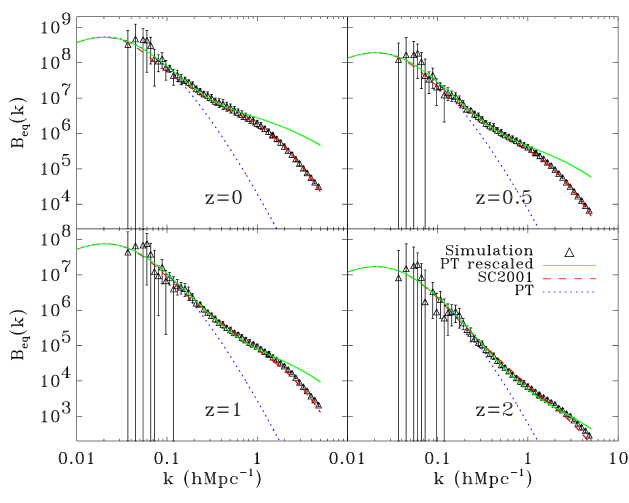
In Fig. (1) the bispectrum of equilateral triangles of simulations is plotted against tree-level perturbation theory, our model Eq. (10) and the SC2001 for reference. The rescaled tree-level perturbation theory agrees with simulations remarkably well at scales Mpc at . The range of scales in agreement also keeps increasing at higher redshift, reaching Mpc at .
In the quasi-nonlinear regime at large scales of Mpc at , Eq. (10) (our model) differs little from the tree-level perturbation theory as desired, while the suspicious lowering of SC2001 is clearly seen at low redshifts. Due to the large cosmic variance, it is not yet possible to tell which model is better.
Our model predicts too much power at scales in the strongly nonlinear regime, where the bispectrum of the simulations begins to display a power-law behaviour. The breakdown can be attributed either or both of the two principal weaknesses in our consideration: either Eq. (8) is simply too rough, or the correlation between window functions at different values of is not negligible.
3.2 Other Configurations
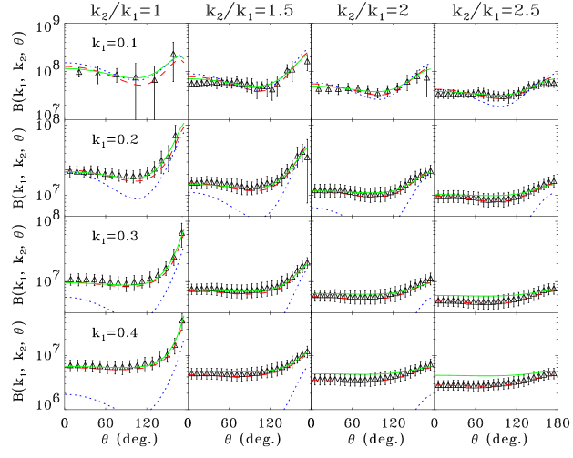
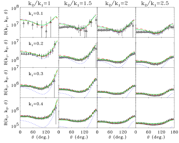
The extra complexity of bispectrum over the power spectrum is that it possesses angular dependence as well as scale dependence. Comparison of simulations with models are drawn in Fig. (2) and (3) for respectively.
It is very clear that the our model agrees much better with the simulations at higher redshift than the alternatives we considered. It is also observed that Eq. (10) is more accurate when the ratio ; within this range the variation with also matches the simulation results rather well. The major problem of our model for very tilted triangles is that if we expand with Legendre polynomials then it has a very low quadrupole moment (Szapudi 2004).
The overall performance of Eq. (10), especially at high redshift, is comparable with the perturbation theory at one-loop level although it is far simpler to implement. In fact, as a quick check we realize that the reduced bispectrum of our model is very similar to the one-loop results demonstrated in Scoccimarro et al. (1998), but emerges in a much more straightforward way using our rescaling ansatz.
4 Discussion
Following the path pioneered by Hamilton et al. (1991) and Peacock & Dodds (1996), we deploy a scale transformation argument to construct a well-behaved model of the bispectrum of dark matter fluctuations which is valid in the quasi-linear and intermediate nonlinear regimes. On the basis of the tests we have been able to perform, the resulting approximation seems to work exceptionally well, although we are somewhat hampered by numerical limitations. A full assessment of the precision and reliability of this idea will have to wait until simulations of even larger size and higher resolution than the VLS are available. Nevertheless, the important point may lie even deeper than the pragmatic usefulness of this as a simplifying ansatz. The scale transformation of Eq. (1) or (2) may contain more physical meaning than has been previously thought, and it may not after all be the case that higher-order correlation functions in the non-linear regime necessarily pose such fierce analytical and numerical challenges as has generally been asssumed.
The tree-level bispectrum is fully determined by the linear power spectrum, while the success of our model seems to tell us that the nonlinear bispectrum is governed by the nonlinear power spectrum. It therefore seems possible that having the power spectrum at hand, one can accurately derive the bispectrum of a broad range of configurations using only the knowledge that it was generated by gravitational physics.
It is well known that a Gaussian random field is fully described by its power spectrum, but does a non-Gaussian field evolved by gravity from Gaussian initial conditions also possess this feature at some level? It will be very interesting to test this idea by seeing if the trispectrum can also be obtained by rescaling tree-level perturbation theory. More fundamentally, if gravitational interactions do manage to act in such a way then why is it that the simple scale transformation, Eq. (2), manages to capture so much complicated physics?
Acknowledgment
JP acknowledges the fellowship of the One Hundred Talents program of CAS, this work is also partly support by NSFC under grant 10643002 and by PPARC through grant PPA/G/S/2000/00057. IS acknowledges support from grants NSF AST02-06423, NSF AMS04-0434413 and NASA NNG06GE71G. The simulations in this paper were carried out by the Virgo Supercomputing Consortium using computers based at Computing Centre of the Max-Planck Society in Garching and at the Edinburgh Parallel Computing Centre.
References
- [1] [] Caldwell R.R., Juszkiewicz R., Steinhardt P.J., Bouchet F.R., 2001, ApJ, 547, L93
- [2] [] Coles P., Chiang L.-Y., 2000, Nat, 406, 376
- [3] [] Colombi S., Bernardeau F., Bouchet F.R., Hernquist L, 1997, MNRAS, 287, 241
- [4] [] Cooray A., Sheth R., 2002, Phys. Rep., 371, 1
- [5] [] Fosalba P., Pan J., Szapudi I., 2005, ApJ, 632, 29
- [6] [] Goroff M.H., Grinstein B., Rey S.-J., Wise M.B., 1986, ApJ, 311, 6
- [7] [] Hamilton A.J.S., Kumar P., Lu E., Matthews A., 1991, ApJ, 374, L1
- [8] [] Hou Y.H., Jing Y.P., Zhao D.H., Börner G., 2005, ApJ, 619, 667
- [9] [] Jain B., Mo H.J., White S.D.M., 1995, MNRAS, 276, L25
- [10] [] MacFarland T., Couchman H.M.P., Pearce F.R., Pichlmeier, 1998, New Astronomy, 3, 687
- [11] [] McDonald P., 2007, Phys. Rev. D., 75, 043514
- [12] [] Nityananda R., Padmanabhan T., 1994, MNRAS, 271, 976
- [13] [] Peacock J.A., Dodds S.J., 1996, MNRAS, 280, L19
- [14] [] Peebles P.J.E., 1980, The Large Scale Structure of the Universe. Princeton University Press, Princeton, New Jersey
- [15] [] Scoccimarro R., 2000, ApJ, 544, 597
- [16] [] Scoccimarro R., Colombi S., Fry J.N., Frieman J.A., Hivon E., Melott A.L., 1998, ApJ, 496, 586
- [17] [] Scoccimarro R., Couchman H.M.P., 2001, MNRAS, 325, 1312
- [18] [] Scoccimarro R., Frieman J.A., 1999, ApJ, 520, 35
- [19] [] Scoccimarro R., Sheth R.K., Hui L., Jain B., 2001, ApJ, 546, 20
- [20] [] Smith R.E. et al., 2003, MNRAS, 341, 1311
- [21] [] Smith R.E., Watts P.I.R., Sheth R.K., 2006, MNRAS, 365, 214
- [22] [] Szapudi I., 2004, ApJ, 605, L89
- [23] [] Szapudi I., Kaiser N., 2003, ApJ, 583, L1
- [24] [] Takada M., Jain B., 2003, MNRAS, 340, 580
- [25] [] Watts P.I.R., Coles, P., 2003, MNRAS, 338, 806