Group velocity of gravitational waves
in an expanding universe

Abstract

The group velocity of gravitational waves in a flat Friedman-Robertson-Walker universe is investigated. For plane waves with wavelength well inside the horizon, and a universe filled with an ideal fluid with the pressure to density ratio less than 1/3, the group velocity is greater than the velocity of light. As a result, a planar pulse of gravitational waves propagating through the universe during the matter/dark energy dominated era arrives to the observer with the peak shifted towards the forefront. For gravitational waves emitted by inspiralling supermassive black holes at the edge of the observable universe, the typical shift that remains after the effects of nonplanarity are suppressed is of order of ten picoseconds.

1 Introduction

Recent efforts in the construction of large detectors of gravitational waves based on laser interferometry (for a review, see [1]) revived interest in investigations of emission, propagation and detection of gravitational waves. Topics that have been studied in some detail in the past include propagation of weak gravitational waves in a Friedman-Robertson-Walker (FRW) universe [2, 3, 4, 5]. The main result is that the waves do not obey Huygens’ principle unless the universe is filled with pure radiation (so that its scalar curvature is zero). Otherwise there appears a ’tail’ in the Green’s function, coming from the backscattering of waves on the spacetime curvature. This contrasts with the behavior of the electromagnetic waves, whose ’tail’, if present, consists of pure gauge.

A kinematic characteristic often used in the description of wave propagation is the group velocity. Strictly speaking, it is defined for modulated waves only, as the velocity with which ’wave groups’ travel through space. However, one commonly speaks of the group velocity of wave pulses of limited duration, too, referring to the velocity of the peak of the envelope of the pulse. (For compact pulses, this can be identified with the signal velocity, defined as the velocity with which the main part of the signal arrives to the observer [6].) Here we address the question what is the group velocity of gravitational waves in a flat FRW universe. We restrict ourselves to a flat 3-geometry because it is easier to deal with than a closed or open one, and is preferred by observations. From the results on the validity of Huygens’ principle it follows that if the universe is filled with pure radiation, plane gravitational waves advance as a whole with the velocity of light (along null geodesics with respect to the background metric). In this case the group velocity is, of course, also the velocity of light. For other kinds of cosmic environment the group velocity is presumably different; moreover, while the ’tail’ of the Green’s function lays entirely inside the light cone, there is no a priori reason for the 4-vector of the group velocity to lay inside it, too. A superluminal group velocity does not imply violation of causality since the information carried by a pulse arrives to the observer with the forefront, which travels with the velocity of light (as follows from the Hadamard discontinuity formalism, see [7]). This is similar to what happens when light passes through a medium with anomalous dispersion. As demonstrated experimentally, a pulse of light can propagate, without being significantly distorted, even with negative group velocity [8]. However, no problem with causality arises since in a dispersive medium, too, the forefront of a pulse travels with the velocity of light [6].

In section 2 we compute the group velocity of gravitational waves using a well-known formula from optics, in section 3 we make sure that the formula can be applied to the problem under study, and investigate its subtleties, within the theory of wave propagation in a time-dependent medium, and in section 4 we discuss the results. We use the signature of metric tensor $(-,+,+,+)$ and a system of units in which $c=G=1$.

2 Group velocity: calculation

Consider weak gravitational waves propagating in a flat FRW universe. The background metric is

$$ds^{2}=a^{2}\left(-dt^{2}+d{\bf x}^{2}\right),$$

where $t$ is conformal time, $x^{i}$ are comoving coordinates and $a=a(t)$ is the scale parameter. Gravitational waves are described by the perturbation to the metric of the form

$$a^{2}e_{ij}dx^{i}dx^{j}$$

where $e_{ij}$ is the traceless transversal part of the total perturbation, $e_{ii}=e_{ij,j}=0$. Denote the derivative with respect to $t$ by an overdote. The linearized Einstein equations without anisotropic stress yield (see, for example, [9])

$$\ddot{e}_{ij}+2H\dot{e}_{ij}-\triangle e_{ij}=0,$$

where $H=\dot{a}/a$ is the Hubble parameter. After passing from $e_{ij}$ to $E_{ij}=ae_{ij}$, one arrives at an equation in which the damping term is traded for a term with an external field. The equation reads

$$\ddot{E}_{ij}-\triangle E_{ij}+VE_{ij}=0,$$ (1)

where

$$V=-\dot{H}-H^{2}.$$ (2)

Suppose the universe is filled with a perfect fluid (possibly, including dark energy) and denote the density of the fluid by $\rho$ and the pressure of the fluid by $p$. Then,

$$H^{2}=\frac{8\pi}{3}\rho a^{2},\ \ \dot{H}=-\frac{4\pi}{3}(\rho+3p)a^{2},$$

so that

$$V=-\frac{4\pi}{3}(\rho-3p).$$ (3)

For a mixture of nonrelativistic matter ($p\ll\rho$), radiation ($p=\rho/3$) and dark energy ($p=-\rho$) one obtains $V\leq 0$, with the equality valid only if the universe is filled with pure radiation. For $E_{ij}$, we have a wave equation in flat spacetime, with a time-dependent dispersion relation

$$\omega=\sqrt{k^{2}+V},$$ (4)

where $\omega$ is frequency and $k$ is wave number (the magnitude of the wave vector). Suppose $\omega$ is real, that is, there holds either $V=0$ or $V<0$ and $k>|V|$ (the wavelength is less than the Jeans length). Then, the field $E_{ij}$ is in an oscillatory regime and one can ask how fast does it propagate. According to the textbook formula (see, for example, [10]), the group velocity in a medium with an isotropic dispersion relation is $v=\partial_{k}\omega$. This yields

$$v=\frac{k}{\sqrt{k^{2}+V}},$$ (5)

so that from $V\leq 0$ we have $v\geq 1$. Note that $v=1/v_{ph}$, where $v_{ph}=\omega/k$ is the phase velocity.

When computing $v$, we have ignored the fact that $\omega$ depends on $t$. However, the formula $v=\partial_{k}\omega$, supposed to be valid for $\omega=\omega(k)$, should stay valid also for $\omega=\omega(k,t)$ if the period of the oscillations of the field is much less than the time within which $\omega$ varies considerably. The period is $2\pi/\omega$ and the time scale of the variation of $\omega$ is $\omega/|\dot{\omega}|$, therefore (5) must be supplemented by the condition

$$\frac{|\dot{\omega}|}{\omega^{2}}\ll 1.$$ (6)

After inserting here from (4) we find

$$k^{2}\gg|V|+|\dot{V}|^{2/3}.$$

The universe is dominated first by radiation, then by matter, and then by dark energy, with the function $a(t)$ subsequently of the form $a\propto t$, $(t-t_{0})^{2}$ and $(t_{1}-t)^{-1}$. When using these functions to compute $V(t)$, we find that in the first era, as we already know, $V=0$, and in the next two eras $V\sim-\Delta t^{-2}$, where $\Delta t=t-t_{0}$ and $t_{1}-t$ in the second and third era respectively. The time $\Delta t$ approximately equals the horizon length, if ’horizon’ is understood as particle horizon in the matter dominated era and event horizon in the dark energy dominated era. For $V\sim-\Delta t^{-2}$ there holds $\dot{V}\sim\pm\Delta t^{-3}$, so that the two terms in the condition for $k$ are of the same order of magnitude. As a result, the condition simplifies to

$$k^{2}\gg|V|.$$ (7)

From $V\sim-\Delta t^{-2}$ we find $k\gg\Delta t^{-1}\sim$ (horizon length)^-1; thus, in order that a wave packet propagates with the group velocity (5), its mean wavelength must lay well within the horizon. For such packets, the group velocity is close to 1, with the correction of the form

$$\Delta v=-\frac{V}{2k^{2}}.$$ (8)

Light signals (particles moving along null geodesics with respect to the background metric) have coordinate velocity 1. Thus, the constraint $v\geq 1$ means that the gravitational waves either propagate with the velocity of light or are superluminal. The former case occurs in the radiation dominated era and the latter in the matter/dark energy dominated era. When combining equations (3) and (8), we find that the group velocity differs from the velocity of light by

$$\Delta v=\frac{4\pi}{3}(\rho-3p)\varkappa^{-2},$$

where $\varkappa=k/a$ is the true wave number. For an estimate, suppose the universe is filled with incoherent dust ($p=0$). Then $\rho\sim\tau^{-2}$, where $\tau$ is cosmological time, and the correction to $v$ is of order $(\varkappa\tau)^{-2}$. As a source of gravitational waves, consider a binary system consisting of two black holes with masses $M\sim 10^{6}M_{\bigodot}$, orbiting around each other with the period $T\sim 10^{4}s$. (The period drops to this value about a month before the merger.) Suppose, furthermore, that the system is at the edge of the observable universe, at the distance $l\sim 3$ Gpc from Earth. The time it takes for a packet of gravitational waves to propagate from the binary to Earth is $\tau_{prop}\sim\tau\sim 10$ Gy, and the time by which the peak of the packet arrives earlier due to the correction to $v$ is

$$\Delta\tau\sim(\varkappa\tau)^{-2}\tau_{prop}\sim\frac{T^{2}}{(2\pi)^{2}\tau}\sim 10^{-11}\mbox{s}.$$

For a universe with the actual values of cosmological parameters, $H_{0}=71$ km s^-1 Mpc^-1, $\Omega_{m}=0.26$ and $\Omega_{\Lambda}=0.74$, and a source with the period $T=1$ hour at the redshift of the most distant quasar, $z=6.4$, a detailed calculation yields $\Delta\tau=6.6\times 10^{-11}$ s.

3 Group velocity: theory

Consider a field $u$ satisfying the same equation as $E_{ij}$,

$$\ddot{u}-\triangle u+Vu=0.$$ (9)

This can describe gravitational waves in an expanding universe as well as light in a homogeneous time-dependent optical medium. Thus, the following considerations are only loosely related to general relativity; instead, one can view them as a discussion of a special problem of optics.

3.1 Waves with definite wavelength

Choose $u$ in the form of a plane wave with a definite wavelength propagating along the $x$-axis, $u=U(t)e^{ikx}$. The wave number $k$ can now assume any real value, however, for our purposes it is sufficient to suppose as before $k>0$. From (9) we obtain

$$\ddot{U}+\omega^{2}U=0,$$ (10)

with the function $\omega=\omega(k,t)$ defined in (4). If we exchange $t$ with $x$ and $\omega$ with $k$, we obtain an equation for monochromatic light in a static inhomogeneous medium; and if we replace, in addition, $\omega$ by $E$ (the energy of the particle) and $k$ by $p$ (the momentum of the particle), we obtain Schrödinger equation in one dimension with a modified relation between $p$ and $E$, $p=\sqrt{E^{2}+V}$ instead of $p=\sqrt{2(E-V)}$.

For light propagating in a medium with dispersion relation $\omega=\omega(k,t)$, the high-frequency condition (6) defines the geometrical optics approximation. An analogical condition is known to define quasiclassical, or WKB, approximation in quantum mechanics [11], and geometrical optics approximation in a static inhomogeneous medium in optics [12]. To obtain an approximate expression for $U$, write $U=e^{-i\psi}$ and expand the complex phase $\psi$ in the powers of $\omega^{-1}$. If we denote the terms of the order minus one and zero by $\psi_{0}$ and the terms of the first order by $\Delta\psi$, we have (see the corresponding formulas in [11])

$$\psi_{0}=\int\omega dt-\frac{i}{2}\log\omega,\ \ \Delta\psi=-\frac{\dot{\omega}}{4\omega^{2}}-\frac{1}{8}\int\frac{\dot{\omega}^{2}}{\omega^{3}}dt.$$ (11)

The signs in these expressions are chosen in such a way that the wave propagates in the positive $x$-direction. The first expression determines the oscillating field in the geometrical optics approximation, and the second expression can be included into the slowly varying amplitude and regarded as the post-geometrical optics correction to it.

If the dispersion relation assumes the form (4), the condition (6) for $\omega$ implies the condition (7) for $k$. (This holds irrespective of the form of $V(t)$. In general, we have also condition $k^{2}\gg|\dot{V}|^{2/3}$, however, it can be skipped if we choose $V\sim-\Delta t^{-2}$.) With $k$’s satisfying the condition (7), the dispersion relation can be written approximately as

$$\omega=k+\frac{V}{2k}.$$ (12)

The fact that we have replaced the condition for $\omega$ by the condition for $k$ suggests that the concept of geometrical optics approximation must be reconsidered. The small parameter of the theory is $(k\Delta t)^{-1}$, where $\Delta t$ is the time scale of the variation of $V$, rather than $(\omega\delta t)^{-1}$, where $\delta t$ is the time scale of the variation of $\omega$, therefore it is advisable to expand all quantities in the powers of $k^{-1}$ rather than $\omega^{-1}$. In particular, the approximate expression for $\omega$ should be written $\omega=\omega_{0}+\Delta\omega$, with the frequency in the geometrical optics approximation $\omega_{0}=k$ and the post-geometrical optics correction to it $\Delta\omega=V/(2k)$. This yields

$$\psi_{0}=kt-\frac{i}{2}\log k,\ \ \Delta\psi=\frac{1}{2k}\int Vdt.$$ (13)

The previously obtained expression for $\Delta\psi$ does not contribute here since it is of order $k^{-3}$. Note, however, that it would contribute if we used cosmological time instead of conformal, since then it would be of order $k^{-1}$.

3.2 Group velocity of a Gaussian packet with infinitesimal dispersion

From plane waves with a definite wavelength one can form a planar wave packet

$$u(x,t)=\int\limits_{-\infty}^{\infty}a(K)e^{-i\psi(K,t)+iKx}dK,$$ (14)

where $a$ is an overall amplitude peaked at the given wave number $k$ and differing significantly from zero only in an interval of a size $\sigma\ll k$. Note that the integral contains modes with all $k$’s, and we have derived formulas for $\psi(k,t)$ only for $k$ positive and large enough to satisfy the high-frequency condition. However, the modes with $k$ either positive and small or negative do not have significant effect on the results in the limit we are interested in, therefore we can describe them by an extrapolated formula for large positive $k$.

Define the envelope of the wave packet as the curve $|u(x,t)|$ at fixed $t$, and the group velocity $v$ as the velocity with which the peak of the envelope moves along the $x$-axis. That is,

$$v=\dot{x}_{M},$$ (15)

where $x_{M}$ is the value of $x$ at which the function $|u(x,t)|$ has maximum at fixed $t$. To obtain an approximate expression for $v$, let us adopt two simplifications. First, consider a Gaussian packet,

$$a_{G}=\frac{1}{\sqrt{2\pi}\sigma}\exp\left(-\frac{\Delta K^{2}}{2\sigma^{2}}\right),$$ (16)

and second, expand the phase in the powers of $\Delta K=K-k$,

$$\psi(K,t)=\psi+\xi\Delta K+\frac{1}{2}\eta\Delta K^{2}+\frac{1}{6}\zeta\Delta K^{3}+\ldots,$$ (17)

where $\psi=\psi(k,t)$, $\xi=\partial_{k}\psi$, $\eta=\partial^{2}_{k}\psi$, $\zeta=\partial^{3}_{k}\psi$, $\ldots$, and compute $v$ in the linear approximation in which the expansion is truncated after the $\xi$-term.

Let $\cal U$ be the function obtained by factorizing out the quickly oscillating phase factor from $u$, $u=e^{-i\psi+ikx}\cal U$. For a Gaussian packet, $\cal U$ in the linear approximation is

$${\cal U}_{lin}=e^{-\frac{1}{2}\sigma^{2}(x-\xi)^{2}},$$

and its magnitude is

$$|{\cal U}_{lin}|=e^{-\frac{1}{2}\sigma^{2}[(x-\xi_{R})^{2}-\xi_{I}^{2}]},$$

where the indices $R$ and $I$ denote the real and imaginary part of the quantity in question. We can see that the wave packet in $x$-space is Gaussian, like in $k$-space, with the width $\sigma_{x}=1/\sigma$ and the peak located at

$$x_{M}=\xi_{R}.$$ (18)

For a general time-dependent medium we have

$$\xi_{0R}=\int\partial_{k}\omega dt,\ \ \Delta\xi_{R}=-\frac{1}{4}\partial_{k}\left(\frac{\dot{\omega}}{\omega^{2}}+\frac{1}{2}\int\frac{\dot{\omega}^{2}}{\omega^{3}}dt\right).$$

From the first expression we obtain the leading term in $v$, which is just the standard group velocity cited in the previous section,

$$v_{0}=\partial_{k}\omega.$$ (19)

The second expression yields the correction

$$\Delta v=-\frac{1}{4}\partial_{k}\left(\frac{\ddot{\omega}}{\omega^{2}}-\frac{3\dot{\omega}^{2}}{2\omega^{3}}\right).$$ (20)

For a medium with the dispersion relation (4) we have

$$\xi_{0R}=t,\ \ \Delta\xi_{R}=-\frac{1}{2k^{2}}\int Vdt,$$

which yields $v=1+\Delta v$ with $\Delta v$ given by equation (8). In this case the group velocity is given, within the current accuracy, entirely by the formula $v=\partial_{k}\omega$.

If we include higher order terms into the $\Delta K$-expansion of $\psi$ into the calculation, we obtain corrections of order $\sigma^{2}$, $\sigma^{4}$, $\ldots$ to $\cal U$ near $x=x_{M}$, producing corrections of order $\sigma^{2}$, $\sigma^{4}$, $\ldots$ to $x_{M}$. Thus, the values of $x_{M}$ and $v$ obtained for a Gaussian packet in the linear approximation can be viewed as exact values in the limit $\sigma=0$ (vanishing width of the packet in $k$-space). Equivalently, one can speak of the limit $\sigma_{x}=\infty$ (infinite width of the packet in $x$-space).

3.3 Effects of finite dispersion and nongaussianity

Consider first a Gaussian packet beyond the linear approximation. To find the first correction to the expression for $x_{M}$ obtained before may seem trivial, because if we include the $\eta$-term into $\psi(K,t)$, we arrive at an integral that can still be calculated explicitly. However, as shown in the appendix, the correction contains also a contribution of the $\zeta$-term which is comparable with the contribution of the $\eta$-term or greater. After taking into account this contribution we find that (see equation (A-13) and the comment preceding equation (A-14))

$$\mbox{the first correction to}\ x_{M}\sim\frac{1}{\kappa}\eta_{R}\sigma^{2},$$

where $\kappa$ is a typical interval of $k$ within which $\omega$ varies, $\kappa=\omega/|\partial_{k}\omega|$. If $\Delta v$ is to stay the leading correction to $v_{0}$, the expression on the r.h.s. must be much smaller in the absolute value than the correction to $x_{M}$ from which $\Delta v$ has been computed,

$$\frac{1}{\kappa}|\eta_{R}|\sigma^{2}\ll|\Delta\xi_{R}|.$$ (21)

Of course, the condition is relevant only if the effect of higher corrections to $x_{M}$ coming from finite $\sigma$ is negligible; that is to say, if the perturbation theory with small parameter $\sigma$ can be employed. The corresponding conditions are summarized in equation (A-11). It turns out that $\sigma$ is small enough if it is much less, at the same time, than $1/|\xi_{I}|$, $1/\sqrt{|\eta_{R}|}$ and $\kappa$.

For nongaussian packets, write the linear part of $\cal U$ as

$${\cal U}_{lin}=\int\limits_{-\infty}^{\infty}b(K,t)e^{i\Delta KX}dK,$$

where $b(K,t)=ae^{\xi_{I}\Delta K}$ and $X=x-\xi_{R}$. The additional correction to $x_{M}$, supplementing that from which $\Delta v$ has been computed, equals the value of $X$ at which the function $|{\cal U}(X,t)|$ has maximum. Denote this value by $X_{M}$. Since $b$ depends on $t$, $X_{M}$ is expected to depend on $t$, too; and since $t$ appears in $b$ through $\xi_{I}$, which has the same physical dimension as $X_{M}$, the leading time-dependent term in $X_{M}$ is expected to be proportional to $\xi_{I}$ with a coefficient of order 1. Thus, if one considers a generic nongaussian packet and wants $\Delta v$ to be the dominant correction to $v$, one must have, in addition to small $\sigma$, also small $|\xi_{I}|$. A term proportional to $\xi_{I}$ is present in $X_{M}$, for example, if the packet has amplitude $(1+\alpha\Delta K/\sigma)a_{G}$ with $\alpha=const$. Such packet has two maxima placed symmetrically with respect to the center, located at the points

$$X_{M}=\pm\left[const+\frac{1}{\alpha}\xi_{I}+O(\sigma)\right].$$ (22)

On the other hand, it is easy to construct a wide class of packets for which the time-dependent part of $X_{M}$ is exactly zero in the linear approximation. For that purpose, we can use the argument of [10] with exchanged space and time dimensions. Suppose $a$ equals a real nonnegative function modulo a phase factor with the phase proportional to $\Delta K$, $a=Ae^{iq\Delta K}$ with $A\geq 0$ and $q=const$. Then

$$|{\cal U}_{lin}|^{2}=\int dKdK^{\prime}B(K,t)B(K^{\prime},t)\cos[(K-K^{\prime})(X+q)],$$

where $B(K,t)=Ae^{\xi_{I}\Delta K}$, and this has obviously maximum at $X_{M}=-q$.

A general analysis of nongaussian packets can be found in the appendix. The estimate of the time-dependent part of $X_{M}$ in equation (A-12) implies that the conditions under which $\Delta v$ dominates other corrections to $v$ are

$$|\xi_{I}|\ \mbox{and}\ |\eta_{R}|\sigma\ll|\Delta\xi_{R}|.$$ (23)

In addition to that, one must again satisfy conditions (A-11) in order that the perturbation theory with small parameter $\sigma$ is applicable.

In a general time-dependent medium, the quantities entering the constraints (A-11), (21) and (23) are of order

$$\Delta\xi_{R}\sim\frac{1}{\kappa\omega\delta t},\ \ \xi_{I}\sim\frac{1}{\kappa},\ \ \eta_{R}\sim\frac{\omega\delta t}{\kappa^{2}}.$$ (24)

From these estimates we find that the perturbation theory is justified only if $\sigma\ll(\omega\delta t)^{-1/2}\kappa$, and $\Delta v$ cannot be the leading correction to $v_{0}$ for a general packet. However, it becomes the leading correction if the packet is Gaussian and has $\sigma\ll(\omega\delta t)^{-2}\kappa$. Note that an analogical condition for a quantum mechanical particle in an external potential, obtained by flipping over space and time directions and identifying wave characteristics with mechanical ones, yields a packet that is much larger than the typical distance on which the potential varies. Thus, the post-WKB correction to $v$ has no relevance for the description of the motion of a quantum mechanical particle in an external potential.

For a medium with dispersion relation (4), we must modify the theory slightly in order that the results of the appendix remain valid. Namely, we must define the phase $\psi$ in the geometrical optics approximation in a different, and perhaps more natural, way, with omitted $\log k$. This yields an expression for $U$ stripped of the overall factor $1/\sqrt{k}$, which can be regarded as absorbed into $a$. Using this ’reduced’ definition of $\psi$, and assuming $V\sim-\Delta t^{-2}$, we find that the relevant quantities are of order

$$\Delta\xi_{R}\sim k^{-2}\Delta t^{-1},\ \ \xi_{I}\sim k^{-3}\Delta t^{-2},\ \ \eta_{R}\sim k^{-3}\Delta t^{-1},$$ (25)

(The second estimate comes from $\psi_{I}=-V/(4k^{2})$.) If we also take into account that $\kappa=k$, we conclude that both sets of constraints (A-11) and (23) are satisfied provided $\sigma\ll k$, which we have assumed from the very start. Thus, for the ’cosmological’ dispersion relation, the quantity $\Delta v$ coming from the post-geometrical optics contribution to $\psi$ is the dominant correction to $v$ for all wave packets whose width in $k$-space is small in comparison with the typical value of $k$.

3.4 Exact solution

To support our conclusions, let us construct an exact solution to equation (9). Suppose

$$V=-\frac{2}{t^{2}}.$$ (26)

As seen from (2), $V$ assumes this form for gravitational waves in a dust universe (which expands after the law $a\propto t^{2}$). First we find solutions with definite wavelength. If we pass from $U$ to $U/t$ and from $t$ to $kt$, (10) transforms into the equation for spherical Bessel function with $l=1$. Moreover, we can see from (13) with omitted logarithm that the asymptotics of $U$ for $kt\gg 1$ is $U=e^{-i[kt+1/(kt)]}$. This yields

$$U=-kth_{1}^{(2)}(kt)=\left(1-\frac{i}{kt}\right)e^{-ikt}.$$

Next we form a wave packet with the amplitude $Ka_{G}/k$. The function $\cal U$ is

$${\cal U}=[1+i(p-qs)]e^{-\frac{1}{2}s^{2}},$$

where $s=\sigma(x-t)$, $p=1/(kt)$ and $q=\sigma/k$. After inserting this into the condition $\partial_{s}|{\cal U}|^{2}(s_{M})=0$ we find

$$\left[1-q^{2}+(p-qs_{M})^{2}\right]s_{M}+pq=0.$$ (27)

By definition $s_{M}=\sigma(x_{M}-t)$, therefore the equation for $s_{M}$ determines the worldline of the peak of the packet $x=x_{M}(t)$. In fig. 1 this worldline is depicted for $k=1$ and $\sigma=1/3$.

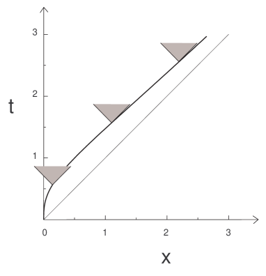
Figure 1: Gravitational wave packet in a dust universe

At the beginning, the peak of the packet stays within the light cone, but then it moves out. This is consistent with the sign $\Delta v$ assumes at late times according to (8).

3.5 Spherical packet

Consider equation (9) with the source $4\pi j$. If we ignore the field $V$, the solution is

$$u^{(0)}({\bf r},t)=\int\frac{1}{R}j({\bf r}^{\prime},t-R)d^{3}x^{\prime},$$ (28)

where $R=|{\bf r}-{\bf r}^{\prime}|$. Suppose the source is nonrelativistic. In the wave zone, $u^{(0)}$ can be written as

$$u^{(0)}\doteq\frac{1}{r}(f+{\bf n}\ .\ \dot{\bf g})+\frac{1}{r^{2}}{\bf n}\ .\ {\bf g},\ \ f=\int j({\bf r}^{\prime},\tau)d^{3}x^{\prime},\ \ {\bf g}=\int j({\bf r}^{\prime},\tau){\bf r}^{\prime}d^{3}x^{\prime},$$

where $\tau=t-r$ and ${\bf n}={\bf r}/r$. The magnitude of $u^{(0)}$ is

$$|u^{(0)}|\doteq\frac{1}{r}(|f|+{\bf n}\ .\ {\bf G}_{1})+\frac{1}{r^{2}}{\bf n}\ .\ {\bf G},\ \ {\bf G}=\frac{1}{|f|}\mbox{Re}(f{\bf g}^{*}),\ \ {\bf G}_{1}=\frac{1}{|f|}\mbox{Re}(f\dot{\bf g}^{*}).$$

We are interested in the radial coordinate $r_{M}^{(0)}$ at which $|u^{(0)}|$ has maximum for the given direction of the propagation of the packet $\bf n$. To compute this quantity, we expand the derivative

$$\partial_{r}|u^{(0)}|\doteq-\frac{1}{r}\left(|f|\dot{\ }+{\bf n}\ .\ \dot{\bf G}_{1}\right)-\frac{1}{r^{2}}\left(|f|+{\bf n}\ .\ {\bf G}_{1}+{\bf n}\ .\ \dot{\bf G}\right)$$

around $r_{\cal M}=t-\tau_{\cal M}$, where $\tau_{\cal M}$ is the value of $\tau$ at which the function $|f|$ has maximum. In fact, we can put $r=r_{\cal M}$ in the argument of all functions except for $|f|\dot{\ }$, which we must expand up to the first order in $\Delta r=r-r_{\cal M}$. After replacing $r_{\cal M}$ by $t$ we obtain

$$\Delta r_{M}^{(0)}=\frac{1}{|f|_{\cal M}\mbox{\hskip-7.11317pt\large$\ddot{}$}\hskip 7.11317pt}\left[{\bf n}\ .\ {\dot{\bf G}}_{1{\cal M}}+\frac{1}{t}\left(|f|_{\cal M}+{\bf n}\ .\ {\bf G}_{1{\cal M}}+{\bf n}\ .\ \dot{\bf G}_{\cal M}\right)\right],$$ (29)

where the index ${\cal M}$ indicates that the quantity in question is to be taken at $r=r_{\cal M}$ (or, equivalently, at $\tau=\tau_{\cal M}$). By differentiating this with respect to $t$ we finally find that the correction to the group velocity coming from the nonplanarity of the wave packet is

$$\Delta v^{(0)}=-\frac{1}{|f|_{\cal M}\mbox{\hskip-7.11317pt\large$\ddot{}$}\hskip 7.11317ptt^{2}}\left(|f|_{\cal M}+{\bf n}\ .\ {\bf G}_{1{\cal M}}+{\bf n}\ .\ \dot{\bf G}_{\cal M}\right).$$ (30)

To estimate the dominant term, note that $|f|_{\cal M}\mbox{\hskip-7.11317pt\large$\ddot{}$}\hskip 7.11317pt\sim-|f|_{\cal M}/\sigma_{r}^{2}$, where $\sigma_{r}$ is the dispersion of the packet in the radial coordinate. This yields

$$\Delta v^{(0)}\sim\frac{\sigma_{r}^{2}}{t^{2}}.$$

We can see that the group velocity of the radiation emitted by a compact source is superluminal even without a time-dependent medium, merely due to the fact that the factor $1/r$ shifts the maximum of the envelope of the packet the more backwards the closer the packet to the source. This is demonstrated in Fig. 2.

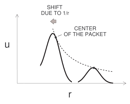
Figure 2: Superluminal velocity of a spherical wave packet

If we put the field $V$ back into the wave equation, we obtain, in addition to $\Delta v^{(0)}$, another contribution to the group velocity $\Delta v_{V}$. As we shall see, nonplanarity has significant effect on the propagation of the packet, but in relation to $\Delta v_{V}$ we can make use of the fact that in a sufficiently small domain any spherical wave can be replaced by planar, and identify $\Delta v_{V}$ with the contribution to the group velocity $\Delta v$ computed before. To estimate the relative size of the corrections $\Delta v_{V}$ and $\Delta v^{(0)}$, consider again, as in section 2, a dust universe. Then $\Delta v_{V}\sim(kt)^{-2}$, and since the dispersion in $x$-space $\sigma_{r}$ equals approximately the inverse of the dispersion in $k$-space $\sigma$, we have

$$\frac{\Delta v_{V}}{\Delta v^{(0)}}\sim\frac{\sigma^{2}}{k^{2}}\ll 1.$$ (31)

From (30) we can estimate the next-to-leading term in $\Delta v^{(0)}$ as $\Delta v^{(0)}_{next}\sim v_{s}\Delta v^{(0)}$, where $v_{s}$ is the typical velocity with which the parts of the source move with respect to each other. This yields

$$\frac{\Delta v_{V}}{\Delta v^{(0)}_{next}}\sim\frac{\sigma^{2}}{v_{s}k^{2}}.$$ (32)

The leading term in $\Delta v^{(0)}$ is determined by the form of the packet in the vicinity of the peak of the envelope, and can in principle be established by the local measurement of the oscillating field. Thus, $\Delta v_{V}$ can be found from local data if it dominates $\Delta v^{(0)}_{next}$, which is the case if the velocity of the internal motion of the source is small enough, $v_{s}\ll\sigma^{2}/k^{2}$.

4 Conclusion

When inspecting the equation for gravitational waves in an expanding universe, one immediately observes that the group velocity predicted by it is superluminal provided the pressure to density ratio is less than 1/3 (which is surely the case in our universe) and the typical wavelength of the waves lays well within the horizon. The positive sign of the additional velocity $\Delta v$ is entirely the consequence of the negative sign of the ’external field’ $V$, which in turn reflects the fact that for gravitational waves there exists a finite Jeans length of order of horizon length. Note that for electromagnetic waves, $\Delta v$ is exactly zero. The reason is the conformal invariance of Maxwell action in four dimensions, which prevents the intensity of the field from having ’tails’ inside the light cone; for details, see [3]. To support our calculation of $\Delta v$, we have performed a detailed analysis of wave propagation in a time-dependent medium. The value of $\Delta v$ proved correct for plane waves, and one would expect that it will be automatically correct for spherical waves, too, since group velocity is a local characteristic and spherical waves are locally equivalent to plane ones. However, the effect is so small that the effects of nonplanarity turn out to be substantially superior to it. For gravitational waves coming from astrophysical sources, the net time shift $\Delta\tau$ caused by $\Delta v$ is at best of order of 10 ps. Such a short time would be surely hard to measure even if its beginning and end were defined by single events, which they are not. To determine $\Delta\tau$, one should reconstruct the envelope of the pulse in the vicinity of the peak with an error less by many orders of magnitude than the period of the pulse; calculate the position of the peak relative to the forefront at the moment of the formation of the pulse with the same accuracy; and separate out the effects of nonplanarity. A principal obstacle to the first step seems to be that in order to carry it out, one needs to know the imaginary part of the oscillating field, which is an auxiliary object inaccessible to the measurements. However, the analysis in the appendix suggests that the complex field can be reconstructed from the data by a suitable approximate procedure, most simply, by determining the Fourier coefficients of the real field seen in the experiment and making use of the coefficients with positive $k$’s only. While this would typically produce a much greater error than the measured effect, only the time-independent part of the position of the peak of the envelope (the quantity $s_{0}$ in the notations of the appendix) would be affected. Obviously, there is no hope that the outlined procedure to measure $\Delta\tau$ could sometimes be carried out in practice. Nevertheless, we believe that the effect is still of some interest since it contributes to our understanding of how the propagation of gravitational waves is affected by the expansion of the universe.

Acknowledgement. This work was supported by the grant VEGA 1/3042/06.

Appendix A Propagation of planar wave packets

A general planar wave packet in a time-dependent medium is described by the integral

$${\cal U}=\int\limits_{-\infty}^{\infty}a(K)e^{-i\Delta\psi+i\Delta Kx}dK,$$ (A-1)

where

$$\Delta\psi=\psi(K,t)-\psi=\xi\Delta K+\frac{1}{2}\eta\Delta K^{2}+\frac{1}{6}\zeta\Delta K^{3}+\ldots,\ \ \Delta K=K-k.$$ (A-2)

Introduce the Fourier transform of $a$,

$$\alpha(s)=\int\limits_{-\infty}^{\infty}a(K)e^{i\Delta Ks}dK.$$

If we write the exponential function in the expression for $\cal U$ as

$$e^{-i\Delta\psi+i\Delta Kx}=e^{i\Delta K{\cal X}}\left(1-\frac{i}{2}\eta\Delta K^{2}-\frac{i}{6}\zeta\Delta K^{3}+\ldots\right),$$

where ${\cal X}=x-\xi$, we find

$${\cal U}=\alpha+\frac{i}{2}\eta\alpha^{\prime\prime}+\frac{1}{6}\zeta\alpha^{\prime\prime\prime}+\ldots,$$

where the functions $\alpha$, $\alpha^{\prime\prime}$, $\ldots$ are taken at the (complex) value of the argument $s=\cal X$. Next, we expand the functions $\alpha$, $\alpha^{\prime\prime}$, $\ldots$ around the point $s_{0}$ at which $|\alpha|$ has maximum. This yields

$${\cal U}=A_{0}+A_{1}\Delta{\cal X}+\frac{1}{2}A_{2}(i\eta+\Delta{\cal X}^{2})+\frac{1}{6}A_{3}(\zeta+3i\eta\Delta{\cal X}+\Delta{\cal X}^{3})+\ldots,$$ (A-3)

where $A_{n}$ is the $n$th derivative of $\alpha$ at $s=s_{0}$ and $\Delta{\cal X}={\cal X}-s_{0}$. Suppose $a(K)$ is of the form $f(\Delta K/\sigma)/\sigma$, where $|f|$ has maximum of order 1, $f(u)$ is significantly different from zero only in the interval $|u|\lesssim 1$, and the derivatives of $f$ obey $|f^{(n)}(u)|\lesssim 1$ everywhere in the interval $|u|\lesssim 1$. For a large class of such functions (for example, for Gaussian functions with the dispersion of order $\sigma$ multiplied by appropriately normalized, but otherwise arbitrary polynomials), $\alpha(s)$ is of the form $\tilde{f}(\sigma s)$, where $\tilde{f}(u)$ has the same properties as $f(u)$. Then, the coefficients in the sum (A-3) can be estimated as

$$A_{n}=\tilde{f}^{(n)}(\sigma s_{0})\sigma^{n}\sim\sigma^{n},$$

and the sum is in fact a power series in $\sigma$. The real part of the shift $\Delta{\cal X}$ is $\Delta X=X-s_{0}$, where $X={\cal X}_{R}=x-\xi_{R}$. Here, as in section 3, we denote by $R$ and $I$ the real and imaginary part of the quantity in question. If we pass from $\Delta{\cal X}$ to $\Delta X$ in the expression for $\cal U$, we obtain a series

$${\cal U}=u_{0}+u_{1}\Delta X+u_{2}\Delta X^{2}+\ldots,$$ (A-4)

with each coefficient itself a series,

$$u_{n}=\frac{1}{n!}\sum\limits_{m=0}^{\infty}A_{n+m}\psi_{m},\ \ \psi_{0}=1,\ \ \psi_{1}=-i\xi_{I},\ \ \psi_{2}=\frac{1}{2}(i\eta-\xi_{I}^{2}),\ \ \psi_{3}=\frac{1}{6}(\zeta+3\xi_{I}\eta+i\xi_{I}^{3}),\ \ \ldots$$ (A-5)

We are interested in the shift of the peak of the wave packet $X_{M}=x_{M}-\xi_{R}$. This can be written as $X_{M}=s_{0}+\Delta X_{M}$, where $\Delta X_{M}$ is the value of $\Delta X$ at which the function $|{\cal U}|^{2}$ has maximum at fixed $t$. Extrema of $|{\cal U}|^{2}$ are zeros of the function

$$\partial_{x}|{\cal U}|^{2}\propto U_{0}+U_{1}\Delta X+U_{2}\Delta X^{2}+\ldots,\ \ U_{n}=\sum\limits_{m=0}^{n}(n+1-m)(u_{m}u_{n+1-m}^{*})_{R}.$$

For small enough $\sigma$ we expect $|{\cal U}|$ to be close to $|\alpha|$ at $X\sim s_{0}$. Then, the value of $\Delta X_{M}$ can be found by solving the equation $U_{0}+U_{1}\Delta X+U_{2}\Delta X^{2}+\ldots=0$ iteratively,

$$\Delta X_{M}^{(1)}=-\frac{U_{0}}{U_{1}}\equiv\Delta,\ \ \Delta X_{M}^{(2)}=\Delta-\frac{U_{2}}{U_{1}}\Delta^{2},\ \ \Delta X_{M}^{(3)}=\Delta-\frac{U_{2}}{U_{1}}\Delta^{2}-\left[\frac{U_{3}}{U_{1}}-2\left(\frac{U_{2}}{U_{1}}\right)^{2}\right]\Delta^{3},\ \ \ldots$$

The quantities $U_{k}$ are generically of order $\sigma^{k+1}$, except for $U_{0}$ which is of order $\sigma^{2}$. Indeed,

$$U_{0}=(u_{0}u_{1}^{*})_{R}=(A_{0}A_{1}^{*})_{R}+O(\sigma^{2}),$$

and if we fix, for the sake of simplicity, the overall phase of $\alpha$ so that $\alpha(s_{0})$ is real, we find that $A_{0}$ is real and $A_{1}$ purely imaginary. From the estimate of $U_{k}$ it follows that the term proportional to $\Delta^{n}$ in the iterative expression for $\Delta X_{M}$ is generically of order $\sigma^{n-1}$, so that the procedure is meaningful for small enough $\sigma$. Finally, we expand all terms entering $\Delta X_{M}$ in the powers of $\sigma$ to obtain

$$\Delta X_{M}=X_{M0}+X_{M1}+X_{M2}+\ldots,\ \ X_{Mn}\sim\sigma^{n}.$$ (A-6)

Note that $s_{0}$ is generically of order $1/\sigma$ (the width of the wave packet in $x$-space), therefore a power series for $\Delta X_{M}$ defines a power series for $X_{M}$, too, but starting with a term of order minus one rather than zero. If we write

$$U_{0}={\cal A}+\Delta{\cal A}+\ldots,\ \ U_{1}={\cal B}+\Delta{\cal B}+\ldots,\ \ U_{3}={\cal C}+\ldots,$$

where $\cal A$, $\cal B$ are of order $\sigma^{2}$ and $\Delta\cal A$, $\Delta\cal B$, $\cal C$ are of order $\sigma^{3}$, we find that the first two terms in the expansion of $\Delta X_{M}$ are

$$X_{M0}=-\frac{\cal A}{\cal B}\equiv\delta,\ \ X_{M1}=-\frac{1}{\cal B}(\Delta{\cal A}+\Delta{\cal B}\delta+{\cal C}\delta^{2}).$$ (A-7)

(We do not consider the case ${\cal B}=0$ which requires a separate discussion.) The expressions for $\Delta\cal A$, $\Delta\cal B$ and $\cal C$ are obtained from the expansions of first few $u$’s in the powers of $\sigma$. A straightforward computation yields

$${\cal A}=A_{0}A_{2I}\xi_{I},\ \ {\cal B}=A_{0}A_{2R}+A_{1I}^{2},\ \ \Delta{\cal A}=-\frac{1}{2}A_{0}[A_{3R}(\eta_{I}+\xi_{I}^{2})+A_{3I}\eta_{R}]+\frac{1}{2}A_{1I}\mbox{\tiny$\times$}$$ (A-8)

$$\mbox{\tiny$\times$}[A_{2R}\eta_{R}-A_{2I}(\eta_{I}-\xi_{I}^{2})],\ \ \Delta{\cal B}=(A_{0}A_{3I}-A_{1I}A_{2R})\xi_{I},\ \ {\cal C}=\frac{1}{2}(A_{0}A_{3R}+3A_{1I}A_{2I}).$$

Note that only $\xi$ and $\eta$ (the first and second derivative of $\psi$) appear here, although $\zeta$ (the third derivative) is to be included, too, into the formulas for $\cal U$ and $|{\cal U}|^{2}$, if one writes them with the accuracy needed for the calculation of $\Delta X_{M}$ up to the term $X_{M1}$. The point is that $\zeta$ enters only the term independent on $\Delta X$ in $|{\cal U}|^{2}$ and therefore plays no role in the extremization. Note, furthermore, that if $A_{2I}$ is zero (the phase of the function $\alpha$ has zero second derivative at the maximum of $|\alpha|$), $X_{M0}$ is zero and $\Delta X_{M}$ is at least of order $\sigma$. For this class of packets, $\Delta X_{M}$ can be made arbitrarily small by shrinking the packet in $k$-space. To understand why $A_{2I}$ rather than $A_{1I}$ determines $X_{M0}$, note that $A_{1I}$ can be adjusted arbitrarily by shifting the packet in $k$-space. But the shift of the packet by the distance $q$ results only in multiplication of ${\cal U}_{lin}=\alpha({\cal X})$ (the function ${\cal U}$ in the linear approximation) by the factor $e^{iq\cal X}$, which has no effect on the position of the peak of $|{\cal U}_{lin}|$ at fixed $t$. Thus, we can change $A_{1I}$ without changing $X_{M}$ in the linear approximation; and since the linear approximation is all what is needed to determine $X_{M0}$, the value of $X_{M0}$ cannot depend on $A_{1I}$.

An important special case is the Gaussian wave packet (16). The Fourier transform of a Gaussian amplitude is again Gaussian,

$$\alpha_{G}=\sqrt{2\pi}\sigma\exp\left(-\frac{1}{2}\sigma^{2}s^{2}\right).$$

Since this is real, all imaginary $A$’s vanish; and since this is an even function of $s$, with the maximum at the origin, $s_{0}=0$ and all odd $A$’s vanish, too. This implies that $X_{M0}=X_{M1}=0$ and the leading term in $\Delta X_{M}$ as well as in $X_{M}$ is $X_{M2}$. For an arbitrary packet with real nonzero $A_{0},A_{2},A_{4},\ldots$ and zero $A_{1},A_{3},\ldots$ we have

$$U_{0}=(u_{0}u_{1}^{*})_{R}=\frac{1}{6}A_{0}A_{4}(\zeta_{R}+3\xi_{I}\eta_{R})+\frac{1}{2}A_{2}^{2}\xi_{I}\eta_{R}+\ldots,\ \ U_{1}=2(u_{0}u_{2}^{*})_{R}+|u_{1}|^{2}=A_{0}A_{2}+\ldots$$

If we insert here the $A$’s for a Gaussian packet, $A_{2\nu}=(-1)^{\nu}(2\nu-1)!!\sigma^{2\nu}$, and use the resulting $U_{0}$ and $U_{1}$ in the formula $X_{M}=-U_{0}/U_{1}+\ldots$, we find

$$X_{M2}=\left(\xi_{I}\eta_{R}+\frac{1}{2}\zeta_{R}\right)\sigma^{2}.$$ (A-9)

Note that the first term can be obtained also from the analytical expression for $\cal U$ in the quadratic approximation, with the $\Delta K$-expansion of $\psi$ truncated after the $\eta$-term. In this approximation, $\cal U$ can be found from the formula for ${\cal U}_{lin}$ written down in section 3, by replacing

$$\frac{1}{\sigma^{2}}\to\frac{1}{\sigma^{2}}+i\eta.$$

This yields

$$|{\cal U}|=\frac{1}{\sqrt{A}}e^{-\frac{1}{2A^{2}}\sigma^{2}[a(X^{2}-\xi_{I}^{2})-2\xi_{I}\eta_{R}\sigma^{2}X]},$$

where $a=1-\eta_{I}\sigma^{2}$ and $A=\sqrt{a^{2}+\eta_{R}^{2}\sigma^{4}}$. The wave packet is Gaussian as in the linear approximation, but with a time-dependent width $\sigma_{x}=A/(\sqrt{a}\sigma)$ and the peak shifted by $X_{M}=\xi_{I}\eta_{R}\sigma^{2}/a$. Within the current accuracy, the factor $1/a$ in the expression for $X_{M}$ plays no role. Thus, $X_{M}$ effectively equals the first term on the right hand side of (A-9) as mentioned above.

Let us find conditions under which our perturbative approach is applicable, and estimate the time-dependent part of $X_{M}$. We are interested in this part only, because we wish to compare different contributions to $v=\dot{x}_{M}$ rather than to $x_{M}$. If we use the “reduced” definition of $\psi$, with whatever factor in $\omega$ depending only on $k$ removed from the term proportional to $\log\omega$, the time-dependent part of $X_{M}$ is just $\Delta X_{M}$. (If we left such factor in $\omega$, we would have to skip from $X_{M}$, in addition to $s_{0}$, also a part of $X_{M0}$.) As demonstrated in previous calculations, the term $X_{Mn}$ in the expansion of $\Delta X_{M}$ is a sum of products

$$\xi_{I}^{\nu_{1I}}\eta_{R}^{\nu_{2R}}\eta_{I}^{\nu_{2I}}\zeta_{R}^{\nu_{3R}}\zeta_{I}^{\nu_{3I}}\ldots\psi_{R}^{(n+1)\nu_{n+1,R}}\psi_{I}^{(n+1)\nu_{n+1,I}}\sigma^{n},\ \ \sum\limits_{mA}m\nu_{mA}=n+1,$$

multiplied by coefficients of order 1. For the real and imaginary part of the $n$th derivative of $\psi$ we have $\psi_{R}^{(n)}\sim\hat{\eta}_{R}/\kappa^{n}$ and $\psi_{I}^{(n)}\sim\hat{\xi}_{I}/\kappa^{n}$, where $\hat{\xi}=\xi\kappa$, $\hat{\eta}=\eta\kappa^{2}$ and $\kappa$ is the scale of $k$ on which $\omega$ varies. Thus, if $p_{(\nu_{R},\nu_{I})}$ is the sum of terms in $X_{Mn}$ with given $\nu_{R}=\sum\nu_{mR}$ and $\nu_{I}=\sum\nu_{mI}$ such that $n^{\prime}=2\nu_{R}+\nu_{I}\leq n+1$, we have

$$p_{(\nu_{R},\nu_{I})}\sim\hat{\xi}_{I}^{\nu_{I}}\hat{\eta}_{R}^{\nu_{R}}\frac{\sigma^{n}}{\kappa^{n+1}}.$$ (A-10)

Rewrite this as

$$p_{(\nu_{R},\nu_{I})}\sim\bigg{[}\xi_{I}(\xi_{I}\sigma)^{\nu_{I}-1}(\eta_{R}\sigma^{2})^{\nu_{R}}\ \ \mbox{or}\ \ \eta_{R}\sigma(\xi_{I}\sigma)^{\nu_{I}}(\eta_{R}\sigma^{2})^{\nu_{R}-1}\bigg{]}\left(\frac{\sigma}{\kappa}\right)^{n+1-n^{\prime}},$$

where the first expression is to be used if $\nu_{R}=0$, the second expression is to be used if $\nu_{I}=0$, and both expressions are equally good if $\nu_{R}\neq 0$ as well as $\nu_{I}\neq 0$. As can be seen from this estimate, we must require

$$|\xi_{I}|\sigma\ll 1,\ \ |\eta_{R}|\sigma^{2}\ll 1,\ \ \frac{\sigma}{\kappa}\ll 1,$$ (A-11)

in order that the parameter $\sigma$ can be considered small. This guarantees that all $p_{(\nu_{R},\nu_{I})}$, as well as their sum $X_{Mn}$, are suppressed the more the higher the value of $n$. In particular, if all three parameters in (A-11) are of the same order $\epsilon$, $p_{(\nu_{R},\nu_{I})}$ and $X_{Mn}$ are of order $\epsilon^{n}$. In the perturbation theory we can estimate the quantity of interest by the leading term, or terms, of the expansion in the small parameter of the theory. For a general packet, the estimate of $p_{(\nu_{R},\nu_{I})}$ as well as the explicit expressions for $X_{M0}$ and $X_{M1}$ suggest that the leading terms in $\Delta X_{M}$ are

$$\Delta X_{M}\sim\xi_{I}+\eta_{R}\sigma.$$ (A-12)

For a Gaussian packet, $X_{M}$ in the lowest nonzero order in $\sigma$ is

$$X_{M2}\sim\left(\xi_{I}+\frac{1}{\kappa}\right)\eta_{R}\sigma^{2}.$$ (A-13)

Any term in $X_{M}$ that cannot be obtained from these two by multiplying them by some product of powers of the three parameters in (A-11), is of the form $\xi_{I}(\xi_{I}\sigma)^{n}(\sigma/\kappa)^{m}$ or $\eta_{R}\sigma(\eta_{R}\sigma^{2})^{n}$ (is proportional either to a product of some powers of $\xi_{I}$ and its derivatives, or to some power of $\eta_{R}$). We will argue that such terms are actually missing, so that the two terms of the lowest nonzero order in $\sigma$ are at the same time the leading terms. The $n$th term in the iterative expression for $X_{M}$ is proportional to $\Delta^{n}$, that is, to $U_{0}^{n}$. If we write $U_{0}$ as

$$U_{0}=\sum\limits_{mn}A_{m}A_{n+1}(\psi_{m}\psi_{n}^{*})_{R}\sim\sum\limits_{\nu}\sigma^{2\nu}\sum\limits_{\mu\leq\nu}(\psi_{2\mu}\psi_{2\nu-2\mu-1})_{R},$$

we can see that in order that there exists a term in $X_{M}$ that assumes one of the two forms mentioned above, there must exist at least one expression of the type $(\psi_{even}\psi_{odd})_{R}$ which assumes the same form with skipped $\sigma$ (since any term in $X_{M}$ contains at least one such expression). The $\psi$’s can be written as

$$\psi_{n}\sim i^{n}(\Psi_{n}+\xi_{I}\Psi_{n-1}+\ldots+\xi_{I}^{n-2}\Psi_{2}+\xi_{I}^{n}),$$

where

$$\Psi_{n}\sim i\psi^{(n)}+\psi^{(n_{1})}\psi^{(n_{2})}+i\psi^{(n_{1})}\psi^{(n_{2})}\psi^{(n_{3})}+\ldots,\ \ n_{i}\geq 2,\ \ \sum n_{i}=n.$$

The terms in $\psi_{n}$ containing only $\xi_{I}$ and its derivatives are of the form $i^{n}\xi_{I}^{m}\psi_{I}^{(n_{1})}\psi_{I}^{(n_{2})}\ldots$, with no factor $i$ contributed by $\Psi_{m}$, thus the terms of the same kind in $\psi_{even}\psi_{odd}$ are purely imaginary and none of them appears in $(\psi_{even}\psi_{odd})_{R}$. The quantity $\psi_{n}$ does not include terms containing just $\eta_{R}$ if $n$ is odd, since there is necessarily at least one odd derivative of $\psi$ present in every contribution to $\Psi_{n}$ in this case, therefore the expression $\psi_{even}\psi_{odd}$ does not include such terms either. Thus, there are no terms of the type $\xi_{I}^{n}/\kappa^{m}$ or $\eta_{R}^{n}$ in $(\psi_{even}\psi_{odd})_{R}$, q. e. d. As a result, the estimate of $X_{M}$ coincides with the estimate of $X_{M2}$. However, one of its two terms can be omitted if we note that $|\xi_{I}|\lesssim 1/\kappa$. (For a general dispersion relation we have $\xi_{I}\sim 1/\kappa$, and for special dispersion relations we can have, when using the “reduced” definition of $\psi$, also $|\xi_{I}|\ll 1/\kappa$.) This yields

$$X_{M}\sim\frac{1}{\kappa}\eta_{R}\sigma^{2}.$$ (A-14)

References

- [1] S. Rowan, J. Hough, www.livingreviews.org/lrr-2000-3.
- [2] R. R. Caldwell, Phys. Rev. D 48, 4688 (1993).
- [3] S. Sonego, V. Faraoni, J. Math. Phys. 33, 625 (1992).
- [4] T. W. Noonan, Class. Quant. Grav. 12, 1087 (1995).
- [5] E. Malec, G. Wylezek, Class. Quant. Grav. 22, 3549 (2005).
- [6] L. Brillouin, Wave Propagation and Group Velocity, Academic, New York (1960).
- [7] J. Hadamard, Lecons sur la propagation des ondes et les equations de l’hydrodynamique, A. Hermann, Paris (1903); J. Plebanski, Lectures on non-linear electrodynamics, Nordita, Copenhagen (1968); G. Boillat, J. Math. Phys. 11, 941 (1970).
- [8] L. J. Wang, A. Kuzmich, A. Dogariu, Nature 406, 277 (2000).
- [9] A. R. Liddle and D. H. Lyth, Cosmological inflation and large scale structure, Cambridge University Press, Cambridge, England (2000).
- [10] M. Born and E. Wolf, Principles of optics, Pergamon Press, Oxford, England (1964).
- [11] L. D. Landau and E. M. Lifschitz, Quantum mechanics (Nonrelativistic theory), Pergamon Press, Oxford, England (1977).
- [12] L. D. Landau and E. M. Lifschitz, Electrodynamics of continuous media, Pergamon Press, Oxford, England (1984).