Distilling entanglement from random cascades with partial “Which Path” ambiguity

Abstract

We develop a framework to calculate the density matrix of a pair of photons emitted in a decay cascade with partial “which path” ambiguity. We describe an appropriate entanglement distillation scheme which works also for certain random cascades. The qualitative features of the distilled entanglement are presented in a two dimensional “phase diagram”. The theory is applied to the quantum tomography of the decay cascade of a biexciton in a semiconductor quantum dot. Agreement with experiment is obtained.

1 Introduction

Two photon cascades with multiple decay paths are candidate sources of entangled pairs of photons. Practical implementations of quantum information theory [1, 2] prefer to deal with qubits that are based only on the photons’ states of polarization [3, 4, 5] . Unfortunately, unless the cascade obeys restrictive symmetry conditions, the 2-qubit state associated with the polarization of the photon pair is mixed and has negligible entanglement. As these symmetry conditions are very hard to achieve, a distillation procedure is needed in order to obtain entangled polarization qubits. In this paper we discuss a novel distillation method which proceeds by spectrally filtering the photons. The method was successfully implemented by [6] in obtaining entangled polarization qubits from the biexciton cascades in semiconductor quantum dots [7]. Our aim is to describe a theory that allows one to compute the polarization density matrix resulting from a general decay cascade, with and without distillation.

The two photon cascades discussed in this paper are illustrated in Fig. 1. Each of the two decay paths in the figure emits a pair of photons with characteristic polarization and color. In Fig. 1a the two decay channels are distinguished only by their polarization: One channel gives two horizontally polarized photons and the second channel gives two vertically polarized photons. In Fig. 1b the two decay channels are also distinguished by the frequencies (colors) of the emitted photons. When the difference between the photon’s frequencies is not too large (compared with the radiative width of the photons) we call this “partial which path ambiguity” (as the colors of the photons are not a perfect indicator of the decay path). In Fig. 1c the outgoing photons are spectrally filtered so that only a fraction of the photons, those that do not distinguish between the decay channels, are collected. These photons are the ones that have equal probabilities to be emitted in either channel.

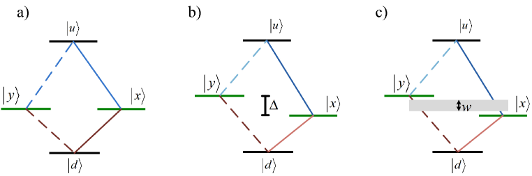
Figure 1: A decay cascade where the excited state, $\left|u\right\rangle$, decays to the ground state $\left|d\right\rangle$, along two decay paths each emitting two photons. The left (right) branch emits two photons that are vertically, $y$ (horizontally, $x$) polarized. In a) the intermediate level is degenerate and the cascade has perfect “which path ambiguity”. In b) the degeneracy of the intermediate level is slightly broken by the detuning $\Delta=|E_{x}-E_{y}|$. This cascade has “partial which path ambiguity”. c) shows how the entanglement can be distilled through spectral filtering by a window of width $w$ that erases the “which path” information

The two photons state, emitted by any one of the cascades in Fig. 1, is a pure entangled state. It is entangled because the quantum decay proceeds simultaneously along the two decay channels. This, however, does not imply that the associated pair of qubits, describing the state of polarization, are entangled. The state of the qubits is obtained from the quantum state of the photon field by tracing out all the degrees of freedom of the two photons (e.g. colors) save the polarization [8]. This state is in general, mixed, and possibly unentangled in contrast with the two photons state which is pure and entangled. In fact, partial path ambiguity caused by a detuning $\Delta$ that is large compared with radiative life times—normally the smallest energy scale in the problem—gives negligible entanglement of the two qubits. Fortunately, in this case, the entanglement can be distilled by erasing the “which path” information [9, 10] as indicated in Fig. 1 (c). In fact, by choosing a sufficiently narrow window, one can distill maximally entangled pairs. The price one pays is that the probability of finding close to maximally entangled pairs is then very small.

Decay cascades with “partial which-path ambiguity” are naturally found in the biexciton radiative cascade of semiconductor quantum dots [11, 12]. In these solid-state devices, there is an additional complication in that the energy levels of the cascade, are (correlated) random quantities that undergo slow (on the radiative time scale) fluctuations [13]. These arise from random variations in the electrostatic potential in the sample. The ensemble of photons emitted by the cascade is then a mixed state. Entanglement may or may not not be distilled in the case of general random cascades with large fluctuations. However, as we shall see, for a standard model of the random biexciton cascade, distillation works even when fluctuations are large [6].

Our theory allows one to compute the $4\times 4$ density matrix, $\rho$, of the two photon polarization from the spectral properties of the cascade. More precisely, we shall see that $\rho$, is determined by the quantum energies and life times of the energy levels in the cascade, their distribution, and the spectral width of the filter. All these quantities can either be measured or determined by the experimentalist. The theory avoids modelling the radiating system and we do not need to write a Hamiltonian for the radiating system. What we do need, instead, is a “universal” form for the photon state generated by a radiating (dipole) cascade. This 2-photon quantum state depends parameterically on the energies and lifetimes of the cascade. The theory applies irrespective of the nature of the source, be it a quantum dot, an atom, a molecule etc. It allows us to calculate the measure of entanglement [10] for a given cascade, with and without distillation. It also allows us to optimize the flux of entangled pairs.

The paper is organized as follows: In section 2 we describe the polarization density matrix for cascades with two decay channels. In section 3 we describe the state of the emitted photons from the radiative cascade in the dipole approximation. We describe the entanglement distillation in section 4 and the magnitude of the non-diagonal elements. In section 5 we discuss the phases of the non-diagonal elements of the density matrix. In section 6 we extend the theory to random cascades relevant to biexciton in quantum dots and in section 7 we compare our theory with the experimental results of Akopian et al. [6].

2 The polarization density matrix

Consider a radiating system, say a quantum dot, inside a micro-cavity followed by an appropriate optical setup for photon collection so that the outgoing radiation propagates along the positive $z$ axis. The polarization of the outgoing photons then lies in the $xy$ plane. The initial state of the system at time zero is an excited dot while the photon field is in its vacuum state, $\left|u\right\rangle\otimes\left|0\right\rangle$, see Fig. 1. For times much longer than the decay time of the dot, $1/\Gamma$, the dot is in the bottom state and the photon field has a pair of freely propagating photons, and the quantum state of the dot and photon filed is $\left|d\right\rangle\otimes\left|\psi\right\rangle$. Each decay path emits a pair of photons with a characteristic polarization: vertical polarization for the left path and horizontal for the right path [14]. The state of the freely propagating pair of photons is then necessarily of the form

$$\left|\psi(t)\right\rangle=\sum_{j=x,y}\int dk_{1}dk_{2}\,\lambda_{j}\,\alpha_{j}(k_{1},k_{2})e^{ic(|k_{1}|+|k_{2}|)t}\,{a^{{\dagger}}_{k_{1},{j}}a^{{\dagger}}_{k_{2},{j}}}\left|0\right\rangle\ .$$ (1)

$\lambda_{j}$ are the branching ratios for the two decay modes, $a^{{\dagger}}_{k,{j}}$ is a photon creation operator with wave vector $k$ and polarization $j$. Since $a^{{\dagger}}_{k_{1},{j}}a^{{\dagger}}_{k_{2},j}$ is symmetric in $k_{1}$ and $k_{2}$ only the symmetric part of the functions $\alpha_{j}(k_{1},k_{2})$ contributes to the integral reflecting the fact that photons are Bosons. We denote by $\alpha^{S}$ the symmetrization of $\alpha$ ,i.e.

$$\alpha^{S}(k_{1},k_{2})=\frac{\alpha(k_{1},k_{2})+\alpha(k_{2},k_{1})}{2}$$ (2)

Since the initial state was normalized and the evolution is unitary, so is the final state

$$\langle\psi(t)|\psi(t)\rangle=\sum_{j}|\lambda_{j}|^{2}\langle\alpha_{j}^{S}|\alpha_{j}^{S}\rangle=1,$$ (3)

We are interested in the correlations between the polarizations of two photons. This is fully described by the reduced polarization density matrix whose entries are given by [15]

$$\rho_{\mu,\nu;\mu^{\prime},\nu^{\prime}}=\sum_{k_{1},k_{2}}\left\langle\psi\right|a^{{\dagger}}_{k_{2},\nu}a^{{\dagger}}_{k_{1},\mu}a^{\phantom{{\dagger}}}_{k_{1},\nu^{\prime}}a^{\phantom{{\dagger}}}_{k_{2},\mu^{\prime}}\left|\psi\right\rangle$$ (4)

With $\left|\psi\right\rangle$ given by Eq. 1, one finds for $\rho$

$$\rho=\left(\begin{array}[]{cccc}|\lambda_{x}|^{2}&0&0&\gamma\\ 0&0&0&0\\ 0&0&0&0\\ \bar{\gamma}&0&0&|\lambda_{y}|^{2}\\ \end{array}\right),\quad\gamma=\lambda_{x}^{*}\lambda_{y}\langle\alpha_{x}^{S}|\alpha_{y}^{S}\rangle$$ (5)

in the basis $\left|xx\right\rangle$, $\left|xy\right\rangle$, $\left|yx\right\rangle$ and $\left|yy\right\rangle$ ($x$ and $y$ denote the state of polarization). This special form expresses the fact that the amplitude for all processes involving the polarization states $\left|xy\right\rangle$ and $\left|yx\right\rangle$ vanish. Note that the matrix has normalized trace, $|\gamma|\leq\mbox{$\frac{1}{2}$}$ and that the state is mixed for $|\langle\alpha_{x}|\alpha_{y}\rangle|<1$.

The two qubits are maximally entangled when $|\lambda_{j}|^{2}=|\gamma|=\mbox{$\frac{1}{2}$}$. When $\gamma=0$ the polarization state is separable and may be thought of as a classical random source of correlated qubits. $|\gamma|$ is a measure of the entanglement known as the negativity [16, 17], (being the negative eigenvalue of the partial transposition of $\rho$.)

In the following sections we describe a theory that allows us to compute $\gamma$ as a function of the spectral properties of the cascade.

3 Photons in the dipole approximation

To make progress we need to know the functions $\alpha_{j}$ of Eq. (1). For this we need to make some assumptions about the nature of the radiating system. Consider sources that are small compared with the wavelength of the radiation they emit. For such sources the dipole approximation applies. We shall further assume that the interaction between the source and radiation field is weak so that the rotating wave approximation applies [18]. In this setting, which applies to a wide varieties of radiating systems, the function $\alpha_{j}$ can be calculated explicitly. For a radiative cascade with a single branch this function is given e.g. in [18, 19]. The case of two branches is then simply a weighted superposition, as in Eq. (1).

For each branch the function $\alpha_{j}$ can be expressed in terms of the spectral properties of the cascade: $Z_{\ell}=E_{\ell}-i\Gamma_{\ell},\ \ell=x,y,u$. $E_{\ell}$ is the energy of the $\ell$-th state (we chose the ground state to have zero energy, $E_{d}=0$) and $\Gamma_{\ell}$ is its width. For a dipole at the origin one has [19]:

$$\alpha_{j}(k_{1},k_{2})=A(k_{2},Z_{j})\,A(k_{1}+k_{2},Z_{u})$$ (6)

where

$$A(k,Z)=\frac{\sqrt{\Gamma/\pi}}{|k|-Z},\quad Z=E-i\Gamma$$ (7)

and we use units where $\hbar=c=1$. This reduces the problem of computing the entanglement $\gamma$ of Eq. (5) to computing integrals.

3.1 The limit of small radiative width

In most applications, the radiative widths $\Gamma_{\ell}$ are the smallest energy scale in the problem. This is the case for the biexciton decay in quantum dot where $\Gamma_{\ell}\sim 0.8\mu\,eV)$, the detuning $\Delta=|E_{x}-E_{y}|\sim 27\mu\,eV)$ and the energies of the emitted photons are much larger [20], $E_{\ell}-E_{\ell^{\prime}}\sim 1.32\,eV)$.

The smallness of $\Gamma$ leads to simplifications in many of the integrals which can then be evaluated analytically. For example, $A(k,Z)$ is concentrated near $E$ with a width $\Gamma$, so, in the limit that $\Gamma$ is small, one makes only a small error by replacing $|k|$ by $k$. It then follows that, to leading order in $\Gamma/E$

$$\langle A|A\rangle=\int dk|A|^{2}\approx\frac{\Gamma}{\pi}\int\frac{dk}{(k-E)^{2}+\Gamma^{2}}=1$$ (8)

In general, as in the case of biexciton decay, the two photons emitted in each cascade have different colors, namely,

$$\Gamma\ll|(E_{u}-E_{j})-(E_{j}-E_{d})|$$ (9)

This distinguishes the two photons which may therefore be treated as distinct particles and one may forget about the symmetrization, Eq. (2). Mathematically, this follows from the observation that in computing overlaps, products of the form

$$A(k_{1},Z_{j})A^{*}(k_{2},Z_{j})|A(k_{1}+k_{2},Z_{u})|^{2}$$ (10)

are small and can be neglected.

This allows us to immediately show that the entanglement in a cascade with partial which path ambiguity is negligible when $\Delta\gg\Gamma$. This follows from

$${\langle\alpha_{x}^{S}|\alpha_{y}^{S}\rangle}\approx{\langle\alpha_{x}|\alpha_{y}\rangle}\approx\left(\frac{\Gamma^{2}}{\Delta^{2}+\Gamma^{2}}\right)^{\mbox{$\frac{1}{2}$}}\approx\frac{\Gamma}{\Delta}$$ (11)

The different colors of the emitted photons resolve the “which path ambiguity”. This mixes the two qubits and essentially kills the entanglement.

4 Entanglement distillation

The entanglement can be distilled by selecting those photons which does not betray the decay path [6]. Let us denote the average intermediate states (exciton) energy as $2\bar{E}=E_{x}+E_{y}$. The first emitted photon do not betray the decay path provided one only looks at energies near $E_{u}-\bar{E}$. Similarly, the second photon does not betray the decay path provided one only collects photons with energies $\bar{E}$.

In practice, the distillation is done by filtering the photons through a spectral window function. The photons are detected only if their energy is either within a window of width $w$ centered at $E_{u}-\bar{E}$ or within one centered at $\bar{E}$. This is implemented by a monochromator (an energy filter) which transmits only a selected part of the emission spectrum [6].

Most photon pairs, are of course, lost in the distillation process. Roughly, the fraction of photon pairs that are filtered is of the order $O(w/\Delta)$, as most photons lie in the window of width $\Delta+O(\Gamma)$. One might worry that, to be effective, the window must be of the order of the radiative life-time, $w=O(\Gamma)$. If that was the case, only a very small fraction of the photon pairs could be distilled. As we shall see, however, this is not the case. In fact, one may choose $w=O(\Delta)$ so a substantial fraction of the photons will be distilled while obtaining considerable entanglement. The price one pays for filtering is that the source is not “on demand” but rather a random source of entangled photons [6].

The filtering process is represented in the theory by a projection operator $W$, which eliminates from a Fock state all photons spare those whose energy lies within appropriate energy windows (irrespective of polarization). Here we are only interested in the two photon component of the state after filtration. Therefore, one can effectively express the action of the operator $W$ as

$$W:\alpha_{j}(k_{1},k_{2})\to w(k_{1})w(k_{2})\alpha_{j}(k_{1},k_{2})$$ (12)

where $w(k)$ is the step function

$$w(k)=\left\{\begin{array}[]{ll}1&|k-(E_{u}-\bar{E})|<w/2\\ 1&|k-\bar{E}|<w/2\\ 0&{\rm otherwise\par}\end{array}\right.$$ (13)

Evidently, $W$ is a projection operator, i.e. $W^{2}=W$. The identity $W=1$ ($w=\infty$) represents no filtering.

The distillation succeeds with probability $p_{W}={\left\langle\psi\right|W\left|\psi\right\rangle}$ and produces the (normalized) filtered state

$$\left|\psi^{f}\right\rangle=\frac{W\left|\psi\right\rangle}{\sqrt{p_{W}}}$$ (14)

The filtered, or distilled, density matrix can be computed from the distilled state. In particular, for the entanglement, as measured by $\gamma$ of Eq. (5) we find

$$\gamma_{d}=\lambda^{*}_{x}\lambda_{y}\frac{\left\langle\alpha_{x}^{S}\right|W\left|\alpha_{y}^{S}\right\rangle}{p_{W}},\quad p_{W}=\sum_{j=x,y}|\lambda_{j}|^{2}\left\langle\alpha_{j}^{S}\right|W\left|\alpha_{j}^{S}\right\rangle$$ (15)

This reduces the problem to computing integrals, where we account for $W$ by summing only the appropriate wavevectors. Fig. 2 shows the probability to detect a pair of photons and $\gamma_{d}$ of the distilled state, as function of the width of the spectral window $w$. To plot the figure we use parameter values corresponding to biexciton decay in a quantum dot. As one expects, the entanglement is a decreasing function of $w$, (for a window of zero width one gets a maximally entangled state). On the other hand, the probability that the detection succeeds is, of course, an increasing function of the width.

Figure 2: The probability that distillation succeeds is an increasing function of the window $w$ shown in the red dotted curve. The entanglement of the distilled pair is a decreasing function of $w$ shown in the blue curve. The pair is maximally entangled at $w=0$. The plot is drawn for parameter values corresponding to biexciton decay where $\Delta/\Gamma\approx 17$.

The qualitative behavior of entanglement distillation can be gleaned by inspection of Fig. 3. The function $\alpha_{x}$ is concentrated in a small neighborhood of size $O(\Gamma)$ near the point of intersection of the green and blue curve. Similarly, $\alpha_{y}$ is concentrated near the intersection of the purple and blue curve. For example, the fact that the entanglement without distillation is small, Eq. (11), follows from the little overlap of $\langle\alpha_{x}|\alpha_{y}\rangle$ each of which is concentrated near a different point. Due to distillation, only amplitudes contained in the intersection of red squares are collected. This does two things. It decreases the numerator in Eq. (15) which is bad. However, it also decreases the denominator which is good. This decrease is much more significant and consequently the entanglement increases.

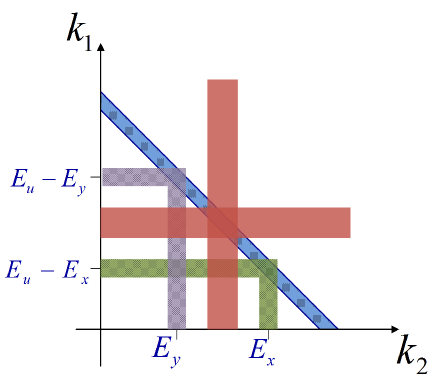
Figure 3: The wave function $\alpha_{x}$ is large near the intersection of the diagonal strip, expressing total energy conservation, with the line which represents the $x$ decay path where the second photons has energy $E_{x}$. Similarly, the function $\alpha_{y}$ is large near the intersection of the diagonal strip with the line representing the $y$ decay path where the second photon has energy $E_{y}$. The cross represents a filter of narrow width. The filter collects photons that are contained in the intersection of the cross.

Perhaps the most interesting things one learns form Fig. 3 is how wide does a window have to be to betray the “which path information”. This happens when the window contains the points of intersections, either red with purple, or red with green. If the window does not contain these points the path is not betrayed. Since the points have a small size, $O(\Gamma)$, this implies that the size of the optimal window is of the scale of the detuning, $w=\Delta-O(\Gamma)$. Because this window is not small, the probability that the distillation succeeds is not very small either.

5 The phase problem

From the perspective of quantum information theory the phases in the density matrix are gauge dependent quantities (as they are not invariant under local unitary operations [21]). Even if Alice and Bob fix the projectors $\left|0\right\rangle\left\langle 0\right|$ and $\left|1\right\rangle\left\langle 1\right|$, there is still a freedom to choose the phases of the states

$$\left|a\right\rangle\otimes\left|b\right\rangle\to e^{i\phi_{a}}e^{i\varphi_{b}}\left|a\right\rangle\otimes\left|b\right\rangle,\quad a,b\in\{0,1\}.$$ (16)

We refer to this as gauge freedom. Such a transformation will change the phases of the non-diagonal entries of the density matrix

$$\rho_{ab,cd}\to e^{i(\phi_{a}+\varphi_{b}-\phi_{c}-\varphi_{d})}\rho_{ab,cd},\quad a,b,c,d\in\{0,1\}$$ (17)

in the computational basis. Any reasonable measure of entanglement, and in particular $|\gamma|$ of Eq. (5), is clearly independent of the choice of gauge.

Quantum tomography [22] is an algorithm to convert 16 measurements to the 16 (complex) entries of the density matrix $\rho$ (describing the ensemble) [23]. This means that any quantum tomography algorithm must fix both the projectors representing the “computational” basis and fix the gauge.

In the context of photon polarization the canonical choice (which we used throughout this paper) of the “computational” basis is the projectors associated with the $x$ and $y$ linear polarizations. The remaining gauge freedom is

$$a_{kj}\to e^{i\phi_{j}}a_{kj},\quad a_{kj}^{\dagger}\to e^{-i\phi_{j}}a_{kj}^{\dagger}\qquad j=x,y$$ (18)

for two orthogonal polarizations $j$. Fixing the right circular polarization by

$$a_{k,R}^{\dagger}=\frac{a_{kx}^{\dagger}+ia_{ky}^{\dagger}}{\sqrt{2}}$$ (19)

fixes the gauge since

$$a_{kR}\to e^{i\phi_{R}}a_{kR},\quad a_{kR}^{\dagger}\to e^{-i\phi_{R}}a_{kR}^{\dagger}\,,$$ (20)

requires that all the $\phi$’s are the same. This then fixes the phase of $\gamma$.

The phase of $\gamma$, which was measured in [6, 24, 25] have, so far, not been explained by a theoretical model. In the following, we calculate this phase and describe the physical information that is encoded in it.

Eq. (15) determines $\gamma$ in terms of the product of the branching ratios $\lambda_{x}\lambda^{*}_{y}$ and the overlap $\left\langle\alpha_{x}^{S}\right|W\left|\alpha_{y}^{S}\right\rangle$. In the next section, we shall show that for a decay cascade with partial which path ambiguity and time-reversal invariance, $\lambda_{x}\lambda^{*}_{y}>0$. It then follows that the phase of $\gamma$ is fully determined by the phase of $\left\langle\alpha_{x}^{S}\right|W\left|\alpha_{y}^{S}\right\rangle$.

5.1 Branching ratios

The branching amplitudes $\lambda_{j}$ of Eq. (1) are proportional to the appropriate dipole matrix elements

$$\lambda_{x} = \zeta\left\langle u\right|X\left|j\right\rangle\left\langle j\right|X\left|d\right\rangle$$

$$\lambda_{y} = \zeta\left\langle u\right|Y\left|j\right\rangle\left\langle j\right|Y\left|d\right\rangle$$ (21)

where $\zeta$ is a overall normalization constant and $X$ is the x component of the (possibly multi-electron) position operator and similarly $Y$ is the y component of the position operator. It follows that

$$\lambda_{x}^{*}\lambda_{y}=|\zeta|^{2}\,\left\langle d\right|X\left|x\right\rangle\left\langle x\right|X\left|u\right\rangle\left\langle u\right|Y\left|y\right\rangle\left\langle y\right|Y\left|d\right\rangle$$ (22)

Observe first, that this quantity is independent of the gauge choice of the states $\left|\ell\right\rangle$ of the source, as every ket is paired with the corresponding bra. We shall now show that in the case that all the states $\left|\ell\right\rangle$ are non-degenerate, there is a choice of gauge so that each matrix element in the product is real.

Let $T$ denote the antiunitary operator associated with time reversal [26, 27], i.e.

$$\langle T\ell|Tk\rangle=\langle k|\ell\rangle$$ (23)

In the case that all states $\left|\ell\right\rangle$ are non-degenerate $T\left|\ell\right\rangle=e^{i\beta_{\ell}}\left|\ell\right\rangle$. By changing the gauge to $\left|\ell\right\rangle\to e^{i\beta_{\ell}/2}\left|\ell\right\rangle$, one sees that $\left|\ell\right\rangle$ may be chosen so that $T\left|\ell\right\rangle=\left|\ell\right\rangle$. The position operator is evidently even under time reversal e.g. $T^{*}XT=X$. Plugging this in the definition of the dipole matrix elements we see that

$$\left\langle\ell\right|X\left|k\right\rangle=\left\langle\ell\right|T^{*}XT\left|k\right\rangle=\left\langle T\ell\right|X\left|Tk\right\rangle=\left\langle k\right|X\left|\ell\right\rangle$$ (24)

We have therefore shown that $\lambda_{x}^{*}\lambda_{y}$ is a real number. We shall now show that under rather weak continuity assumptions, it must actually be positive. $\lambda_{x}^{*}\lambda_{y}$ is a function of the spectral properties of the cascade, and in particular, it is a function of the detuning $\Delta$. It has the same sign as $\Delta$ varies so long as the two decay paths are indeed effective (none of the branching ratios, $\lambda_{j}$, vanishes). It is therefore enough to determine the sign at a single point. We shall now give a symmetry argument that at $\Delta=0$ one has $\lambda_{x}^{*}\lambda_{y}>0$.

Assume that the degeneracy $\Delta=0$ is a consequence of (possibly approximate) rotational symmetry in the x-y plane of the radiating system, (this is the case in quantum dots). Since the sign of the product of dipole matrix elements changes continuously as the Hamiltonian is deformed, we may compute the sign for the case where the rotational symmetry is exact. In this case, as the initial, non-degenerate, state $\left|u\right\rangle$ must be a state of angular momentum 0 about the z-axis. Since angular momentum is conserved the final two photon state must also be a state of zero angular momentum about the z-axis.

In this case, perfect which path ambiguity and zero angular momentum imply that the state of the outgoing photons is

$$\left|\psi(t)\right\rangle=\int\frac{dk_{1}dk_{2}}{\sqrt{2}}\,\alpha(k_{1},k_{2})e^{i(|k_{1}|+|k_{2}|)t}\,\left(a^{{\dagger}}_{k_{1},R}a^{{\dagger}}_{k_{2},L}+a^{{\dagger}}_{k_{1},L}a^{{\dagger}}_{k_{2},R}\right)\left|0\right\rangle,$$ (25)

By comparing this with Eq. 1 one easily sees that this state implies $\lambda_{j}=1/\sqrt{2}$. Hence, $\gamma=\mbox{$\frac{1}{2}$}$ in Eq. (5), which determines the sign of the product $\lambda_{x}^{*}\lambda_{y}>0$.

5.2 The role of the complex pole

It follows from the analysis above that the phase of $\gamma$ is the same as the phase of $\left\langle\alpha_{x}\right|W\left|\alpha_{y}\right\rangle$. The latter is determined by a two-dimensional integration of the function

$$w(k_{1})w(k_{2})\ \Big{|}A(k_{1}+k_{2},Z_{u})\Big{|}^{2}\,A(k_{2},Z_{j})\bar{A}(k_{2},Z_{j^{\prime}})$$ (26)

The first three factors are positive, and weigh the integrand. The third factor may be interpreted as guaranteeing approximate conservation of total energy since

$$\lim_{\Gamma\to 0}\Big{|}A(k,Z)\Big{|}^{2}=\delta(|k|-E)$$ (27)

This means that to leading order in $\Gamma$ the matrix elements of $\rho$ are determined by a one-dimensional integral over $k$ of the function

$$w(E_{u}-k)w(k)\ A(k,Z_{j})\bar{A}(k,Z_{j^{\prime}})$$ (28)

The phase of $\gamma$ is governed by the phase of $A(k,Z_{x})A^{*}(k,Z_{y})$ which is represented graphically in Fig. 4

Strong filtering:

Suppose the filtering window $W$ is very narrow with width $\Gamma<w\ll\Delta$. The window restricts the domain of integration to a very narrow region. The detection probability is small and scales linearly with the window’s width $p_{W}=O(\frac{w\Gamma}{\Delta^{2}})$. The phase of $\gamma$ is $\pi-4\Gamma/\Delta$ and the magnitude is approximately.

$$\gamma=-\mbox{$\frac{1}{2}$}+O\left(\frac{\Gamma}{\Delta}\right)$$ (29)

The state is close to a maximally entangled state. This gives the upper left triangle of Fig. 5 and the left part of Fig. 2.

No filtering:

No filtering corresponds to $W=1$ and a width $w=\infty$. Exact degeneracy, $\Delta=0$, gives a maximally entangled state, $\gamma=1/2$. (The two arrows in Fig. 4 are complex conjugates.)

When $\Delta\gg\Gamma$ the integrals are dominated by the neighborhood of the poles at $k=E_{x},E_{y}$. The off-diagonal element is almost purely imaginary and $\gamma=O\left(i\frac{\Gamma}{\bar{\Delta}}\right)$. This accounts for the lower right hand triangle of Fig. 5 and the right hand part of Fig. 2.

(a)

(b)

(c)

Figure 4: The phase is determined by the product of the two complex numbers $(k-Z_{x})(k-Z_{y}^{*})$. The numbers are represented as arrows pointing from $k$ to the location of the complex energies $Z_{\varepsilon}$ (blue arrow for $Z_{x}$ and red arrow for $Z_{y}$). The location of $k$ is restricted by the window function $W$. In figure (a) the levels are detuned and the spectral window is smaller than the detuning. In figure (b) the levels are degenerate and in figure (c) the levels are detuned and the window is larger than the detuning.

Figure 5: The phase of $\gamma$ as a function of the (centered) normalized spectral window width $w/\Gamma$ and the detuning $\Delta/\Gamma$ for parameters appropriate to biexciton in a quantum dot. The triangular reagin above the diagonal represents the situation of a narrow filter where $\gamma\sim-1/2$. The triangular region below the diagonal is where the window is large, $\gamma$ is small and essentially purely imaginary. At the bottom of the figure the detuning is small and $\gamma\sim 1/2$.

6 Random cascades

Radiative cascades with partial which path ambiguity are found naturally in semiconductor quantum dots where $\left|u\right\rangle$ is the ground state of a bound state of a pair of two electrons and two holes (a biexciton). The states $|x\rangle$ and $|y\rangle$ are the ground and first excited state of the bright exciton (a bound electron-hole pair). The state $|d\rangle$ describes an empty quantum dot. In this case the energies and states slowly fluctuate due to electrostatic transients in the semiconductor hosting the quantum dots. In typical cases [6], the fluctuations are large (comparable to $\Delta$) and slow (the time scale is much longer than $1/\Gamma$).

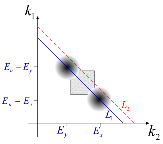
Figure 6: The gray shapes represent the fluctuations of the cascade. The lines diagonal represent conservation of total energy and correlate the two gray shapes. They fluctuate as well. The rectangle represents the filtering. In a) some of the events penetrate the filter and thus betray the which path ambiguity. In b) the fluctuations do not betray the which path ambiguity and entanglement can be filtered.

One can model the situation by letting the spectral properties of the cascades, namely $Z_{\ell}(s)$, be appropriate functions of a random variables $s$, with measure $dP(s)$. The two-photon state of Eq. (1), $\left|\psi(s)\right\rangle$ is then a random variable.

The photon field $\left|\psi(s)\right\rangle$ of Eq. (1), depends on $s$ through the fluctuating complex energies, $Z_{\ell}$, of Eq. (6). The 2 photon state emitted by the dot is then described not by a pure state but rather by a density matrix

$$\rho_{r}=\int dP(s)\left|\psi(s)\right\rangle\left\langle\psi(s)\right|.$$ (30)

The probability to distill a state describing a specific random event is

$$p(s)=\left\langle\psi(s)\right|W\left|\psi(s)\right\rangle.$$ (31)

Therefore, the probability to distill a photon pair is given by

$$p(W|\rho_{r})=\int p(s)P(s)ds$$ (32)

Similarly, the value of the distilled $\gamma_{d}$ is given by averaging over $s$

$$\gamma_{d}=\frac{\int dP(s)\,p(s)\,\gamma_{d}(s)}{\int dP(s)p(s)}$$ (33)

where $\gamma(s)$ is given by substituting $\left|\psi(s)\right\rangle$ in Eq. (15).

In general, large spectral fluctuations can potentially destroy the distillation based on fixed spectral windows. This, for example, is the situation when the values of $E_{u},E_{x}$ and $E_{y}$ are independent random variables, as illustrated in Fig. 6(a). In the figure, the amplitudes which betray the which path ambiguity penetrate the filter. When the fluctuations are smaller than $\Delta$ one can remedy this by choosing a sufficiently small spectral window. This situation is illustrated in Fig. 6(a). However, when the fluctuations are larger than $\Delta$ distillation becomes impossible.

A scenario which allows for distillation also when the fluctuations are larger than $\Delta$ is illustrated in Fig. 6(b).

At first, one may think that the second “good” scenario is contrived and would not naturally occur. In fact, this is not the case and this scenario is the one that describes biexciton drift. The reason is that the energies $E_{u}$, $E_{y}$ and $E_{x}$ are not independent random variables, as in Fig. 6(a), but rather dependent random variables. This is because for a biexciton, $E_{u}=E_{x}+E_{y}-B$ where $B$ is the biexciton binding energy [28] which is typically more than two orders of magnitude smaller than the exciton energy and its dependence on $s$ can be safely ignored. A model for a fluctuating spectral diagram is then

$$E_{x}\to E_{x}+s,\quad E_{y}\to E_{y}+s,\quad E_{u}\to E_{u}+2s$$ (34)

This indeed leads to a scenario like the one illustrated in Fig 6(b).

We note that the biexciton drift described above has only little effect on the calculation of $\gamma_{d}$ described in section 5 and Fig 5. This results from the rapid decrease of the probability of detection $p(s)$ from its maximal value at $s=0$. This can be seen in Fig. 7 which plots $p(s)dP(s)$ for finite value of $\Gamma$.

Figure 7: The relative “weight” of the density matrix $\rho(s)$. The weight is given by $\Lambda(s)=P(s)Tr(W\rho(s))$. The plot is renormalized to yield $\Lambda(0)=1$. The plot is obtained with the experimental values as in Sec. 7.

7 Comparison with experiment

We now turn to compare the theoretical calculation with the experimental data as described by Akopian et al. [6]

The parameters used in the theory were measured independently: $\Gamma_{x}\approx\Gamma_{y}=0.8\pm 0.2[\mu eV],\ \Gamma_{u}\approx 2\Gamma_{x}$ and $E_{x}\approx E_{y}=1.28[eV],\ E_{u}=2.55[eV]$, $\Delta=27\pm 3[\mu eV]$. The window that was used in the experiment was of width $w=25\pm 10[\mu eV]$.

The distribution $P(s)$ of the spectral shift was evaluated from the measured spectral lines. It was rather wide, with full width middle height of about $50[\mu eV]$. With the values listed above the probability of detection $Tr(W\rho(s))$ falls much faster then the distribution $P(s)$ as a function of $|s|$, to half its value at $|s|\sim 5\Gamma\sim 8[\mu eV]$.

The numerically calculated contribution to the filtered state (i.e. probability of detection times probability distribution for $s$) as a function of the spectral drift $s$ for the above parameters is displayed in Fig. 7.

When we come to compare the theory with the experimental results, we must take into account the measurement error of the tomography, as well as the errors on the parameters $\Delta,\Gamma$,$s$ and $w$ (the QD or model parameters). These are displayed in Fig. 8. The measured phase in the experiment was $-110^{\circ}\pm 17^{\circ}$ where we have taken into account the effect of the beam splitter. The beam splitter induces a phase shift of $180^{\circ}$ between the X and Y polarizations of the reflected photon only (this was ignored in Akopian et al. [6], where the phase was reported $70^{\circ}$). This is compared to the theoretical result $-160^{\circ}\pm 45^{\circ}$, which shows a reasonable fit with the experiment.

Figure 8: Comparison between the experimental results of Akopian et al. and the theory. The graph shows a theoretical calculation of the phase as a function of the window, $w$ and the detuning, $\Delta$, both in units of $\Gamma$. The calculation uses the experimentally measured parameters $w$, $\Delta$, $\Gamma$ and $s_{0}$. The uncertanties in these parameters result in an area (rather than a point) indicated by the error bars. The possible theoretical values of the phase are in the area which is bounded by these error bars. This values are compared to the experimentally measured phase and error, which is represented in the color bar to the left.

8 Conclusion

We described a framework to calculate the density matrix of a pair of photons emitted in a decay cascade with partial which path ambiguity, encoded in the energies of the emitted photons. We showed that one can distill the entanglement by selecting only the photons possessing ”which path” ambiguity and discuss how this distillation by spectral filtering affect the phase of the non-diagonal elements of the two photon density matrix. We showed that spectral filtering is quite robust and protected from fluctuations in the level’s energies as long as these fluctuations are correlated. Our calculations, quantitatively describe measurements performed on semiconductor quantum dots.

References

- [1] Charles H. Bennett and David P. DiVincenzo. Quantum information and computation. Nature, 404:247–255, 2000.
- [2] N. Gisin, G. Ribordy, W. Tittel, and H. Zbinden. Quantum cryptography. Reviews of Modern Physics, 74:145–195, January 2002.
- [3] K. Mattle, H. Weinfurter, P. G. Kwiat, and A. Zeilinger. Dense Coding in Experimental Quantum Communication. Physical Review Letters, 76:4656–4659, June 1996.
- [4] D. Bouwmeester, J.-W. Pan, K. Mattle, M. Eibl, H. Weinfurter, and A. Zeilinger. Experimental quantum teleportation. Nature, 390:575–579, December 1997.
- [5] L. M. K. Vandersypen, M. Steffen, G. Breyta, C. S. Yannoni, M. H. Sherwood, and I. L. Chuang. Experimental realization of Shor’s quantum factoring algorithm using nuclear magnetic resonance. Nature, 414:883–887, December 2001.
- [6] N. Akopian, N. H. Lindner, E. Poem, Y. Berlatzky, J. Avron, D. Gershoni, B. D. Gerardot, and P. M. Petroff. Entangled photon pairs from semiconductor quantum dots. Physical Review Letters, 96(13):130501, 2006.
- [7] O. Benson, C. Santori, M. Pelton, and Y. Yamamoto. Regulated and Entangled Photons from a Single Quantum Dot. Physical Review Letters, 84:2513–2516, March 2000.
- [8] A. Peres. Quantum mechanics: Concepts and Methods. Kluwer, 1995.
- [9] T. J. Herzog, P. G. Kwiat, H. Weinfurter, and A. Zeilinger. Complementarity and the Quantum Eraser. Physical Review Letters, 75:3034–3037, October 1995.
- [10] R. Horodecki, P. Horodecki, M. Horodecki, and K. Horodecki. Quantum entanglement. ArXiv:quant-ph/0702225, February 2007.
- [11] T. Takagahara. Effects of dielectric confinement and electron-hole exchange interaction on excitonic states in semiconductor quantum dots. Phys. Rev. B, 47(8):4569–4584, Feb 1993.
- [12] M. Bayer, A. Kuther, A. Forchel, A. Gorbunov, V. B. Timofeev, F. Schäfer, J. P. Reithmaier, T. L. Reinecke, and S. N. Walck. Electron and hole factors and exchange interaction from studies of the exciton fine structure in quantum dots. Phys. Rev. Lett., 82(8):1748–1751, Feb 1999.
- [13] S. A. Empedocles, D. J. Norris, and M. G. Bawendi. Photoluminescence spectroscopy of single cdse nanocrystallite quantum dots. Phys. Rev. Lett., 77(18):3873–3876, Oct 1996.
- [14] F. Troiani, J. I. Perea, and C. Tejedor. Cavity-assisted generation of entangled photon pairs by a quantum-dot cascade decay. Phys. Rev. B, 74(23):235310–+, December 2006.
- [15] L. Mandel and E. Wolf. Optical coherence and quantum optics. Cambridge: Cambridge University Press, 1995.
- [16] Asher Peres. Separability criterion for density matrices. Phys. Rev. Lett., 77(8):1413–1415, Aug 1996.
- [17] Horodecki R. Violating bell inequality by mixed spin-1/2 states: necessary and sufficient condition. Physics Letters A, 200:340–344(5), 1 May 1995.
- [18] M. O. Scully and M. S. Zubairy. Quantum Optics. Cambridge University Press, 1997.
- [19] J. Dupont-Roc C. Cohen-Tannoudji and G. Grynberg. Atom-Photon Interactions. John Wiley & Sons, 1992.
- [20] E. L. PIvchenko and Grigorii E. Pikus. Superlattices and other heterostructures : symmetry and optical phenomena. Springer, 2nd ed. edition, 1997.
- [21] Charles H. Bennett, Herbert J. Bernstein, Sandu Popescu, and Benjamin Schumacher. Concentrating partial entanglement by local operations. Phys. Rev. A, 53(4):2046–2052, Apr 1996.
- [22] Daniel F. V. James, Paul G. Kwiat, William J. Munro, and Andrew G. White. Measurement of qubits. Phys. Rev. A, 64(5):052312, Oct 2001.
- [23] G. M. D’Ariano, L. Maccone, and M. G. A. Paris. Orthogonality relations in quantum tomography. Physics Letters A, 276:25–30, October 2000.
- [24] K. Edamatsu, G. Oohata, R. Shimizu, and T. Itoh. Generation of ultraviolet entangled photons in a semiconductor. Nature, 431:167–170, September 2004.
- [25] Young et. al. Improved fidelity of triggered entangled photons from single quantum dots. NJP, 8(29), Feburary 2006.
- [26] Robert G. Sachs. The physics of time reversal. University of Chicago Press, 1987.
- [27] Albert Messiah. Quantum mechanics. Amsterdam, 1961.
- [28] S. Rodt, A. Schliwa, K. Pötschke, F. Guffarth, and D. Bimberg. Correlation of structural and few-particle properties of self-organized InAs/GaAs quantum dots. Phys. Rev. B, 71(15):155325–+, April 2005.