Secrecy Capacity Region of Fading Broadcast Channels

Abstract

The fading broadcast channel with confidential messages (BCC) is investigated, where a source node has common information for two receivers (receivers 1 and 2), and has confidential information intended only for receiver 1. The confidential information needs to be kept as secret as possible from receiver 2. The broadcast channel from the source node to receivers 1 and 2 is corrupted by multiplicative fading gain coefficients in addition to additive Gaussian noise terms. The channel state information (CSI) is assumed to be known at both the transmitter and the receivers. The secrecy capacity region is first established for the parallel Gaussian BCC, and the optimal source power allocations that achieve the boundary of the secrecy capacity region are derived. In particular, the secrecy capacity region is established for the Gaussian case of the Csisz$\acute{\text{a}}$r-K$\ddot{\text{o}}$rner BCC model. The secrecy capacity results are then applied to give the ergodic secrecy capacity region for the fading BCC.

I Introduction

The wire-tap channel models a communication system in which a source node wishes to transmit confidential information to a destination node and wishes to keep a wire-tapper as ignorant of this information as possible. This channel was introduced by Wyner in [1], where the secrecy capacity was given. The secrecy capacity of the Gaussian wire-tap channel was given in [2]. The wire-tap channel was considered recently for fading and multiple antenna channels in [3, 4]. A more general model of the wire-tap channel was studied by Csisz$\acute{\text{a}}$r and K$\ddot{\text{o}}$rner in [5], where the source node also has a common message for both receivers in addition to the confidential message for only one receiver. This channel is regarded as the broadcast channel with confidential messages (BCC). The capacity-equivocation region and the secrecy capacity region of the discrete memoryless BCC were characterized in [5]. The BCC was further studied recently in [6], where the source node transmits two confidential message sets for two receivers, respectively.

In this paper, we investigate the fading BCC, which is based on the BCC studied in [5] with the channels from the source node to receivers 1 and 2 corrupted by multiplicative fading gain coefficients in addition to additive Gaussian noise terms. We assume that the channel state information (CSI) is known at both the transmitter and the receivers. The CSI at the transmitter (the source node) can be realized by reliable feedback from the two receivers, who are supposed to receive information from the source node.

The fading BCC we study in this paper relates to or generalizes a few channels that have been previously studied in the literature. Compared to the fading broadcast channel studied in [7, 8, 9, 10, 11], the fading BCC requires a secrecy constraint that the confidential information for one receiver must be as secret as possible from the other receiver. The fading BCC includes the fading wire-tap channel studied in [12, 13] and [14] (full CSI case) as a special case, because the fading BCC assumes that the source node has a common message for both receivers in addition to the confidential message for receiver 1. The fading BCC also includes the parallel Gaussian wire-tap channel studied in [15] (the case where wire-tappers cooperate) as a special case for the same reason as above and also because a power constraint is assumed for each subchannel in [15].

In this paper, we first study the parallel Gaussian BCC, which serves as a basic model that includes the fading BCC as a special case. We show that the secrecy capacity region of the parallel Gaussian BCC is a union over the rate regions achieved by all source power allocations (among the parallel subchannels). Moreover, we derive the optimal power allocations that achieve the boundary of the secrecy capacity region and hence completely characterize this region. In particular, we establish the secrecy capacity region of the Gaussian case of the Csisz$\acute{\text{a}}$r-K$\ddot{\text{o}}$rner BCC model.

We then apply our results to study the fading BCC, which can be viewed as the parallel Gaussian BCC with each fading state corresponding to one subchannel. Thus, the secrecy capacity region of the parallel Gaussian BCC applies to the fading BCC. In particular, since the source node knows the CSI, it can dynamically change its transmission power with channel state realization to achieve the boundary of the secrecy capacity region.

In this paper, we use $X_{[1,L]}$ to indicate a group of variables $(X_{1},X_{2},\ldots,X_{L})$, and use $X_{[1,L]}^{n}$ to indicate a group of vectors $(X_{1}^{n},X_{2}^{n},\ldots,X_{L}^{n})$, where $X_{l}^{n}$ indicates the vector $(X_{l1},X_{l2},\ldots,X_{ln})$. Throughout the paper, the logarithmic function is to the base $2$.

The paper is organized as follows. We first study the parallel Gaussian BCC. We then study the fading BCC and demonstrate our results with numerical examples. We conclude the paper with a few remarks.

II Parallel Gaussian BCCs

We consider the parallel Gaussian BCC with $L$ independent subchannels (see Fig. 1), where there are one source node and two receivers. As in the BCC, the source node wants to transmit common information to both receivers and confidential information to receiver 1. Moreover, the source node wishes to keep the confidential information to be as secret as possible from receiver 2.

For each subchannel, outputs at receivers 1 and 2 are corrupted by additive Gaussian noise terms. The channel input-output relationship is given by

$$Y_{li}=X_{li}+W_{li},\hskip 14.22636ptZ_{li}=X_{li}+V_{li},\hskip 14.22636pt\text{for }\;l=1,\ldots,L$$ (1)

where $i$ is the time index. For $l=1,\ldots,L$, the noise processes $\{W_{li}\}$ and $\{V_{li}\}$ are independent identically distributed (i.i.d.) with the components being Gaussian random variables with the variances $\mu_{l}^{2}$ and $\nu_{l}^{2}$, respectively. We assume $\mu_{l}^{2}<\nu_{l}^{2}$ for $l\in A$ and $\mu_{l}^{2}\geq\nu_{l}^{2}$ for $l\in A^{c}$. The channel input sequence $X_{[1,L]}^{n}$ is subject to the average power constraints $P$, i.e.,

$$\frac{1}{n}\sum_{i=1}^{n}\sum_{l=1}^{L}\mathrm{E}\left[X_{li}^{2}\right]\leq P.$$ (2)

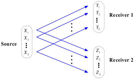
Figure 1: Parallel BCC

A $\left(2^{nR_{0}},2^{nR_{1}},n\right)$ code consists of the following:

• Two message sets: $\mathcal{W}_{0}=\{1,2,\ldots,2^{nR_{0}}\}$ and $\mathcal{W}_{1}=\{1,2,\ldots,2^{nR_{1}}\}$ with the messages $W_{0}$ and $W_{1}$ uniformly distributed over the sets $\mathcal{W}_{0}$ and $\mathcal{W}_{1}$, respectively;

• One (stochastic) encoder at the source node that maps each message pair $(w_{0},w_{1})\in(\mathcal{W}_{0},\mathcal{W}_{1})$ to a codeword $x_{[1,L]}^{n}$;

• Two decoders: one at receiver 1 that maps a received sequence $y_{[1,L]}^{n}$ to a message pair $(\hat{w}^{(1)}_{0},\hat{w}_{1})\in\left(\mathcal{W}_{0},\mathcal{W}_{1}\right)$; the other at receiver 2 that maps a received sequence $z_{[1,L]}^{n}$ to a message $\hat{w}^{(2)}_{0}\in\mathcal{W}_{0}$.

The secrecy level of the confidential message $W_{1}$ achieved at receiver 2 is measured by the following equivocation rate:

$$\frac{1}{n}H\left(W_{1}\Big{|}Z_{[1,L]}^{n}\right).$$ (3)

A rate-equivocation triple $(R_{0},R_{1},R_{e})$ is achievable if there exists a sequence of $\left(2^{nR_{0}},2^{nR_{1}},n\right)$ codes with the average probability of error goes to zero as $n$ goes to infinity and with the equivocation rate $R_{e}$ satisfying

$$R_{e}\leq\lim_{n\rightarrow\infty}\frac{1}{n}H\left(W_{1}\Big{|}Z_{[1,L]}^{n}\right).$$ (4)

In this paper, we focus on the case in which perfect secrecy is achieved, i.e., receiver 2 does not obtain any information about the message $W_{1}$. This happens if $R_{e}=R_{1}$. The secrecy capacity region $\mathcal{C}_{s}$ is defined to be the set that includes all $(R_{0},R_{1})$ such that $(R_{0},R_{1},R_{e}=R_{1})$ is achievable, i.e.,

$$\mathcal{C}_{s}=\Big{\{}(R_{0},R_{1}):(R_{0},R_{1},R_{e}=R_{1})\text{ is achievable}\Big{\}}.$$ (5)

For the parallel Gaussian BCC, we characterize the secrecy capacity region in the following Theorems 1 and 2.

Theorem 1

The secrecy capacity region of the parallel Gaussian BCC is

$$\begin{split}&\mathcal{C}^{g}_{s}=\bigcup_{\underline{p}\in\mathcal{P}}\\ &\left\{\begin{array}[]{l}(R_{0},R_{1}):\\ R_{0}\leq\min\\ \Bigg{\{}\displaystyle\sum\limits_{l\in A}\frac{1}{2}\log\left(1+\frac{p_{l0}}{\mu_{l}^{2}+p_{l1}}\right)+\sum\limits_{l\in A^{c}}\frac{1}{2}\log\left(1+\frac{p_{l0}}{\mu_{l}^{2}}\right),\\ \displaystyle\hskip 8.53581pt\sum\limits_{l\in A}\frac{1}{2}\log\left(1+\frac{p_{l0}}{\nu_{l}^{2}+p_{l1}}\right)+\sum\limits_{l\in A^{c}}\frac{1}{2}\log\left(1+\frac{p_{l0}}{\nu_{l}^{2}}\right)\Bigg{\}}\\ \displaystyle R_{1}\leq\sum\limits_{l\in A}\left[\frac{1}{2}\log\left(1+\frac{p_{l1}}{\mu_{l}^{2}}\right)-\frac{1}{2}\log\left(1+\frac{p_{l1}}{\nu_{l}^{2}}\right)\right]\\ \end{array}\right\}\end{split}$$ (6)

where $\underline{p}$ is the power allocation vector, which consists of $(p_{l0},p_{l1})$ for $l\in A$ and $p_{l0}$ for $l\in A^{c}$ as components. The set $\mathcal{P}$ includes all power allocation vectors $\underline{p}$ that satisfy the power constraint (2), i.e.,

$$\mathcal{P}:=\left\{\underline{p}:\sum_{l\in A}[p_{l0}+p_{l1}]+\sum_{l\in A^{c}}p_{l0}\leq P\right\}.$$ (7)

Proof:

The achievability proof uses the following scheme. For $l\in A$, the source node transmits both common and confidential messages using the superposition encoding, and $p_{l0}$ and $p_{l1}$ indicate the powers allocated to transmit the common and private messages, respectively. For $l\in A^{c}$, the source node transmits only the common message, and $p_{l0}$ indicates the power to transmit the common message. The converse proof involves clever use of the entropy power inequality. Details of the proof can be found in [16]. ∎

In particular, the converse proof for the parallel Gaussian BCC also gives the converse proof for the Gaussian BCC ($L=1$), and hence establishes the following secrecy capacity region for the Gaussian case of the Csisz$\acute{\text{a}}$r-K$\ddot{\text{o}}$rner BCC model.

Corollary 1

The secrecy capacity region of the Gaussian BCC is

$$\begin{split}&\mathcal{C}_{s}=\bigcup_{0\leq\beta\leq 1}\\ &\left\{\begin{array}[]{l}(R_{0},R_{1}):\\ \displaystyle R_{0}\leq\min\Bigg{\{}\frac{1}{2}\log\left(1+\frac{(1-\beta)P}{\mu^{2}+\beta P}\right),\\ \displaystyle\hskip 56.9055pt\frac{1}{2}\log\left(1+\frac{(1-\beta)P}{\nu^{2}+\beta P}\right)\Bigg{\}}\\ \displaystyle R_{1}\leq\left[\frac{1}{2}\log\left(1+\frac{\beta P}{\mu^{2}}\right)-\frac{1}{2}\log\left(1+\frac{\beta P}{\nu^{2}}\right)\right]^{+}\end{array}\right\}\end{split}$$ (8)

where $(x)^{+}=x$ if $x>0$ and $(x)^{+}=0$ if $x\leq 0$.

Note that the secrecy capacity region of the parallel Gaussian BCC given in (6) is convex. Hence the boundary of this region can be characterized as follows. For every point $(R^{*}_{0},R^{*}_{1})$ on the boundary, there exist $\gamma_{0}>0$ and $\gamma_{1}>0$ such that $(R^{*}_{0},R^{*}_{1})$ is the solution to the following problem

$$\max_{(R_{0},R_{1})\in\mathcal{C}_{s}^{g}}\Big{[}\gamma_{0}R_{0}+\gamma_{1}R_{1}\Big{]}.$$ (9)

Therefore, the power allocation $\underline{p}^{*}$ that achieves the boundary point $(R^{*}_{0},R^{*}_{1})$ is the solution to the following problem

$$\begin{split}\max_{\underline{p}\in\mathcal{P}}&\Big{[}\gamma_{0}R_{0}(\underline{p})+\gamma_{1}R_{1}(\underline{p})\Big{]}\\ &=\max_{\underline{p}\in\mathcal{P}}\Big{[}\gamma_{0}\min\left\{R_{01}(\underline{p}),R_{02}(\underline{p})\right\}+\gamma_{1}R_{1}(\underline{p})\Big{]}\end{split}$$ (10)

where $R_{0}(\underline{p})$ and $R_{1}(\underline{p})$ indicate the bounds on $R_{0}$ and $R_{1}$ in (6). We further define $R_{01}(\underline{p})$ and $R_{02}(\underline{p})$ to be the two terms over which the minimization in $R_{0}(\underline{p})$ is taken, i.e., $R_{0}(\underline{p})=\min\{R_{01}(\underline{p}),R_{02}(\underline{p})\}$. The solution to (10) is given in the following theorem. The proof can be found in [16] and is omitted here due to space limitations.

Theorem 2

The optimal power allocation vector $\underline{p}^{*}$ that solves (10) and hence achieves the boundary of the secrecy capacity region of the parallel Gaussian BCC has one of the following three forms.

Case 1: $\underline{p}^{*}=\underline{p}^{(1)}$ if the following $\underline{p}^{(1)}$ satisfies $R_{01}\left(\underline{p}^{(1)}\right)<R_{02}\left(\underline{p}^{(1)}\right)$.

$$\begin{split}&\text{For}\;\;l\in A,\;\;\text{if}\;\;\frac{\gamma_{1}}{\gamma_{0}}>\frac{\nu_{l}^{2}}{\nu_{l}^{2}-\mu_{l}^{2}},\\ &p^{(1)}_{l0}=\left(\frac{\gamma_{0}}{2\lambda\ln 2}-\left(\frac{\gamma_{1}}{\gamma_{0}}-1\right)(\nu_{l}^{2}-\mu_{l}^{2})\right)^{+},\\ &p^{(1)}_{l1}=\\ &\Bigg{(}\min\Bigg{\{}\frac{1}{2}\sqrt{(\nu_{l}^{2}-\mu_{l}^{2})\left(\nu_{l}^{2}-\mu_{l}^{2}+\frac{2\gamma_{1}}{\lambda\ln 2}\right)}-\frac{1}{2}\left(\mu_{l}^{2}+\nu_{l}^{2}\right),\\ &\hskip 36.98866pt\frac{\gamma_{1}}{\gamma_{0}}(\nu_{l}^{2}-\mu_{l}^{2})-\nu_{l}^{2}\Bigg{\}}\Bigg{)}^{+},\\ &\text{if}\;\;\frac{\gamma_{1}}{\gamma_{0}}\leq\frac{\nu_{l}^{2}}{\nu_{l}^{2}-\mu_{l}^{2}},\;\;p^{(1)}_{l0}=\left(\frac{\gamma_{0}}{2\lambda\ln 2}-\mu_{l}^{2}\right)^{+},\hskip 14.22636ptp^{(1)}_{l1}=0;\\ &\text{For}\;\;l\in A^{c},\;\;p^{(1)}_{l0}=\left(\frac{\gamma_{0}}{2\lambda\ln 2}-\mu_{l}^{2}\right)^{+}\hskip 68.28644pt\end{split}$$

where $\lambda$ is chosen to satisfy the power constraint

$$\sum_{l\in A}[p_{l0}+p_{l1}]+\sum_{l\in A^{c}}p_{l0}\leq P.$$ (11)

Case 2: $\underline{p}^{*}=\underline{p}^{(2)}$ if the following $\underline{p}^{(2)}$ satisfies $R_{01}\left(\underline{p}^{(2)}\right)>R_{02}\left(\underline{p}^{(2)}\right)$.

$$\begin{split}&\text{For}\;\;l\in A,\;\;\text{if}\;\;\frac{\gamma_{1}}{\gamma_{0}}>\frac{\mu_{l}^{2}}{\nu_{l}^{2}-\mu_{l}^{2}},\\ &p^{(2)}_{l0}=\left(\frac{\gamma_{0}}{2\lambda\ln 2}-\left(\frac{\gamma_{1}}{\gamma_{0}}+1\right)(\nu_{l}^{2}-\mu_{l}^{2})\right)^{+},\\ &p^{(2)}_{l1}=\\ &\Bigg{(}\min\Bigg{\{}\frac{1}{2}\sqrt{(\nu_{l}^{2}-\mu_{l}^{2})\left(\nu_{l}^{2}-\mu_{l}^{2}+\frac{2\gamma_{1}}{\lambda\ln 2}\right)}-\frac{1}{2}\left(\mu_{l}^{2}+\nu_{l}^{2}\right),\\ &\hskip 36.98866pt\frac{\gamma_{1}}{\gamma_{0}}(\nu_{l}^{2}-\mu_{l}^{2})-\mu_{l}^{2}\Bigg{\}}\Bigg{)}^{+},\\ &\text{if}\;\;\frac{\gamma_{1}}{\gamma_{0}}\leq\frac{\mu_{l}^{2}}{\nu_{l}^{2}-\mu_{l}^{2}},\;\;\;p^{(2)}_{l0}=\left(\frac{\gamma_{0}}{2\lambda\ln 2}-\nu_{l}^{2}\right)^{+},\hskip 14.22636ptp^{(1)}_{l1}=0;\\ &\text{For}\;\;l\in A^{c},\;\;p^{(2)}_{l0}=\left(\frac{\gamma_{0}}{2\lambda\ln 2}-\nu_{l}^{2}\right)^{+}\end{split}$$

where $\lambda$ is chosen to satisfy (11).

Case 3: $\underline{p}^{*}=\underline{p}^{(\alpha)}$ if there exists $0\leq\alpha\leq 1$ such that the following $\underline{p}^{(\alpha)}$ satisfies $R_{01}\left(\underline{p}^{(\alpha)}\right)=R_{02}\left(\underline{p}^{(\alpha)}\right)$.

$$\begin{split}&\text{For}\;\;l\in A,\;\;\text{if}\;\;\frac{\gamma_{1}}{\gamma_{0}}>\frac{\alpha\nu_{l}^{2}+\bar{\alpha}\mu_{l}^{2}}{\nu_{l}^{2}-\mu_{l}^{2}},\\ &p^{(\alpha)}_{l0}=\Bigg{(}\frac{1}{2}\sqrt{\left(\nu_{l}^{2}-\mu_{l}^{2}-\frac{\gamma_{0}}{2\ln 2\lambda}\right)^{2}+\frac{2\alpha\gamma_{0}}{\lambda\ln 2}(\nu_{l}^{2}-\mu_{l}^{2})}\\ &\hskip 39.83368pt+\frac{\gamma_{0}}{4\ln 2\lambda}-\left(\frac{\gamma_{1}}{\gamma_{0}}-\alpha+\frac{1}{2}\right)(\nu_{l}^{2}-\mu_{l}^{2})\Bigg{)}^{+},\\ &p^{(\alpha)}_{l1}=\\ &\Bigg{(}\min\Bigg{\{}\frac{1}{2}\sqrt{(\nu_{l}^{2}-\mu_{l}^{2})\left(\nu_{l}^{2}-\mu_{l}^{2}+\frac{2\gamma_{1}}{\lambda\ln 2}\right)}-\frac{1}{2}\left(\mu_{l}^{2}+\nu_{l}^{2}\right),\\ &\hskip 36.98866pt\frac{\gamma_{1}}{\gamma_{0}}(\nu_{l}^{2}-\mu_{l}^{2})-(\alpha\nu_{l}^{2}+\bar{\alpha}\mu_{l}^{2})\Bigg{\}}\Bigg{)}^{+},\\ &\text{if}\;\;\frac{\gamma_{1}}{\gamma_{0}}\leq\frac{\alpha\nu_{l}^{2}+\bar{\alpha}\mu_{l}^{2}}{\nu_{l}^{2}-\mu_{l}^{2}},\\ &p^{(\alpha)}_{l0}=\Bigg{(}\frac{1}{2}\sqrt{\left(\nu_{l}^{2}-\mu_{l}^{2}-\frac{\gamma_{0}}{2\ln 2\lambda}\right)^{2}+\frac{2\alpha\gamma_{0}}{\lambda\ln 2}(\nu_{l}^{2}-\mu_{l}^{2})}\\ &\hskip 36.98866pt-\frac{1}{2}\left(\mu_{l}^{2}+\nu_{l}^{2}-\frac{\gamma_{0}}{2\ln 2\lambda}\right)\Bigg{)}^{+},\\ &p^{(\alpha)}_{l1}=0;\\ &\text{For}\;\;l\in A^{c},\\ &p^{(\alpha)}_{l0}=\Bigg{(}\frac{1}{2}\sqrt{\left(\nu_{l}^{2}-\mu_{l}^{2}-\frac{\gamma_{0}}{2\ln 2\lambda}\right)^{2}+\frac{2\alpha\gamma_{0}}{\lambda\ln 2}(\nu_{l}^{2}-\mu_{l}^{2})}\\ &\hskip 36.98866pt-\frac{1}{2}\left(\mu_{l}^{2}+\nu_{l}^{2}-\frac{\gamma_{0}}{2\ln 2\lambda}\right)\Bigg{)}^{+}\end{split}$$

where $\lambda$ is chosen to satisfy (11).

Based on Theorem 2, we provide the following algorithm to search the optimal $\underline{p}^{*}$.

Algorithm to search $\underline{p}^{*}$ that solves (10) Step 1. Find $\underline{p}^{(1)}$ given in Case 1 in Theorem 2. If $R_{01}\left(\underline{p}^{(1)}\right)<R_{02}\left(\underline{p}^{(1)}\right)$, then $\underline{p}^{*}=\underline{p}^{(1)}$ and finish. Otherwise, go to Step 2. Step 2. Find $\underline{p}^{(2)}$ given in Case 2 in Theorem 2. If $R_{01}\left(\underline{p}^{(2)}\right)>R_{02}\left(\underline{p}^{(2)}\right)$, then $\underline{p}^{*}=\underline{p}^{(2)}$ and finish. Otherwise, go to Step 3. Step 3. For a given $\alpha$, find $\underline{p}^{(\alpha)}$ given in Case 3 in Theorem 2. Search over $0\leq\alpha\leq 1$ to find $\alpha$ that satisfies $R_{01}\left(\underline{p}^{(\alpha)}\right)=R_{02}\left(\underline{p}^{(\alpha)}\right)$. Then $\underline{p}^{*}=\underline{p}^{(\alpha)}$ and finish.

A numerical example that demonstrates power allocations following from three cases is given in Section III.

III Fading BCCs

In this section, we study the fading BCC, where the channel input-output relationship is given by

$$Y_{i}=h_{1i}X_{i}+W_{i},\hskip 14.22636ptZ_{i}=h_{2i}X_{i}+V_{i}$$ (12)

where $i$ is the time index. The channel gain coefficients $h_{1i}$ and $h_{2i}$ are proper complex random variables. We define $\underline{h}_{i}:=(h_{1i},h_{2i})$, and assume $\{\underline{h}_{i}\}$ is a stationary and ergodic vector random process. The noise processes $\{W_{i}\}$ and $\{V_{i}\}$ are i.i.d. proper complex Gaussian with $W_{i}$ and $V_{i}$ having variances $\mu^{2}$ and $\nu^{2}$, respectively. The input sequence $\{X_{i}\}$ is subject to the average power constraint $P$, i.e., $\frac{1}{n}\sum_{i=1}^{n}\mathrm{E}\big{[}X^{2}_{i}\big{]}\leq P$.

We assume that the channel state information (i.e., the realization of $\underline{h}_{i}$) is known at both the transmitter and the receivers instantaneously. The fading BCC can be viewed as a parallel Gaussian BCC with each fading state corresponding to one subchannel. Thus, the following secrecy capacity region of the fading BCC follows from Theorem 1.

Corollary 2

The secrecy capacity region of the fading BCC is

$$\begin{split}&\mathcal{C}_{s}=\bigcup_{(p_{0}(\underline{h}),p_{1}(\underline{h}))\in\mathcal{P}}\\ &\left\{\begin{array}[]{l}(R_{0},R_{1}):\\ \displaystyle R_{0}\leq\min\Bigg{\{}\mathrm{E}_{\underline{h}\in A}\log\left(1+\frac{p_{0}(\underline{h})|h_{1}|^{2}}{\mu^{2}+p_{1}(\underline{h})|h_{1}|^{2}}\right)\\ \displaystyle\hskip 56.9055pt+\mathrm{E}_{\underline{h}\in A^{c}}\log\left(1+\frac{p_{0}(\underline{h})|h_{1}|^{2}}{\mu^{2}}\right),\\ \displaystyle\hskip 56.9055pt\mathrm{E}_{\underline{h}\in A}\log\left(1+\frac{p_{0}(\underline{h})|h_{2}|^{2}}{\nu^{2}+p_{1}(\underline{h})|h_{2}|^{2}}\right)\\ \displaystyle\hskip 56.9055pt+\mathrm{E}_{\underline{h}\in A^{c}}\log\left(1+\frac{p_{0}(\underline{h})|h_{2}|^{2}}{\nu^{2}}\right)\Bigg{\}}\\ \displaystyle R_{1}\leq\mathrm{E}_{\underline{h}\in A}\Bigg{[}\log\left(1+\frac{p_{1}(\underline{h})|h_{1}|^{2}}{\mu^{2}}\right)\\ \displaystyle\hskip 56.9055pt-\log\left(1+\frac{p_{1}(\underline{h})|h_{2}|^{2}}{\nu^{2}}\right)\Bigg{]}\\ \end{array}\right\}.\end{split}$$ (13)

where $A:=\Big{\{}\underline{h}:\frac{|h_{1}|^{2}}{\mu^{2}}>\frac{|h_{2}|^{2}}{\nu^{2}}\Big{\}}$. The random vector $\underline{h}=(h_{1},h_{2})$ has the same distribution as the marginal distribution of the process $\{\underline{h}_{i}\}$ at one time instant. The functions $p_{0}(\underline{h})$ and $p_{1}(\underline{h})$ indicate the source powers allocated to transmit the common and confidential messages, respectively. The set $\mathcal{P}$ is defined as

$$\mathcal{P}=\Big{\{}(p_{0}(\underline{h}),p_{1}(\underline{h})):\mathrm{E}_{A}\left[p_{0}(\underline{h})+p_{1}(\underline{h})\right]+\mathrm{E}_{A^{c}}[p_{0}(\underline{h})]\leq P\Big{\}}.$$ (14)

From the bound on $R_{1}$ in (13), it can be seen that as long as $A$ is not a zero probability event, positive secrecy rate can be achieved. Since fading introduces more randomness to the channel, it is more likely that the channel from the source node to receiver 1 is better than the channel from the source node to receiver 2 for some channel states, and hence positive secrecy capacity can be achieved by exploiting these channel states.

Since the source node is assumed to know the channel state information, it can allocate its power according to the instantaneous channel realization to achieve the best performance, i.e., the boundary of the secrecy capacity region. Such optimal power allocations can be derived from Theorem 2. The details can be found in [16].

Remark 1

If the source node does not have common messages for both receivers, and only has confidential messages for receiver 1, the fading BCC becomes the fading wire-tap channel. For this channel, Corollary 2 and Theorem 2 give the secrecy capacity and the optimal source power allocation obtained in [12, 13] and [14] (full CSI case).

We now provide numerical results for the fading BCC. We consider the Rayleigh fading BCC, where $h_{1}$ and $h_{2}$ are zero mean proper complex Gaussian random variables. Hence $|h_{1}|^{2}$ and $|h_{2}|^{2}$ are exponentially distributed with parameters $\sigma_{1}$ and $\sigma_{2}$. We assume the source power $P=5$ dB, and fix $\sigma_{1}=1$. In Fig. 2, we plot the boundaries of the secrecy capacity regions corresponding to $\sigma_{2}=0.4,0.7,1$, respectively. It can be seen that as $\sigma_{2}$ decreases, the secrecy rate $R_{1}$ of the confidential message improves, but the rate $R_{0}$ of the common message decreases. This fact follows because smaller $\sigma_{2}$ implies worse channel from the source node to receiver 2. Thus, confidential information can be forwarded to receiver 1 at a larger rate. However, the rate of the common information is limited by the channel from the source node to receiver 2, and hence decreases as $\sigma_{2}$ decreases.

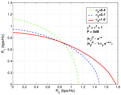
Figure 2: Secrecy capacity regions for Rayleigh fading BCCs

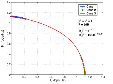
Figure 3: Three cases in power allocation optimization to achieve the boundary of the secrecy capacity region for a Rayleigh fading BCC

For the Rayleigh fading BCC with $\sigma_{1}=1$ and $\sigma_{2}=0.4$, we plot the boundary of the secrecy capacity region in Fig. 3. The three cases (see Theorem 2) to derive the boundary achieving power allocations are also indicated with the corresponding boundary points. It can be seen that the boundary points with large $R_{1}$ are achieved by the power allocations derived from Case 1, and are indicated by the line with circle on the graph. The boundary points with large $R_{0}$ are achieved by the optimal power allocations derived from Case 2, and are indicated by the line with square. Between the boundary points achieved by Case 1 and Case 2, the boundary points are achieved by the power allocations derived from Case 3, and are indicated by the plain solid line.

An intuitive reason why the three cases associate with the boundary points is given as follows. To achieve large secrecy rate $R_{1}$, most channel states in the set $A$ where receiver 1 has a stronger channel than receiver 2 are used to transmit the confidential message. The common message is hence transmitted mostly over the channel states in the set $A^{c}$, over which the common rate is limited by the channel from the source node to receiver 1. Thus, power allocation needs to optimize the rate of this channel, and hence the optimal power allocation follows from Case 1. To achieve large $R_{0}$, the common message is forwarded over the channel states both in $A$ and $A^{c}$. Since in average the source node has a much worse channel to receiver 2 than to receiver 1, the channel from the source node to receiver 2 limits the common rate. Power allocation now needs to optimize the rate to receiver 2, and hence follows from Case 2. Between these two cases, power allocation needs to balance the rates to receivers 1 and 2 and hence follows from Case 3.

IV Conclusions

We have established the secrecy capacity region for the parallel Gaussian BCC, and have characterized the optimal power allocations that achieve the boundary of this region. An interesting result we have established is the secrecy capacity region of the Gaussian case of the Csisz$\acute{\text{a}}$r and K$\ddot{\text{o}}$rner BCC model.

We have further applied our results to obtain the ergodic secrecy capacity region for the fading BCC. Our results generalize the secrecy capacity of the fading wire-tap channel that has been recently obtained in [12], [13] and [14] (full CSI case). We have also studied the outage performance of the fading BCC, the results of which are not presented in this paper due to space limitations; details can be found in [16].

References

- [1] A. D. Wyner, “The wire-tap channel,” Bell Syst. Tech. J., vol. 54, no. 8, pp. 1355–1387, Oct. 1975.
- [2] S. K. Leung-Yan-Cheong and M. E. Hellman, “The Gaussian wire-tap channel,” IEEE Trans. Inform. Theory, vol. 24, no. 4, pp. 451–456, July 1978.
- [3] P. Parada and R. Blahut, “Secrecy capacity of SIMO and slow fading channels,” in Proc. IEEE Int. Symp. Information Theory (ISIT), Adelaide, Australia, Sept. 2005, pp. 2152–2155.
- [4] J. Barros and M. R. D. Rodrigues, “Secrecy capacity of wireless channels,” in Proc. IEEE Int. Symp. Information Theory (ISIT), Seattle, WA, USA, July 2006.
- [5] I. Csiszr and J. Krner, “Broadcast channels with confidential messages,” IEEE Trans. Inform. Theory, vol. 24, no. 3, pp. 339–348, May 1978.
- [6] R. Liu, I. Maric, P. Spasojevic, and R. Yates, “Discrete memoryless interference and broadcast channels with confidential messages,” in Proc. Annu. Allerton Conf. Communication, Control and Computing, Monticello, IL, USA, Sept. 2006.
- [7] D. Hughes-Hartogs, “The capacity of the degraded spectral Gaussian broadcast channel,” Ph.D. dissertation, Stanford University, 1975.
- [8] D. N. Tse, “Optimal power allocation over parallel Gaussian broadcast channels,” in Proc. IEEE Int. Symp. Information Theory (ISIT), Ulm, Germany, June 1997, p. 27.
- [9] L. Li and A. J. Goldsmith, “Capacity and optimal resource allocation for fading broadcast channels-Part I: ergodic capacity,” IEEE Trans. Inform. Theory, vol. 47, no. 3, pp. 1083–1102, Mar. 2001.
- [10] ——, “Capacity and optimal resource allocation for fading broadcast channels-Part II: outage capacity,” IEEE Trans. Inform. Theory, vol. 47, no. 3, pp. 1103–1127, Mar. 2001.
- [11] N. Jindal and A. Goldsmith, “Optimal power allocation for parallel Gaussian broadcast channels with independent and common information,” in Proc. IEEE Int. Symp. Information Theory (ISIT), Chicago, Illinois, USA, June-July 2004.
- [12] Y. Liang and H. V. Poor, “Secure communication over fading channels,” in Proc. 44th Annu. Allerton Conf. Communication, Control and Computing, Monticello, IL, USA, Sept. 2006.
- [13] Z. Li, R. Yates, and W. Trappe, “Secrecy capacity of independent parallel channels,” in Proc. 44th Annu. Allerton Conf. Communication, Control and Computing, Monticello, IL, USA, Sept. 2006.
- [14] P. Gopala, L. Lai, and H. El Gamal, “On the secrecy capacity of fading channels,” submitted to IEEE Trans. Inform. Theory, Oct. 2006.
- [15] H. Yamamoto, “A coding theorem for secret sharing communication systems with two Gaussian wiretap channels,” IEEE Trans. Inform. Theory, vol. 37, no. 3, pp. 634–638, May 1991.
- [16] Y. Liang, H. V. Poor, and S. Shamai (Shitz), “Secure communication over fading channels,” submitted to IEEE Trans. Inform. Theory, Nov. 2006; available at http://arxiv.org/PScache/cs/pdf/0701/0701024.pdf.