Structure and Evolution of Giant Cells in Global Models of Solar Convection

Abstract

The global scales of solar convection are studied through three-dimensional simulations of compressible convection carried out in spherical shells of rotating fluid which extend from the base of the convection zone to within 15 Mm of the photosphere. Such modelling at the highest spatial resolution to date allows study of distinctly turbulent convection, revealing that coherent downflow structures associated with giant cells continue to play a significant role in maintaining the strong differential rotation that is achieved. These giant cells at lower latitudes exhibit prograde propagation relative to the mean zonal flow, or differential rotation, that they establish, and retrograde propagation of more isotropic structures with vortical character at mid and high latitudes. The interstices of the downflow networks often possess strong and compact cyclonic flows. The evolving giant-cell downflow systems can be partly masked by the intense smaller scales of convection driven closer to the surface, yet they are likely to be detectable with the helioseismic probing that is now becoming available. Indeed, the meandering streams and varying cellular subsurface flows revealed by helioseismology must be sampling contributions from the giant cells, yet it is difficult to separate out these signals from those attributed to the faster horizontal flows of supergranulation. To aid in such detection, we use our simulations to describe how the properties of giant cells may be expected to vary with depth, how their patterns evolve in time, and analyze the statistical features of correlations within these complex flow fields.

1. Introduction

The highly turbulent solar convection zone serves as a laboratory to guide our understanding of the complex transport mechanisms for heat and angular momentum that exist within rotating stars. One challenge is to explain the strong differential rotation that is observed in the Sun, and is likely to be also realized in many other stars. Another concerns the Sun’s evolving magnetism with its cyclic behavior, which must arise from dynamo processes operating deep within its interior. Both encourage the development of theoretical models capable of studying the coupling of convection, magnetism, rotation and shear under nonlinear conditions. We have approached these challenges by turning to numerical simulations of turbulent convection enabled by rapid advances in supercomputing, and to helioseismology that provides an observational perspective of the interior dynamics. We report here on our three-dimensional simulations of compressible convection carried out in rotating spherical shells that capture many of the attributes of the solar convection zone. The evolving solutions discussed here are obtained from the most turbulent high-resolution simulations conducted so far on massively parallel machines. Such modelling permits us to assess, with hopefully increasing fidelity, the likely properties of large-scale convection expected to be present over a wide range of depths within the solar interior. In this paper we will describe and analyze the features of such giant-cell convection, and in a subsequent paper assess how signatures of these flows may be searched for using helioseismic probing.

Helioseismology has shown that a broad variety of solar subsurface flows are detectable in the upper reaches of the solar convection zone. These range from evolving meridional circulations, to propagating bands of zonal flow speedup, to varying cellular flows and meandering streams involving a wide range of horizontal scales (Haber et al., 2002, 2004; Zhao & Kosovichev, 2004; Hindman et al., 2004, 2006; Komm et al., 2004, 2005, 2007; González-Hernandez et al., 2006). Such detailed probing of flows, loosely designated as solar subsurface weather (SSW), has become feasible through recent advances in local-domain helioseismology that complement earlier studies of large-scale dynamics, such as inferences of the differential rotation, using global oscillation modes (e.g. Thompson et al., 2003). In local helioseismology, the acoustic oscillations of the interior being sampled by high-resolution Doppler imaging of the solar surface can be analyzed over many localized domains to deduce the underlying flow fields, variously using ring-diagram, time-distance and holographic techniques (e.g. Gizon & Birch, 2005).

The horizontal resolution in such helioseismic flow probing, using for instance inversions of acoustic wave frequency splittings measured by ring analyses, can be of order $1^{\circ}$ in sampling the upper few Mm just below the surface, and increases with depth, becoming of order $4^{\circ}$ at a depth of about 10 Mm. This suggests that one can search for explicit signatures of the largest scales of solar convection, or giant cells, which are a prominent feature in deep-shell simulations of convection zone dynamics (e.g. Miesch et al., 2000; Brun & Toomre, 2002; Brun et al., 2004), but which are not readily evident as patterns in surface Doppler measurements. The presence of the fast and evolving flows of granulation and supergranulation, with combined rms horizontal flow amplitudes of order 500 m s^-1, may serve to mask the anticipated weaker flows of giant cells. The helioseismic sampling at depths of a few Mm or greater, where the granular signal is likely to be sharply diminished and the supergranular one beginning to decrease, may thus afford unique ways to search for the largest scales of solar convection.

We will here use our highest resolution, and thus most turbulent, spherical shell simulations of solar convection to assess the possible character of the giant cells. We recognize that our solutions are at best a highly simplified view of the dynamics proceeding deep within the sun. The real sun may well possess more complex flows, or possibly even greater order in the form of coherent structures, since turbulence constrained by rotation, sphericity and stratification can exhibit surprising behavior (e.g. Toomre, 2002). Further, our simulations here cannot yet deal explicitly with either the near-surface shear layer nor with the tachocline, concentrating instead on the bulk of the convection zone. However, we believe it prudent to use these models to provide some guidance and perspective for what may be sought with local helioseismic probing as the search for solar giant cells continues. The flows of SSW likely contain some signals from giant-cell convection over a range of depths (e.g. Haber et al., 2002; Hindman et al., 2004), as do power spectra of surface Doppler measurements (e.g. Hathaway et al., 2000). We will in §3 discuss the nature of the convective structures realized in our simulations, in §4 analyze the differential rotation and meridional circulations that are established, in §5 show how the coherent downflow structures of the giant cells can be identified and tracked with time, and in §6-7 consider the flow statistics and spectra of our global-scale convection. In a subsequent paper we shall concentrate on discussions of what may be required to try to resolve and possibly track the evolution of giant cells by helioseismic means.

2. Model Description

2.1. The ASH Code

The anelastic spherical harmonic (ASH) code solves the three-dimensional equations of fluid motion in a rotating spherical shell under the anelastic approximation. Details on the numerical method can be found in Clune et al. (1999) and Brun et al. (2004) and a discussion of the anelastic approximation in Gough (1969), Glatzmaier & Gilman (1981a), Lantz & Fan (1999), and Miesch (2005). What follows is a brief summary of the physical model and computational algorithm.

The anelastic equations expressing conservation of mass, momentum, and energy are given by

$$\mbox{\boldmath$\nabla\mbox{\boldmath$\cdot$}$}(\overline{\rho}{\bf v})=0,$$ (1)

$$\overline{\rho}\frac{\partial{\bf v}}{\partial t}+\overline{\rho}({\bf v}\cdot\mbox{\boldmath$\nabla$}){\bf v}=-\mbox{\boldmath$\nabla$}P-\rho g\mbox{\boldmath$\hat{r}$}-2\overline{\rho}(\mbox{\boldmath$\Omega_{*}$}\mbox{\boldmath$\times$}{\bf v})\\ -\mbox{\boldmath$\nabla\mbox{\boldmath$\cdot$}$}\mbox{\boldmath${\cal D}$}-\mbox{\boldmath$\hat{r}$}\left[\frac{d\overline{P}}{dr}+\overline{\rho}g\right]$$ (2)

$$\overline{\rho}\overline{T}\left(\frac{\partial S}{\partial t}+{\bf v}\cdot\mbox{\boldmath$\nabla$}S\right)=-\overline{\rho}\overline{T}v_{r}\frac{d\overline{S}}{dr}\\ +\mbox{\boldmath$\nabla\mbox{\boldmath$\cdot$}$}\left[\kappa_{r}\overline{\rho}C_{P}\mbox{\boldmath$\nabla$}\left(T+\overline{T}\right)+\kappa\overline{\rho}\overline{T}\mbox{\boldmath$\nabla$}\left(S+\overline{S}\right)\right]+\Phi~{}~{}~{}.$$ (3)

These equations are expressed in a spherical polar coordinate system rotating with an angular velocity of $\Omega_{*}$, with radius $r$, colatitude $\theta$, and longitude $\phi$. The corresponding unit vectors are $\hat{r}$, $\hat{\theta}$, $\hat{\phi}$ and the velocity components are given by ${\bf v}=v_{r}\mbox{\boldmath$\hat{r}$}+v_{\theta}\mbox{\boldmath$\hat{\theta}$}+v_{\phi}\mbox{\boldmath$\hat{\phi}$}$. The density $\rho$, pressure $P$, temperature $T$, and specific entropy $S$ are perturbations relative to a spherically-symmetric reference state represented by $\overline{\rho}$, $\overline{P}$, $\overline{T}$, and $\overline{S}$. This reference state evolves in time, being periodically updated by the spherically-symmetric component of the perturbations. Since convective motions contribute to the force balance, the final term on the right-hand-side of equation (2) is generally nonzero. The gravitational acceleration $g$ and the radiative diffusivity $\kappa_{r}$ are independent of time but vary with radius.

The components of the viscous stress tensor ${\cal D}$ are given by

$${\cal D}_{ij}=-2\overline{\rho}\nu\left[e_{ij}-\frac{1}{3}\left(\mbox{\boldmath$\nabla\mbox{\boldmath$\cdot$}$}{\bf v}\right)\delta_{ij}\right]$$ (4)

and the viscous heating term is given by

$$\Phi=2\overline{\rho}\nu\left[e_{ij}e_{ij}-\frac{1}{3}\left(\mbox{\boldmath$\nabla\mbox{\boldmath$\cdot$}$}{\bf v}\right)^{2}\right]~{}~{}~{}.$$ (5)

In these expressions $e_{ij}$ is the strain rate tensor and $\delta_{ij}$ is the Kronecker delta. Summation over $i$ and $j$ is implied in equation (5). The kinematic viscosity $\nu$ and the thermal diffusivity $\kappa$ represent transport by unresolved, subgrid-scale (SGS) motions. In this paper they are assumed to be constant in space and time in order to minimize diffusion in the upper convection zone, which is of most interest from the perspective oof helioseismology.

The vertical vorticity $\zeta$ and the horizontal divergence $\Delta$ are defined as

$$\zeta=\left(\mbox{\boldmath$\nabla\times$}{\bf v}\right)\mbox{\boldmath$\cdot$}\mbox{\boldmath$\hat{r}$}$$ (6)

and

$$\Delta=\mbox{\boldmath$\nabla\mbox{\boldmath$\cdot$}$}\left(v_{\theta}\mbox{\boldmath$\hat{\theta}$}+v_{\phi}\mbox{\boldmath$\hat{\phi}$}\right)~{}~{}~{}.$$ (7)

Equations (1)–(5) are solved using a pseudospectral method with spherical harmonic and Chebyshev basis functions. A second-order Adams-Bashforth/Crank-Nicolson technique is used to advance the solution in time and the mass flux is expressed in terms of poloidal and toroidal streamfunctions such that equation (1) is satisfied at all times. The ASH code is written in FORTRAN 90 using the MPI (Message Passing Interface) library, and is optimized for efficient performance on scalably parallel computing platforms.

2.2. Simulation Summary

In previous papers based on ASH simulations we have investigated parameter sensitivities, convective structure and transport, the maintenance of differential rotation and meridional circulation, and hydromagnetic dynamo processes (Miesch et al., 2000; Elliott et al., 2000; Brun & Toomre, 2002; Brun et al., 2004; Miesch et al., 2006; Browning et al., 2006). In this paper we focus on a single, representative high-resolution simulation and discuss aspects of the flow field which can potentially be probed by helioseismology.

The simulation domain extends from the base of the convection zone $r_{1}=0.71R$ to $r_{2}=0.98R$, where $R$ is the solar radius. Thus, the upper boundary is about 14 Mm below the photosphere. Beyond $r=0.98R$ the anelastic approximation begins to break down and ionization effects become important. The small-scale convection which ensues (granulation) cannot currently be resolved by any global model. We assume that the boundaries are impermeable and free of tangential stresses.

At the lower boundary we impose a latitudinal entropy gradient as discussed by Miesch et al. (2006). This is intended to model the thermal coupling between the convection zone and the radiative interior through the tachocline. If the tachocline is in thermal wind balance as suggested by many theoretical and numerical models, then the rotational shear inferred from helioseismology implies a relative latitudinal entropy variation $S/C_{P}\sim 4\times 10^{-6}$ where $C_{P}$ is the specific heat at constant pressure. This corresponds to a temperature variation of about 10K, monotonically increasing from equator to pole. We implement this by setting

$$\frac{S(\theta)}{C_{P}}=a_{2}Y_{2}^{0}+a_{4}Y_{4}^{0}$$ (8)

at $r=r_{1}$, where $Y_{\ell}^{m}$ is the spherical harmonic of degree $\ell$ and order $m$. Here we take $a_{2}=2.7\times 10^{-6}$ and $a_{4}=-6.04\times 10^{-7}$. For further details see Miesch et al. (2006). For the upper thermal boundary condition we impose a constant heat flux by fixing the radial entropy gradient.

Solar values are used for the luminosity $L_{*}=3.846\times 10^{33}$ erg s^-1 and the rotation rate $\Omega_{*}=2.6\times 10^{-6}$ rad s^-1. The reference state, the gravitational acceleration $g$, and the radiative diffusion $\kappa_{r}$ are based on a 1–D solar structure model as described by Christensen-Dalsgaard et al. (1996). The density contrast across the convection zone $\overline{\rho}(r_{1})/\overline{\rho}(r_{2})=132$ which is more than three times higher than any previous simulation of global-scale solar convection. This large density contrast plays an important role in many aspects of the flow field, including the scale of the downflow network near the surface and the asymmetry between upflows and downflows. Previous simulations did not have sufficient spatial resolution to capture such dynamics.

Figure 1.— Snapshots of the radial velocity $v_{r}$ at ($a$) $r=0.98R$ and ($b$) $r=0.95R$. Bright and dark tones indicate upflow and downflow respectively as indicated by the color bar. The horizontal surfaces are displayed in a Molleweide projection which includes all 360^∘ of longitude and in which lines of constant latitude are horizontal. Dashed lines indicate latitudes of $0^{\circ}$, $\pm 30^{\circ}$, and $\pm 60^{\circ}$ and longitudes of $0^{\circ}$ and $\pm 90^{\circ}$.

The spatial resolution $N_{r}=257$, $N_{\theta}=1024$, and $N_{\phi}=2048$ is higher than in any previously published simulation of global-scale solar convection. In our triangular truncation of the spherical harmonic series representation, this corresponds to a maximum degree of $\ell_{max}=682$. High resolution has enabled us to achieve turbulent parameter regimes that were inaccessible in previous simulations. We set $\nu=1.2\times 10^{12}$ cm² s^-1 and $\kappa=4.8\times 10^{12}$ cm² s^-1 throughout the computational domain, yielding a Prandtl number $P_{r}=\nu/\kappa=0.25$. The velocity amplitude varies from about 250 m s^-1 near the top of the shell to about 50 m s^-1 near the bottom (Fig. 15$a$). If we take the length scale to be the depth of the convection zone, $D=$ 187 Mm, then the Reynolds number near the top of the shell is $R_{e}=UD/\nu\sim 400$. The Rossby number, $R_{o}=U/(2\Omega_{*}D)$, varies from 0.26 near the top of the convection zone to 0.05 near the bottom, indicating a strong rotational influence on the convective motions. However, the Rossby number based on the standard deviation of the vertical vorticity near the top of the convection zone, $\sigma_{\zeta}=2\times 10^{-5}$, is much larger; $R_{o}=\sigma_{\zeta}/2\Omega_{*}\sim 4$. Thus, the small-scale, intermittent downflows where most of the vorticity is concentrated are less influenced by rotation.

Figure 2.— Snapshot of convective patterns near the surface. The four columns illustrate ($a$) radial velocity $v_{r}$, ($b$) radial vorticity $\zeta$, ($c$) horizontal divergence $\Delta$, and ($d$) temperature $T$. The orthographic projections in the top row correspond to $r=0.98R$ and the north pole is tilted 35^∘ toward the observer. The three rows below show a $45^{\circ}\times 45^{\circ}$ patch in latitude (10^∘–55^∘) and longitude at $r=0.98R$, $0.95R$, and $0.92R$. Color tables for each column are indicated below the $0.98R$ patch but scaling varies with depth. The scales indicated on the color bar correspond to the $0.98R$ projections (upper two rows) while the scales used for the deeper layers are indicated below each image.

3. Overview of Convective Structure

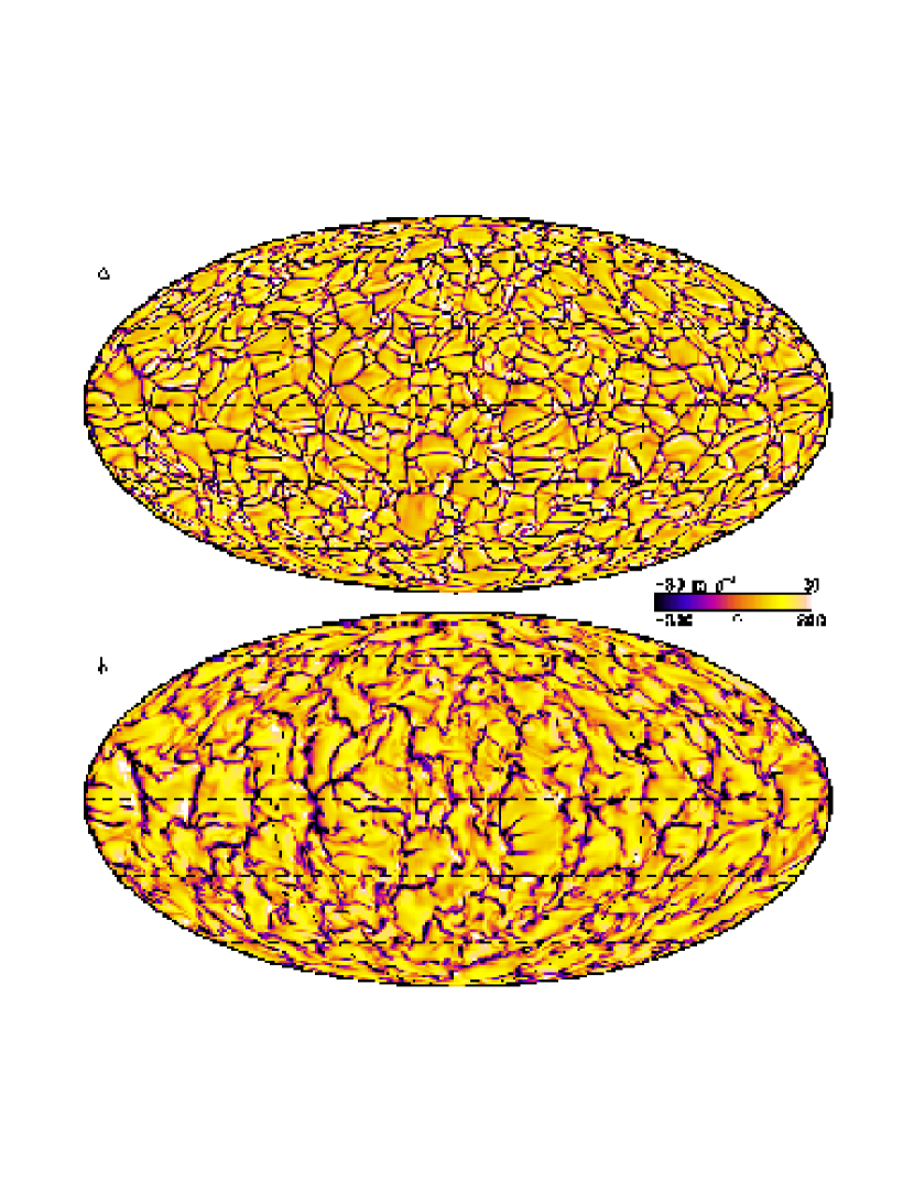
Figure 1 is a representative example of the convective patterns achieved in the upper portion of the convection zone. Near the top of our computational domain at $r=0.98R$, the structure of the convection resembles solar granulation but on a much larger scale; an interconnected network of strong downflow lanes surrounds a disconnected distribution of broader, weaker upflows. The dramatic asymmetry between upflows and downflows can be attributed primarily to the density stratification, and is a characteristic feature of compressible convection. As fluid flows upward, it diverges horizontally due to mass conservation. Upflows thus have a larger filling factor than downflows and are correspondingly less intense.

By $r=0.95R$ the downflow network begins to fragment, but isolated, intermittent downflow lanes and plumes remain. At low latitudes, many of the strongest downflow lanes have a north-south orientation. These NS (north-south) downflow lanes represent the dominant coherent structures in the flow at low latitudes and we will discuss them repeatedly throughout this paper. They can be identified within the intricate downflow network near the surface but they are more prominent deeper in the convection zone.

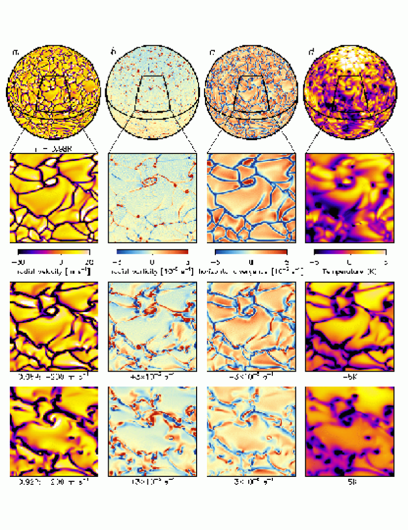
The downflow network near the surface evolves rapidly, with a correlation time of several days (§5). Convection cells interact with one another and are advected, distorted, and fragmented by the rotational shear. At mid and high latitudes, downflows posses intense radial vorticity as demonstrated in Figure 2$a$, $b$. The sense of this vorticity is generally cyclonic, implying a counter-clockwise circulation in the northern hemisphere and a clockwise circulation in the southern hemisphere (more generallly, the vorticity vector is referred to as cyclonic if it has a component parallel to the rotation vector and anticyclonic if antiparallel). The vorticity peaks at the intersticies of the downflow network in localized vortex tubes which we refer to as high-latitude cyclones. Vortex sheets also occur in more extended downflow lanes.

The cyclonic vorticity in downflow lanes arises from Coriolis forces acting on horizontally converging flows. Near the top of the convection zone there is a strong correlation between vertical velocity and horizontal divergence as demonstrated in Figure 2$a$, $c$. This is as expected from mass conservation; as upflows approach the impenetrable boundary they diverge due to the density stratification and eventually overturn, with regions of horizontal convergence feeding mass into the downflow lanes. Fluid parcels tend to conserve their angular momentum, giving rise to weak anticyclonic vorticity in diverging upflows and stronger cyclonic vorticity in narrower downflow lanes. Thus, the kinetic helicity of the flow, defined as the scalar product of the vorticity and the velocity, is negative throughout most of the convection zone, changing sign only near the base where downflows diverge horizontally upon encountering the lower boundary (Miesch et al., 2000; Brun et al., 2004).

The thermal nature of the convection is evident in Figure 2$a$, $d$; upflows are generally warm and downflows cool. The more diffuse appearence of the temperture structure relative to the vertical velocity structure may be attributed to the low Prandtl number $P_{r}=0.25$. The most extreme temperature variations are cool spots associated with the high-latitude cyclones. Global-scale temperature variations are also evident in Figure 2$d$, in particular the poles are on average 6-8K warmer than the equator. This is associated with thermal wind balance of the differential rotation as discussed in §4.

Figure 3.— Radial energy flux as a function of radius, integrated over horizontal surfaces and averaged over time (62 days). Components include $F_{e}$ (solid line), $F_{r}$ (dashed), $F_{k}$ (dot-dash), and $F_{u}$ (dot-dot-dash), all normalized by the solar flux $F_{*}=L_{*}/(4\pi r^{2})$. The sum of these four components is shown as a thick solid line. Vertical dotted lines indicate the radial levels illustrated in Fig. 2.

The correlation between temperature and vertical velocity gives rise to an outward enthalpy flux as illustrated in Figure 3. The convective enthalpy flux $F_{e}$ dominates the other flux components throughout most of the convection zone and peaks at $r=0.92R$ where its integrated luminosity exceeds the solar luminosity $L_{*}$ by as much as 70%. This is a consequence of the pronounced asymmetry between upflows and downflows. The greater intensity of the latter gives rise to a large downward kinetic energy flux $F_{k}$ ($\propto v^{2}v_{r}$) which must be compensated for by the upward enthalpy flux (Fig. 3). This has important consequences for 1-D solar structure models based on mixing length theory which generally neglect $F_{k}$ and thus assume that the integrated convective enthalpy flux in the convection zone is equal to $L_{*}$.

Near the boundaries both $F_{e}$ and $F_{k}$ drop to zero due to the impenetrable boundary conditions. Flux is carried through the boundaries by radiative diffusion $F_{r}$ and subgrid-scale (SGS) thermal diffusion $F_{u}$, the latter of which is proportional to the radial entropy gradient $\partial\overline{S}/\partial r$. Viscous heat transport is negligible and is therefore omitted from Figure 3. Complete expressions for $F_{e}$, $F_{k}$, $F_{r}$, and $F_{u}$ are given in Brun et al. (2004).

Figure 4.— Radial velocity $v_{r}$ at four horizontal levels ($a$) $0.98R$, ($b$) $0.92R$, ($c$) $0.85R$, and ($d$) $0.71R$. The color table is as in Fig. 1, with the range indicated in each frame. Each image is an orthographic projection with the north pole tilted $35^{\circ}$ toward the line of sight. The dotted line indicates the solar radius $r=R$.

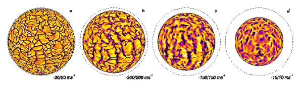
The variation of convective structure with depth throughout the entire convection zone is illustrated in Figure 4. As noted with regard to Figure 1, the downflow network near the surface loses its connectivity deeper down but isolated downflow lanes and plumes persist. The strongest lanes and plumes remain coherent across the entire convection zone, spanning approximately 190 Mm and 4.9 density scale heights. The low-latitude NS (north-south) downflow lanes identified in Figure 1 are most prominent in the mid convection zone; near the surface they merge with the more homogeneous downflow network and near the base of the convection zone they fragment into more isolated plumes. By contrast, the high-latitude cyclones identified in Figure 2 are largely confined to the upper convection zone.

Figure 5.— The enstrophy ($\omega^{2}$, where $\mbox{\boldmath$\omega$}=\mbox{\boldmath$\nabla\times$}{\bf v}$) shown for a 45^∘ $\times$ 45^∘ patch in latitude ($10^{\circ}$-55^∘) and longitude at ($a$) $r=0.98R$ and ($b$) $r=0.85R$. The color table is as in Fig. 1 but here scaled logarithmically. Ranges shown are ($a$) $10^{-12}$ to $10^{-7}$ s^-2 and ($b$) $10^{-13}$ to $10^{-8}$ s^-2.

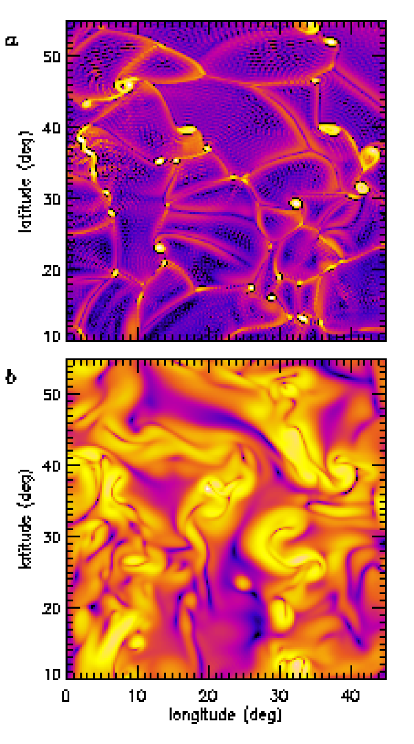
As in many turbulent flows, the enstrophy (the square of the vorticity vector) provides a useful means to probe coherent structures within the flow. Figure 5 illustrates the enstrophy in a square patch in the upper and mid convection zone. Near the surface, the high-latitude cyclones dominate the enstrophy, and the vorticity is predominantly radial (Fig. 5$a$). The high spatial intermittency of these vortex structures produces some Gibbs ringing in the enstrophy field but this becomes neglible deeper in the convection zone. The enstrophy in the mid convection zone is dominated by vortex sheets associated with turbulent entrainment which line the periphery of downflow lanes and plumes (Fig. 5$b$). Such horizontal entrainment vorticies also line the downflow network at $r=0.98R$ but they are generally weaker than the vertically-aligned cyclones (Fig. 5$a$).

4. Differential Rotation and Meridional Circulation

A primary motivation behind simulations of global-scale convection in the solar envelope is to provide further insight into the maintenance of differential rotation and meridional circulation. These axisymmetric flow components play an essential role in all solar dynamo models and have been probed extensively by helioseismology and surface measurements. Although the focus of this paper is on the structure and evolution of global-scale convective patterns, it is important to briefly describe the nature of the mean flows produced and maintained in our simulation.

Figure 6.— Differential rotation, meridional circulation, and mean temperature perturbation averaged over longitude and time (58 days). The angular velocity shown ($a$) as a 2-D image and ($b$) as a function of radius for selected latitudes as indicated. Contour levels in ($a$) are every 10 nHz and the rotation rate of the coordinate system (414 nHz) is indicated on the color bar (black line). Contours of the streamfunction $\Psi$ in ($c$) represent streamlines of the mass flux with red (black contours) and blue (grey contours) representing clockwise and counter-clockwise circulation respectively. The color table saturates at $\Psi=\pm 1.08\times 10^{22}$ g s^-1. Characteristic amplitudes for $\left<v_{\theta}\right>$ are 20 m $s^{-1}$ (poleward) at $r=0.95R$ and 5 m s^-1 (equatorward) at $r=0.75R$. Contour levels for the temperature perturbation ($d$) are every 1K.

The differential rotation may be expressed in terms of the mean angular velocity $\Omega=\Omega_{*}+\left<v_{\phi}\right>/(r\sin\theta)$ and the meridional circulation may be described by a mass flux streamfunction $\Psi$ defined such that

$$\overline{\rho}\left<v_{r}\right>=\frac{1}{r^{2}\sin\theta}\frac{\partial\Psi}{\partial\theta}\mbox{, and }\overline{\rho}\left<v_{\theta}\right>=-\frac{1}{r\sin\theta}\frac{\partial\Psi}{\partial r}~{}~{}~{}.$$ (9)

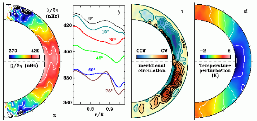
Angular brackets $<>$ denote an average over longitude. Equation (9) applies when the divergence of the mass flux vanishes as required by the anelastic approximation. Time averages of $\Omega$ and $\Psi$ are shown in Figure 6.

The angular velocity profile is similar to the solar internal rotation profile inferred from helioseismic measurements (Thompson et al., 2003), although the variation is smaller and there is somewhat more radial shear within the convection zone. The mean angular velocity decreases by about 50 nHz (11%) from the equator to latitudes of 60 degrees, compared to about 90 nHz in the Sun. This difference may arise from viscous diffusion which, although lower than in previous models is still higher than in the Sun, or from thermal and mechanical coupling to the tachocline which is only crudely incorporated into this model through our lower boundary conditions (Miesch et al., 2006). For example, perhaps the tachocline is thinner, and the associated entropy variation correspondingly larger, than what we have imposed (§2). More laminar models have more viscous diffusion but they also have larger Reynolds stresses so many are able to maintain a stronger differential rotation, some with conical angular velocity contours as in the Sun (Elliott et al., 2000; Brun & Toomre, 2002; Miesch et al., 2006). A more complete understanding of how the highly turbulent solar convection zone maintains such a large angular velocity contrast requires further study.

At latitudes above 30^∘ the angular velocity increases by about 4-8 nHz (1-2%) just below the outer boundary ($r$ = 0.95$R$-0.98$R$). This is reminiscent of the subsurface shear layer inferred from helioseismology but its sense is opposite; in the Sun the angular velocity gradient is negative from $r$ = 0.95$R$ to the photosphere (Thompson et al., 2003). This discrepancy likely arises from our impenetrable, stress-free, constant-flux boundary conditions at the outer surface of our computational domain, $r=0.98R$. In the Sun, giant-cell convection must couple in some way to the supergranulation and granulation which dominates in the near-surface layers. Such motions cannot presently be resolved in a global three-dimensional simulation and involve physical processes such as radiative transfer and ionization which lie beyond the scope of our model.

The meridional circulation is dominated by a single cell in each hemisphere, with poleward flow in the upper convection zone and equatorward flow in the lower convection zone (Fig. 6$c$). At a latitude of 30^∘, the transition between poleward and equatorward flows occurs at $r\sim$ 0.84-0.85 $R$. These cells extend from the equator to latitudes of about 60^∘. The sense (poleward) and amplitude (15-20 m s^-1), of the flow in the upper convection zone is comparable to meridional flow speeds inferred from local helioseismology and surface measurements (Komm et al., 1993; Hathaway, 1996; Braun & Fan, 1998; Haber et al., 2002; Zhao & Kosovichev, 2004; González-Hernandez et al., 2006). The equatorward flow in the lower convection zone peaks at $r\sim 0.75R$ with an amplitude of 5-10 m s^-1.

Near the upper and lower boundaries there are thin counter cells where the latitudinal velocity $\left<v_{\theta}\right>$ reverses. The presence of these cells is likely sensitive to the boundary conditions and must therefore be interpreted with care. Global-scale convection in the Sun couples to the underlying radiative interior via the tacholine and to the overlying photospheric convection (granulation, supergranulation) in complex ways which are not yet well understood. The sense and amplitude of the meridional circulation is coupled to the differential rotation by the requirement that the time-averaged angular momentum transport by advection balance that due to Reynolds stresses. The weak counter cell near the upper boundary (where the flow is equatorward) is thus related to the positive radial angular velocity gradient at high latitudes seen in Figure 6$b$ and may arise from a misrepresentation of the Reynolds stresses at the boundary. Likewise, the counter cell near the lower boundary may be sensitive to the absence of a tachocline and overshoot region. Previous simulations which include convective penetration tend to exhibit equatorward meridional circulations throughout the lower convection zone and overshoot region (Miesch et al., 2000). Further work is needed to clarify the complex dynamics at the top and the bottom of the solar convection zone and what effect it has on mean flow patterns.

Figure 7.— ($a$) Radial and ($b$) latitudinal transport of angular momentum as expressed in equations (10)-(15), averaged over a time interval of 112 days (four rotation periods). Shown are contributions due to Reynolds stresses (RS, solid lines), meridional circulation (MC, dashed lines), and viscous diffusion (VD, dotted lines). Zero is indicated by the dash-dotted line.

Figure 7 illustrates angular momentum transport in our simulation including contributions from Reynolds stresses ($RS$), meridional circulation ($MC$), and viscous diffusion ($VD$). These corresponding fluxes are defined as (Elliott et al., 2000; Brun & Toomre, 2002; Brun et al., 2004; Miesch, 2005)

$${\bf F}^{RS}=\overline{\rho}r\sin\theta\left(\left<v_{r}^{\prime}v_{\phi}^{\prime}\right>\mbox{\boldmath$\hat{r}$}+\left<v_{\theta}^{\prime}v_{\phi}^{\prime}\right>\mbox{\boldmath$\hat{\theta}$}\right)$$ (10)

$${\bf F}^{MC}=\overline{\rho}{\cal L}\left(\left<v_{r}\right>\mbox{\boldmath$\hat{r}$}+\left<v_{\theta}\right>\mbox{\boldmath$\hat{\theta}$}\right)$$ (11)

$${\bf F}^{VD}=-\overline{\rho}\nu r^{2}\sin^{2}\theta\mbox{\boldmath$\nabla$}\Omega~{}~{}~{},$$ (12)

where

$${\cal L}=r\sin\theta\left(\Omega r\sin\theta+\left<v_{\phi}\right>\right)$$ (13)

is the specific angular momentum and primes indicate that the longitudinal mean has been removed, e.g. $v_{r}^{\prime}=v_{r}-\left<v_{r}\right>$.

The total angular momentum flux through perpendicular surfaces is obtained by integrating the various components as follows:

$$I_{r}^{i}(r)=\int_{0}^{\pi}F_{r}^{i}(r,\theta)r^{2}\sin\theta~{}d\theta$$ (14)

$$I_{\theta}^{i}(\theta)=\int_{r_{1}}^{r_{2}}F_{\theta}^{i}(r,\theta)r\sin\theta~{}dr~{}~{}~{},$$ (15)

where $i$ corresponds to $RS$, $MC$, or $VD$. Figure 7 shows time averages of these integrated fluxes.

The prograde differential rotation at the equator is maintained primarily by equatorward angular momentum transport induced by Reynolds stresses (Fig. 7$b$). This transport is dominated by the NS downflow lanes discussed in §3 which represent the principal coherent structures at low latitudes (persistent over relatively long times and large horizontal and vertical scales). Coriolis-induced tilts in the horizontally converging flows which feed these downflow lanes give rise to Reynolds stresses which transport angular momentum toward the equator (see Miesch, 2005, Fig. 15).

Reynolds stresses also transport angular momentum inward throughout most of the convection zone (Fig. 7$a$). This is a significant departure from previous simulations of global-scale solar convection which have exhibited an outward transport of angular momentum by Reynolds stresses (Brun & Toomre, 2002; Brun et al., 2004). Inward angular momentum transport by convection is a common feature of many mean-field models in which it is typically parameterized by means of the so-called $\Lambda$-effect (e.g. Kitchatinov & Rüdiger, 1993; Canuto et al., 1994; Kitchatinov & Rüdiger, 2005; Rüdiger et al., 2005). However, in some models this inward transport arises from a velocity anisotropy such that the standard deviation of $v_{r}$ exceeds that of $v_{\phi}$ (e.g. Rüdiger et al., 2005). Such is not the case in our simulation where the three velocity components are comparable in amplitude through most of the convection zone (see Fig. 15$a$). The reversal in $F^{RS}$ and $F^{MC}$ near the boundaries is associated with the counter cells in the meridional circulation seen in Figure 6$c$.

Advection of angular momentum by the meridional circulation gives rise to poleward and outward transport, nearly balancing the Reynolds stresses, while the transport due to viscous diffusion is relatively small. This approximate balance between Reynolds stresses and meridional circulation with regard to angular momentum transport is that which is expected to exist in the convection zone of the Sun and in other stars where Lorentz forces and viscous diffusion are negligible (Tassoul, 1978; Zahn, 1992; Elliott et al., 2000; Rempel, 2005; Miesch, 2005). The curves shown in Figure 7 do not sum precisely to zero, indicating that there is some evolution of the rotation profile over timescales which are longer than the 112-day averaging interval.

The delicate balance between ${\bf F}^{RS}$ and ${\bf F}^{MC}$ plays an essential role in determining what meridional circulation patterns are achieved. In previous global simulations, viscous angular momentum transport was significant and this balance was disrupted. Circulation patterns were generally multi-celled in latitude and radius (Miesch et al., 2000; Elliott et al., 2000; Brun & Toomre, 2002; Brun et al., 2004). By contrast, the circulation patterns shown in Figure 6$b$ are dominated by a single cell in each hemisphere.

Not only is the viscosity lower than in most previous simulations, but this is the first global simulation to extend from the base of the convection zone to $r=0.98R$, spanning a factor of more than 130 in density (§2.2). Furthermore, we have incorporated some aspects of the coupling between the tachocline and the convective envelope into our model by applying a weak latitudinal entropy variation at the bottom boundary (§2.2). As discussed by Miesch et al. (2006), this entropy variation is transmitted throughout the domain by the convective heat flux and the resulting baroclinicity promotes conical angular velocity profiles which satisfy thermal wind balance. Such profiles minimize diffusive angular momentum transport in radius.

The temperature variations associated with thermal wind balance are evident in Figure 6$d$. The poles are about 6-8K warmer than the equator on average. The background temperature varies from 2.2$\times 10^{7}$ K at the base of the convection zone to 8.4$\times 10^{4}$ K at the outer boundary so the relative latitudinal variations are small, $3\times 10^{-6}$ to $10^{-4}$.

Figure 8.— Instantaneous snapshots of the meridional circulation streamlines at five times separated by an interval of 28 days. Color tables and contours are as in Figure 6$c$ but the normalization for $\Psi$ is three times larger, $\pm 3\times 10^{22}$ g s^-1. Peak amplitudes for $v_{\theta}$ reach 60 m s^-1 near the top of the convection zone.

The differential rotation profile is steady in time; instantaneous snapshots appear similar to Figure 6$a$ but with more small-scale structure and somewhat more asymmetry about the equator. For illustration, the amplitude of the temporal variations sampled at a latitude of 30^∘ relative to a two-month mean is $\pm 10$ nHz toward the top of the convection zone ($\sim$ 2%), decreasing to $\pm$ 5 nHz toward the base. Angular velocity variations are larger at high latitudes where the moment arm ($r\sin\theta$) approaches zero. The amplitude and nature of these variations is comparable to solar rotational variations inferred from helioseismology (Thompson et al., 2003). However, in addition to more random fluctuations, the solar rotation exhibits periodic torsional oscillations which are not realized in our simulation. These are associated with magnetic activity which lies beyond the scope of our current model (e.g. Covas et al., 2000; Spruit, 2003; Rempel, 2005, 2007).

By contrast, fluctuations in the meridional circulation are large relative to the temporal mean, changing substantially over the course of one rotation period as illustrated in Figure 8. Variations in the axisymmetric latitudinal velocity $\left<v_{\theta}\right>$ at a latitude of $30^{\circ}$ reach $\pm 60$ m s^-1 at the top of the convection zone and $\pm 10$ m s^-1 near the base, as much as 300% of the two-month mean. Instantaneous circulation patterns are in general multi-celled in latitude and radius and asymmetric about the equator. Some asymmetry persists even in two-month averages (Fig. 6$c$). Large relative variations in the meridional circulation are expected because it is weak relative to the other flow components so it is easily altered by fluctuating Reynolds stresses and Coriolis forces. The volume-integrated kinetic energy contained in the meridional circulation is approximately an order of magnitude smaller than in the differential rotation and approximately two orders of magnitude smaller than in the convection.

Determinations of the solar meridional circulation from surface measurements and helioseismic inversions are generally averaged over at least one rotation period (Komm et al., 1993; Hathaway, 1996; Braun & Fan, 1998; Haber et al., 2002, 2004; Zhao & Kosovichev, 2004; González-Hernandez et al., 2006). The time variations are therefore less than in the snapshots illustrated in Figure 8$f$-$j$ but consistent with comparable running time averages in the simulation. However, as with the angular velocity, systematic variations in the solar meridional circulation associated with the magnetic activity cycle are not captured in this non-magnetic simulation.

5. Identification and Evolution of Coherent Structures

In §3 we described recurring convective features including NS downflow lanes found at low latitudes and intermittent, high-latitude cyclones. In this section we discuss these coherent structures in more detail and address the lifetime, propagation, and evolution of convective patterns.

Figure 9.— Temporal evolution of convective patterns near the equator. Each image shows the radial velocity field at $r=0.98R$ for all 360^∘ of longitude and a latitude range of $0^{\circ}$–$25^{\circ}$. The color table is the same as in Fig. 1$a$. Snapshots at different times are stacked vertically, with time increasing upward. The interval between snapshots is two days. To facilitate comparison, the uppermost image illustrates the convection structure one rotation period (27.4 days at this latitude and radius) prior to the $\Delta t=$28-day image immediately below it. The tracking rate is the rotation rate of the coordinate system, 414 nHz, but the white arrow shows a propagation rate of 450 nHz for reference.

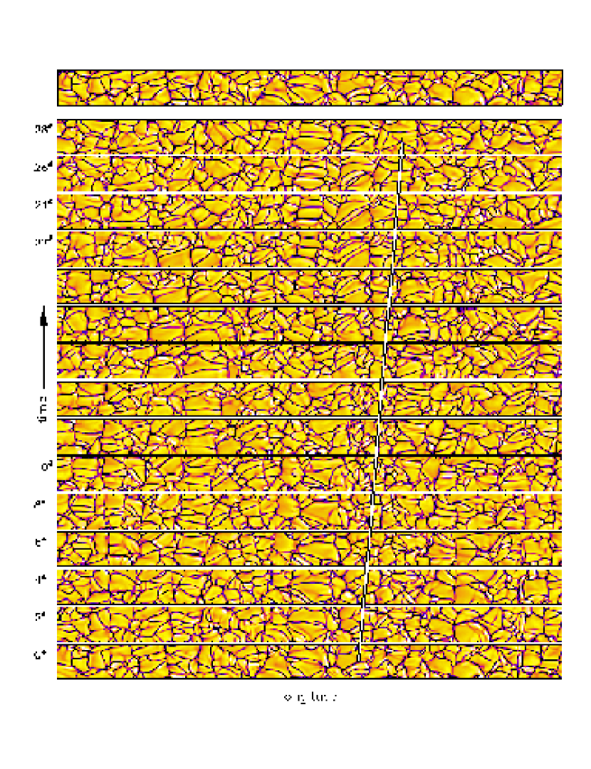
Figure 9 illustrates the evolution of the low-latitude downflow network at $r=0.98R$. Substantial changes are evident even over the two-day time interval between adjacent bands. Individual convection cells typically lose their identity after only a few days and none are clearly recognizable after one rotation period. This has important implications for subsurface weather diagrams inferred from local helioseismology (§1); temporal sampling of a day or less may be necessary to reliably follow the evolution of flow fields associated with giant convection cells.

Embedded within the more rapidly evolving downflow network are features that persist for a month or more. These are the NS downflow lanes discussed in §3, appearing in Figure 9 as dark vertical stripes although it takes some scrutiny to see them amid the complex smaller scales. These propagate in an eastward (prograde) direction relative to the rotating coordinate system as illustrated by the white arrow.

Figure 10.— Time evolution of the zonal velocity derivative $\partial v_{\phi}/\partial\phi$ at $r=0.98R$. The layout and time series corresponds directly with Fig. 9, with bands spanning $0^{\circ}$–$25^{\circ}$ in latitude and time increasing upward. The color table saturates at $\pm 200$ m s^-1; bright tones denote convergence ($\partial v_{\phi}/\partial\phi>0$) and dark tones denote divergence. The white arrow corresponds to an angular velocity of 450 nHz as in Fig. 9.

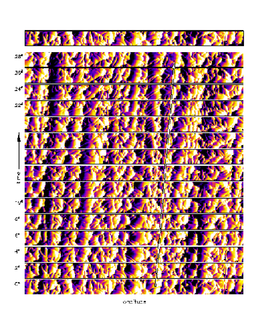
The presence of NS downflow lanes is more readily apparent when the divergence of the zonal velocity $\partial v_{\phi}/\partial\phi$ is plotted as in Figure 10. Whereas the horizontal divergence $\Delta$ corresponds closely to the radial velocity patterns shown in Figure 9, the zonal component alone preferentially selects structures with a north-south orientation. Thus, the NS downflow lanes are more prominent and their prograde propagation and persistence over time scales of at least a month are evident. The propagation rate varies as individual lanes continually catch up to others and subsequently merge.

Figure 11.— Temporal evolution of mid-latitude convection patterns. The radial velocity field is shown at $r=0.98R$ over a square $30^{\circ}\times 30^{\circ}$ patch in latitude and longitude, spanning latitudes of 30^∘–60^∘. The color table is as in Fig. 1$a$. The series shown spans one week, with an interval of one day between successive images. The patch is tracked at an angular velocity of 410 nHz. Labels indicate (A) cyclonic vorticies, (B) dynamical buoyancy, (C) fragmentation and (D) collapse of convection cells, and (E) the persistence of some cells for multiple days.

Using Figure 10 as a reference facilitates the detection of NS downflow lanes within the intricate downflow network of Figure 9. In other words, it is easier to distinguish the NS downflow lanes if one knows where to look. Furthermore, a close comparison of Figures 9 and 10 reveals that the horizontal scale of the convective cells is somewhat smaller in the vicinity of the NS lanes (see, for example, the downflow lane traced by the arrow). This is consistent with the more general characteristic of turbulent compressible convection that downflow lanes tend to be more turbulent and vortical than the broader, weaker upflows (Brummell et al., 1996; Brandenburg et al., 1996; Stein & Nordlund, 1998; Porter & Woodward, 2000; Miesch, 2005, see also Fig. 5). Advection of smaller-scale convection cells and vortices into extended NS downflow lanes is apparent in animations of the radial velocity field.

The longitudinal position of lanes of zonal velocity convergence in the surface layers corresponds closely to the position of NS downflow lanes in the mid convection zone where they are more prominent in the radial velocity field (Fig. 4). Thus, searching for lanes of zonal convergence in solar subsurface weather (SSW) maps inferred from local helioseismology might be a promising way to detect convective structures which extend deep into the convection zone. However, care must be taken when interpreting such results. Even if $v_{\phi}$ were isotropic in latitude and longitude, the one-dimensional derivative $\partial v_{\phi}/\partial\phi$ would still exhibit a preferred north-south orientation. Thus, anisotropy in $\partial v_{\phi}/\partial\phi$ should not be used naively as a criterion for establishing the existence of NS downflow lanes, but it may be used to track the propagation and evolution of such coherent structures if they are indeed present.

The NS downflow lanes are confined to latitudes less than about 30^∘. At higher latitudes the downflow network is more isotropic in latitude and longitude and possesses intense cyclonic vorticity (§3). An illustrative example of the evolution of mid-latitude convective patterns is shown in Figure 11.

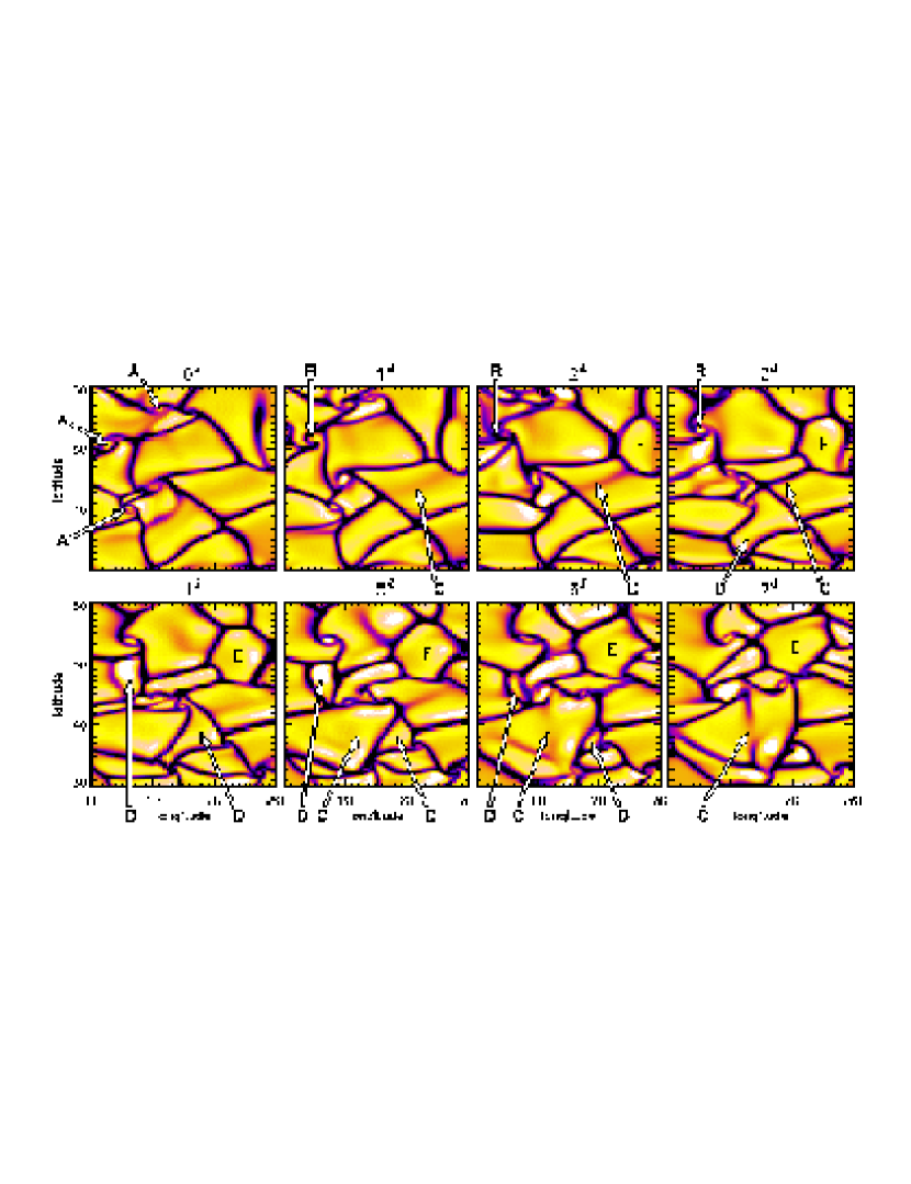
As demonstrated in Figures 2 and 5, intense, vertically-oriented, cyclonic vortices are prevalent throughout the downflow network in the upper convection zone. Centrifugal forces can evacuate the cores of the most intense vorticies, leading to a reversal in the buoyancy driving which siphons fluid up from below and creates a new upflow within the intersticies of the downflow network. This phenomenon has been referred to as dynamical buoyancy and is a characteristic feature of rotating, compressible convection (Brandenburg et al., 1996; Brummell et al., 1996; Miesch et al., 2000). The result is a helical vortex tube with upflow at its center and downflow around its periphery. In the vertical velocity (or the horizontal divergence) field these structures appear as small convection cells, with a horizontal extent comparable to that of supergranulation, about 10-30 Mm. Several examples of these are indicated in Figure 11 (A).

The formation of one of these helical convection cells via dynamical buoyancy is also indicated in Figure 11 (B). At a (relative) time of $1^{d}$, a counter-clockwise swirl can be seen near one of the interstices of the downflow network, reflecting the presence of a vertically-oriented vortex tube. Such cyclonic swirl is evident throughout the downflow network in animations of the flow field. One day later, a strong downflow plume develops and Coriolis forces continue to amplify the cyclonic vorticity. By the next day, centrifugal forces have evacuated the vortex core and reversed the axial flow. After formation, such upflows may spread horizontally due to the density stratification or they may dissipate through interactions with surrounding flows.

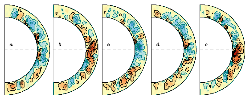
The horizontal spreading of a new upflow is limited by interactions with adjacent convection cells and by the need to transport heat outward and ultimately through the boundary, as discussed by Rast (1995, 2003). As can be seen in Figure 11 (see also Fig. 2$a$), the strongest upflows occur adjacent to the downflow lanes. As a convection cell expands horizontally, the upward flow at the center of the cell drops, leading to a reduction in the outward enthalpy flux. Cooling of the fluid due to the upper boundary condition eventually reverses the buoyancy driving, thus forming a new downflow lane which bisects and thereby fragments the existing convection cell. This occurs continually in our simulation as demonstrated in Figure 11 (C). Similar dynamics also occur at lower latitudes, as can be seen by careful scrutiny of Figure 9. Such fragmentation induced by cooling near the upper boundary is the principle factor in determining the size and lifetime of the cells which make up the downflow network.

Convection cells may also be squeezed out of existence, or collapse, via the horizontal spreading of adjacent cells as illustrated in Figure 11 (D). Shearing of convection cells by differential rotation also limits their lifetime and horizontal scale. Such processes typically occur over the course of several days but some convection cells can persist with little distortion for nearly a week (Fig. 11, E).

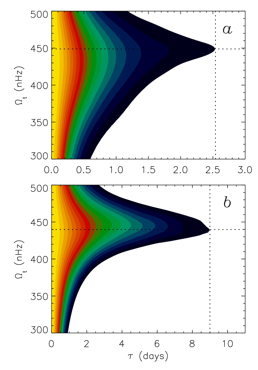
A quantitative measure of the lifetime and propagation rate of convective patterns can be obtained by considering the autocorrelation function, acf, defined as follows:

$$\mbox{acf}(r,t,\Omega_{t},\tau)=\\ \frac{\int_{\theta_{1}}^{\theta_{2}}\int_{0}^{2\pi}v_{r}(r,\theta,\phi,t)v_{r}(r,\theta,\phi-\Omega_{t}\tau,t+\tau)\sin\theta d\theta d\phi}{\int_{\theta_{1}}^{\theta_{2}}\int_{0}^{2\pi}v_{r}^{2}(r,\theta,\phi,t)\sin\theta d\theta d\phi}$$ (16)

where $\Omega_{t}$ is the tracking rate (expressed as an angular velocity), $\tau$ is the temporal lag and $\theta_{1}$ and $\theta_{2}$ specify the desired latitudinal band (averaged over the northern and southern hemispheres). Results are illustrated in Figure 12.

Figure 12.— The acf is shown as a function of tracking rate $\Omega_{t}$ and lag $\tau$ for latitude band 0^∘-20^∘ at ($a$) $r=0.98R$ and ($b$) $r=0.85R$. For each tracking rate, the acf drops from a value of unity (yellow) to zero (white) with contour levels spaced at intervals of 0.05. Dotted lines indicate the the optimal tracking rate and the associated correlation time.

Table 1Correlation times and Optimal Tracking Rates

	radius	$0^{\circ}$–$20^{\circ}$	$20^{\circ}$–$40^{\circ}$	$40^{\circ}$–$60^{\circ}$	$60^{\circ}$–$90^{\circ}$
$\Omega$ (nHz)	0.98$R$	414-421	421-408	408-375	375-358
$\Omega_{c}$ (nHz)	0.98$R$	450	430	380	330
$\tau_{c}$ (days)	0.98$R$	2.6	2.0	2.0	2.2
$\Omega$ (nHz)	0.85$R$	429-415	415-400	400-372	372-358
$\Omega_{c}$ (nHz)	0.85$R$	440	424	400	390
$\tau_{c}$ (days)	0.85$R$	9.0	8.2	8.0	8.0

The acf is unity at $\tau=0$ and drops monotonically with increasing lag. For each value of $\Omega_{t}$ one may define a correlation time as the time beyond which the acf drops below a fiducial threshold, here taken to be 0.05. We then define an optimal tracking rate $\Omega_{c}$ as that value of $\Omega_{t}$ which maximizes the correlation time, $\tau_{c}$. Optimal rates and correlation times for various latitude bands are listed in Table 1. Also listed for comparison is the variation of the mean rotation rate $\Omega$ across each latitude band for the radius and time interval used to compute the acf.

The acf in Figure 12$a$ corresponds to low-latitude convective patterns near the surface, such as in Figure 9. Here the flow is dominated by the intricate, continually evolving downflow network and correlation times are only a few days. The maximum correlation time of 2.6 days is achieved with a tracking rate of 450 nHz which corresponds to the propagation rate of the NS downflow lanes as indicated by the arrow in Figure 9. These NS downflow lanes are the longest-lived structures within the downflow network and they propagate faster than the mean rotation rate of 414-421 nHz (Table 1). Thus, they are propagating convective modes as opposed to passive features being advected by the differential rotation.

The NS downflow lanes are more prominent deeper in the convection zone and this is reflected in the acf of Figure 12$b$. The acf is more strongly peaked at the optimal tracking rate and the associated correlation time is longer, $\tau_{c}$ = 9.0 days. At 440 nHz, $\Omega_{t}$ is somewhat less at $r=0.85R$ than at $r=0.98R$ but it is still faster than the local rotation rate (Table 1).

The prograde propagation of NS downflow lanes can be attributed to the approximate local conservation of potential vorticity, and in this sense they may be regarded as thermal Rossby waves (Busse, 1970; Glatzmaier & Gilman, 1981b). NS downflow lanes are related to banana cells and columnar convective modes that occur in more laminar, more rapidly rotating, and more weakly stratified systems and that have been well studied both analytically and numerically (reviewed by Zhang & Schubert, 2000; Busse, 2002). In general, their propagation rate depends on the rotation rate, the stratification, and the geometry of the shell.

Figure 13.— Power spectra plotted as a function of spherical harmonic degree $\ell$, summed over all orders $m>0$ and averaged over a time interval of 62 days. Solid and dotted lines sample spherical surfaces $r=0.98R$ and $r=0.92R$ respectively. Quantities include ($a$-$c$) the velocity components, ($d$) the horizontal divergence, ($e$) the vertical vorticity, and ($f$) the temperature fluctuations.

At mid latitudes, the correlation times are somewhat smaller and the optimal tracking rates are slower, comparable to the local rotation rate (Table 1). Near the poles $\Omega$ and $\Omega_{t}$ become less reliable because the small momentum arm induces large temporal variations in angular velocity. Linear theory indicates that polar convective modes should propagate slowly retrograde (Gilman, 1975; Busse & Cuong, 1977) but it is uncertain whether such linear modes persist in this highly nonlinear parameter regime. Correlation times at high latitudes are comparable to those at mid latitudes, about two days for the downflow network in the upper convection zone and about 8 days for the larger-scale flows in the mid convection zone.

We emphasize that statistical measures such as $\tau_{c}$ can drastically underestimate the lifetime of coherent structures within a turbulent flow such as this. It is evident from Figures 9 and 10 that some NS downflow lanes persist for weeks and even months. Likewise, some higher-latitude convective cells at $r=0.98R$ can persist for up to a week (e.g. Fig. 11, E).

6. Horizontal Spectra and Length Scales

In §3 we discussed the convective patterns realized in our simulations and in §5 we described their temporal evolution. In this and the following section we consider univariate and bivariate statistics in order to gain further insight into the nature of the convective flows. Throughout this analysis we will be concerned solely with fluctuating quantities ($m>0$), indicated by primes. The structure and evolution of mean flows is discussed in §4. Furthermore, we focus on the upper portion of the convection zone which is most relevent to local helioseismology.

Figure 14.— Probability density functions (pdfs) are shown for ($a$) $v_{r}^{\prime}$, ($b$) $v_{\theta}^{\prime}$, ($c$) $v_{\phi}^{\prime}$, ($d$) $\Delta^{\prime}$, ($e$) $\zeta^{\prime}$, and ($f$) $T^{\prime}$. The pdfs shown correspond to spherical surfaces at $r=0.98R$ (solid lines) and $r=0.92$ (dotted lines) and are averaged over time (62 days). Moments of the fluctuating velocity pdfs as a function of depth are shown in Fig. 15.

Figure 13 shows the spherical harmonic spectra of the velocity and temperature fields at two levels in the upper convection zone as a function of spherical harmonic degree $\ell$, which may be regarded as the total horizontal wavenumber. At $r=0.98R$, the radial velocity spectrum (Fig. 13$a$) increases with $\ell$ approximately as $\ell^{3}$, reaching a maximum at $\ell\sim 80$. Afterward it drops with a best-fit exponent of $n\approx-5$, where the power $P(\ell)\propto\ell^{n}$.

The spherical harmonic degree $\ell=80$ corresponds to a horizontal scale $L$ of 54 Mm, which may be regarded as a characteristic scale of the downflow network illustrated in Figures 1$a$ and 4$a$ and in the upper row of Figure 2$a$. However, a single characteristic scale is somewhat misleading as the downflow network exhibits structure on a vast range of scales. A look at the convective patterns in Figure 11, for example, reveals convection cells 10^∘-20^∘ (100-200 Mm) across as well as cyclonic vortices spanning only a few degrees (10-30 Mm). Meanwhile, NS downflow lanes can extend to latitudes of $\pm 25^{\circ}$ or more, spanning more than 500 Mm (e.g. Fig. 10).

Deeper in the convection zone, the convective scales are generally larger. The radial velocity spectrum at $r=0.92$ peaks at $\ell=26$, corresponding to a horizontal scale of about 150 Mm (Fig. 13$a$, dotted line). Furthermore, the high-$\ell$ dropoff in power is somewhat steeper than at $r=0.98R$, with an exponential providing a better fit than a polynomial; $P(\ell)\propto\exp\left(\alpha\ell\right)$, with $\alpha=-0.015$.

The horizontal velocity spectra peak at $\ell$ = 10-20 ($L\sim$ 200-400 Mm) for both radial levels sampled in Figure 13$b$, $c$. These scales are larger than for the radial velocity as a consequence of mass conservations. Near the impenetrable boundary, the radial velocity is highly correlated with the horizontal divergence such that $v_{r}\sim\Delta\sim\ell v_{h}$ where $v_{h}$ is the horizontal velocity. The $v_{\theta}^{\prime}$ and $v_{\phi}^{\prime}$ spectra are thus somewhat flatter than $v_{r}^{\prime}$ at high $\ell$ ($n\approx-4.6$). At $r=0.92R$, the $v_{\theta}^{\prime}$ and $v_{\phi}^{\prime}$ spectra, like the $v_{r}^{\prime}$ spectrum, are best fit by exponentials with $\alpha\sim-0.016$.

The correspondence between the radial velocity $v_{r}$ and the horizontal divergence $\Delta$ near the upper boundary is apparent when comparing frames $a$ and $d$ of Figure 13. At $r=0.98R$ the two spectra are nearly identical when normalized by their maximum value. By $r=0.92$ differences become significant, with the $\Delta^{\prime}$ spectrum shifted toward higher wavenumber relative to the $v_{r}^{\prime}$ spectrum.

The vertical vorticity spectra in Figure 13$e$ peak at even higher wavenumber, $\ell=140$ ($L\sim$ 30 Mm) at $r=0.98$. This reflects the presence of the high-latitude cyclones discussed in (§3) which are highly intermittent in space and time. Beyond this maximum, the $\zeta^{\prime}$ spectrum decays approximately as $\ell^{-2}$. Deeper in the convection zone at $r=0.92R$, the peak shifts toward lower wavenumber ($\ell\sim 100$, $L\sim 40$ Mm) and the spectrum steepens ($n\sim-4$).

The spectrum of temperature fluctuations is flatter than the velocity field at low $\ell$, with a broad maximum at $\ell\sim 16$ (260 Mm). This reflects the low Prandtl number and the large-scale thermal variations associated with thermal wind balance (§4). The slope at high $\ell$ is comparable to the velocity field, with $n\sim-4.2$ at $r=0.98$ and $\alpha\sim-0.019$ at $r=0.92R$.

Figure 15.— The ($a$) standard deviation, ($b$) skewness, and ($c$) kurtosis of the three velocity components are shown as a function of radius, averaged over a time interval of 62 days. The solid, dotted, and dashed lines represent $v_{r}^{\prime}$, $v_{\theta}^{\prime}$ and $v_{\phi}^{\prime}$ respectively. Horizontal dashed lines show skewness and kurtosis values for a Gaussian distribution (${\cal S}=0$, ${\cal K}=3$) for comparison.

7. Probability Density Functions and Moments

More detailed information about the nature of the flow field may be obtained from probability density functions (pdfs) as shown in Figure 14. These are normalized histograms on horizontal surfaces which take into account the spherical geometry. The shape of a pdf $f(x)$ may be described through its moments of order $n$, defined as

$${\cal M}^{n}=\int\left(x-\left<x\right>\right)^{n}f(x)dx\\ =\frac{1}{4\pi}\int_{0}^{\pi}\int_{0}^{2\pi}\left(x-\left<x\right>\right)^{n}\sin\theta~{}d\theta~{}d\phi~{}~{}~{}.$$ (17)

We then define the standard deviation $\sigma$, the skewness ${\cal S}$, and the kurtosis ${\cal K}$ as follows: $\sigma=({\cal M}^{2})^{1/2}$, ${\cal S}={\cal M}^{3}\sigma^{-3}$, and ${\cal K}={\cal M}^{4}\sigma^{-4}$. Results are illustrated in Figure 15 as a function of radius.

Near the top of the convection zone, the radial velocity pdf exhibits a bimodal structure, with two distinct maxima at positive and negative $v_{r}$ (Fig. 14$a$, solid line). These maxima suggest characteristic velocity scales of $\sim 6$ m s^-1 for upflows and $\sim 30$ m s^-1 for downflows. However, these values are substantially smaller than the standard deviation (rms value) of $v_{r}^{\prime}$ which peaks at 160 m s^-1 at $r=0.96R$ and then drops to zero at the upper boundary (Fig. 15$a$).

The larger amplitude of the positive peak reflects the larger filling factor of upflows relative to downflows. By $r=0.92R$, the negative peak has largely disappeared and the negative tail of the pdf becomes nearly exponential (dotted line). This signifies turbulent entrainment, whereby much of the momentum of downflow lanes and plumes is transferred to the surrounding fluid and dispersed. The asymmetry between narrow, stronger downflows and broader, weaker upflows is a consquence of the density stratification (§3) and is manifested as a large negative skewness which persists throughout the convection zone (Fig. 15$b$).

The kurtosis ${\cal K}$ is generally regarded as a measure of spatial intermittency but large values can also arise from bimodality. A unimodal Gaussian distribution yields ${\cal K}=3$ whereas an exponential distribution yields ${\cal K}=6$. The $v_{r}^{\prime}$ pdf has an even larger kurtosis ranging from 3-12 across the convection zone (Fig. 15$c$), reflecting both intermittency and bimodality.

By comparison, the horizontal velocity pdfs shown in Figure 14$b$, $c$ appear more symmetric with nearly exponential tails (${\cal K}=$ 3-5; Fig. 15$c$). The positive skewness of the $v_{\phi}^{\prime}$ pdf is a signature of the NS downflow lanes discussed in §3 and §5. Their north-south orientation and prograde propagation implies converging zonal flows in which the eastward velocities on the trailing edge of the lanes are somewhat faster on average than the westward velocities on the leading edge.

Velocity amplitudes increase with radius due to the density stratification, with horizontal velocity scales reaching over 200 m s^-1 near the surface (Fig. 15$a$). In the mid convection zone the velocity field is nearly isotropic, with a characteristic amplitude of about 100 m s^-1 for all three components.

The horizontal divergence pdf shown in Figure 14$d$ is nearly identical to the $v_{r}^{\prime}$ pdf in Figure 14$a$ at $r=0.98$, but as with the spectra in Figure 13$d$, this correspondence breaks down by $r=0.92R$. In the mid-convection zone the $\Delta$ pdf becomes more symmetric with nearly exponential tails (${\cal S}$ = -0.13, ${\cal K}$ = 9.2 at $r=0.92R$). Non-Gaussian behavior such that ${\cal K}>3$ for velocity differences and derivatives is a well-known feature found in a wide variety of turbulent flows (e.g. Chen et al., 1989; Castaing et al., 1990; She, 1991; Kailasnath et al., 1992; Miesch et al., 1999; Jung & Swinney, 2005; Bruno & Carbone, 2005). In particular, the pdf of velocity differences between two points separated in space is often modeled using stretched exponentials $f(x)\propto\exp(-|x|^{\beta})$, where $\beta$ approaches unity for small spatial separations (as sampled by derivatives) and becomes more Gaussian ($\beta\approx 2$) as the spatial separation increases.

The vertical vorticity pdfs shown in Figure 14$e$ also exhibit nearly exponential tails. However, near the surface ($r=0.98R$) the distribution is bimodal with prominent tails signifying an abundance of extreme events (${\cal K}=180$). These tails arise from the intense, intermittent cyclones which develop at the intersticies of the downflow network at mid and high latitudes as discussed in §3. By $r=0.92R$, the bimodality is absent, although the pdf is still highly intermittent (${\cal K}=25$). This is consistent with Figure 2$b$ which suggests that the high-latitude cyclones are confined to the outer few percent of the convection zone ($r\gtrsim 0.95R$).

The signature of high-latitude cyclones is also present in the pdf of temperature fluctuations as a prominent exponential tail on the negative side at $r=0.98R$ (Fig. 14$f$). As with the radial velocity pdf, the bimodality disappears by $r=0.92R$ due to entrainment and the negative tail becomes unimodal and exponential. The asymmetric shape of the tempature pdfs arises from the asymmetric nature of the convection noted in §3; cool downflows are generally less space-filling and more intense than warm upflows. The temperature pdfs remain asymmetric (${\cal S}<0$) and intermittent (${\cal K}>3$) throughout the convection zone, becoming most extreme near the surface where ${\cal S}=-1.6$ and ${\cal K}=12$. The standard deviation of the temperature fluctuations ranges from 0.4 K in the lower convection zone to a maximum of 4 K at $r=0.96R$.

Figure 16.— Correlations between $v_{\theta}^{\prime}$–$v_{\phi}^{\prime}$ (left column), $\zeta^{\prime}$–$\Delta^{\prime}$ (middle column), and $v_{r}^{\prime}$–$T^{\prime}$ (right column) are shown at $r=0.98$. ($a$)–($i$) 2–D pdfs averaged over a time interval of 62 days (yellow denotes the maximum contour level). Results are shown for latitude bands of $0^{\circ}$–$30^{\circ}$ ($g$–$i$), $30^{\circ}$–$60^{\circ}$ ($d$–$f$), and $60^{\circ}$–$90^{\circ}$ ($a$–$c$), averaged over the northern and southern hemispheres (reversing the sign of $v_{\theta}^{\prime}$ and $\zeta^{\prime}$ in the southern hemisphere). ($j$)–($l$) mean correlations, obtained by vertically averaging the 2–D histograms (pdfs) in each horizontal bin. Red, black, and blue lines represent low ($0^{\circ}$–$30^{\circ}$), mid ($30^{\circ}$–$60^{\circ}$), and high ($60^{\circ}$–$90^{\circ}$) latitudes respectively.

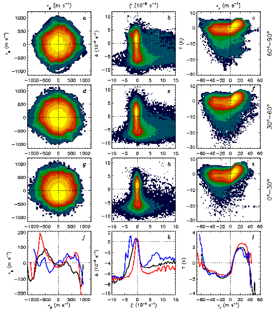
Correlations between vertical velocity and temperature fluctuations may be investigated further by means of two-dimensional pdfs (histograms) as illustrated in Figure 16 for $r=0.98R$. Although warmer and cooler temperatures are associated with upflows and downflows respectively, the relationship is not linear. Upflows exhibit a prominent maximum at $v_{r}^{\prime}\sim 20$ m s^-1 and $T^{\prime}\sim 2$ K, whereas downflows are more distributed, both in the range of velocity amplitudes and in the spread of temperature variations for a given $v_{r}^{\prime}$. This spread increases somewhat toward higher latitudes due to the preponderence of intermittent cyclonic plumes but the average correlation shown in Figure 16$l$ is insensitive to latitude. The reversal in the sense of the temperature variation at high radial velocity amplitudes is due in part to poor statistics (few events) but it does have physical implications. As noted in §3, the strongest upflows occur adjacent to downflow lanes. Cool regions associated with downflow lanes tend to be more diffuse than the lanes themselves as a result of the low Prandtl number ($P_{r}=0.25$). Thus, the fastest upflows can be relatively cool. Similarly, the fastest downflows occur in localized regions adjacent to warmer upflows such that the temperature fluctuations are diminished by thermal diffusion.

Correlations between the horizontal velocity components $v_{\theta}^{\prime}$ and $v_{\phi}^{\prime}$ are of particular interest because these may be compared with analogous correlations obtained from local helioseismology. Such correlations not only represent a potential diagnostic for giant-cell convection, but they also reflect latitudinal angular momentum transport by Reynolds stresses which plays an essential role in maintaining the differential rotation profile (§4). However, the 2-D pdfs in Figure 16$a$, $d$, and $g$ appear nearly isotropic, implying that the horizontal velocity components near the surface ($r=0.98R$) are only weakly correlated. At high latitudes, there is a weak positive correlation signifying equatorward angular momentum transport, but at mid-latitudes the sense of the correlation reverses (Fig. 16$j$). At low latitudes there is no clear systematic behavior, as expected if horizontal velocity correlations are induced by the vertical component of the rotation vector.

The lack of prominent horizontal velocity correlations in the near-surface downflow network may be attributed to the relatively small spatial and temporal scales of the convection. The effective Rossby number here is greater than for the larger-scale motions deeper in the convection zone, implying weaker rotational influence (§2.2). Coriolis-induced correlations are consequently weaker. Since the differential rotation is maintained primarily by horizontal Reynolds stresses (§4), weaker horizontal velocity correlations help account for the decrease in latitudinal shear found in our simulation near the outer boundary. A near-surface shear layer is also found in helioseismic inversions, but in that case there is nearly uniform acceleration of the angular velocity at all latitudes so the latitudinal shear does not change significantly (Thompson et al., 2003). As discussed in §4, mean flows in the uppermost portion of the convection zone are likely sensitive to the subtle dynamics of the surface boundary layer and may require more sophisticated modeling approaches to capture fully. If a decrease in horizontal velocity correlations does indeed occur near the surface of the Sun as suggested by our simulations, then such correlations may be difficult to detect in helioseismic inversions.

A more promising diagnostic to search for in SSW maps may be correlations between horizontal divergence and vertical vorticity. Although there is much scatter, Figure 16 ($b$, $e$, $h$) demonstates a clear correlation between cyclonic vorticity and horizontal convergence which becomes more prominent at higher latitudes. This correlation is a signature of the Coriolis force as described in §3. There is also a correlation between anticyclonic vorticity and horizontal divergence but this only occurs for small values of $\zeta$. The most intense vorticity of both signs occurs in regions of horizontal convergence. This is consistent with the interpretation discussed in §3 in which downflow lanes are generally more turbulent than upflows. Vorticity of all orientations is generated by shear and entrainment and amplified by vortex stretching.

Komm et al. (2007) have presented evidence for correlations between $\zeta^{\prime}$ and $\Delta^{\prime}$ in SSW maps derived from SOHO/MDI and GONG data. These correlations are approximately linear in regions of low magnetic activity, with cyclonic and anti-cyclonic vorticity associated with horizontal convergence and divergence respectively. This is qualitatively consistent with our simulation results since the high-amplitude anticyclonic vorticity in our simulations is associated with localized features which would be filtered out by the spatial averaging inherent in the helioseismic inversions. A more detailed comparison between our simulation results and SSW maps will be carried out in a subsequent paper.

8. Summary and Conclusions

High-resolution simulations of turbulent convection provide essential insight into the nature of global-scale motions in the solar convection zone, often referred to as giant cells, and into how these motions maintain the solar differential rotation and meridional circulation. Such insight is essential to inspire and interpret investigations of solar interior dynamics based on helioseismic inversions and photospheric observations. Although the simulation we focus on here is non-magnetic, our results have important implications for solar dynamo theory and may be used to assess, calibrate, and further develop other modeling strategies such as mean-field models of solar and stellar activity cycles.

The convective patterns realized in our simulations are intricate and continually evolving. Near the top of our computational domain at $r=0.98R$, there is an interconnected network of downflow lanes reminiscent of photospheric granulation but on a much larger scale. The power spectrum of the radial velocity peaks at $\ell\sim 80$, corresponding to a horizontal scale of about 50 Mm. However, a visual inspection of the convective patterns (Figs. 1, 2, 4, 11) reveals a wide range of scales, with many cells spanning $10^{\circ}$-20^∘ (100-200 Mm). Characteristic horizontal velocity scales are 250 m s^-1 at $r=0.98R$, dropping to $\sim 100$ m s^-1 in the mid convection zone. Near the surface, zonal flow amplitudes ($v_{\phi}^{\prime}$) are on average about 10% larger than latitudinal flow amplitudes ($v_{\theta}^{\prime}$) but in the mid convection zone all three velocity components have a comparable amplitude. Deep in the convection zone the surface network fragments into disconnected downflow lanes and plumes but the skewness of the radial velocity remains strongly negative (Fig. 15$b$).

A close inspection of the downflow network near the surface reveals a distinct tendency for structures to align in a north-south orientation at low latitudes. Such NS downflow lanes represent the largest and longest-lived features in the convection zone. Whereas correlation time scales for the downflow network are only a few days, NS downflow lanes can persist for weeks or even months. They are traveling convective modes which propagate in longitude about 8% faster than the equatorial rotation rate. Near the bottom of the shell the lanes fragment into downwelling plumes but some coherence extends across the entire convection zone (e.g. Fig. 4).

At higher latitudes, the downflow network is more isotropic and possesses intense cyclonic vorticity, induced by Coriolis forces. Localized cyclonic vortices are prevalent near the interstices of the network at latitudes above about $\pm 30^{\circ}$. These structures are similar to the turbulent helical plumes observed by Brummell et al. (1996) in Cartesian $f$-plane simulations and are associated with downward flow, horizontal convergence, and cool temperatures as well as cyclonic radial vorticity. They are confined to the upper convection zone ($r\gtrsim 0.95R$) and their horizontal scale is comparable to that of supergranulation, about 10-30 Mm. Typical lifetimes are several days to a week (e.g. Fig. 11). High-latitude cyclones are highly intermittent and give rise to prominent exponential tails in the radial vorticity and temperature pdfs (Fig. 14).

Near the surface, the horizontal divergence $\Delta^{\prime}$ is highly correlated with the radial velocity $v_{r}^{\prime}$. Thus, horizontal divergence fields obtained from SSW maps should provide a good proxy for the radial velocity, at least on large scales. Furthermore, there is a strong correlation between $\Delta^{\prime}$ and the radial vorticity $\zeta^{\prime}$, with intense cyclonic vorticity in regions of horizontal convergence (downflows) amid a background of weaker anticyclonic vorticity in broader regions of divergence (upflows). This correlation applies over most of the horizontal surface area but breaks down for localized, high-amplitude events; the most intense vorticies, both cyclonic and anticyclonic, occur in downflow lanes ($\Delta^{\prime}<0$). Correlations between $\zeta^{\prime}$ and $\Delta^{\prime}$ represent a promising diagnostic for the investigation of large-scale flow patterns in SSW maps (Komm et al., 2007).

A significant new feature of the simulation presented here relative to previous models is the manner in which the differential rotation is maintained. As demonstrated in Figure 7, the resolved convective motions transport angular momentum equatorward and inward by means of Reynolds stresses while the meridional circulation opposes this transport, such that

$$\mbox{\boldmath$\nabla\mbox{\boldmath$\cdot$}$}\overline{\left({\bf F}^{RS}+{\bf F}^{MC}\right)}\approx 0~{}~{}~{}.$$ (18)

This simulation has thus crossed a threshold in which viscous diffusion ${\bf F}^{VD}$ no longer contributes significantly to the angular momentum balance.

The implications of this result are profound. Although there are subtle nonlinear feedbacks, the meridional circulation pattern is largely determined by ${\bf F}^{RS}$ under the constraint that the resulting mean flows satisfy equation (18). Convective motions (particularly NS downflow lanes) redistribute angular momentum and the resulting differential rotation induces circulations through Coriolis forces until a steady state is reached. Baroclinicity also plays an important role, breaking the Taylor-Proudman constraint which favors cylindrical rotation profiles. Baroclinic torques arise in part from thermal coupling to the tachocline which is represented in our simulation by imposing a latitudinal entropy gradient on the lower boundary at the base of the convection zone (§2.2).

The mean flows which result are similar to those inferred from helioseismic inversions. The mean angular velocity decreases monotonically with latitude with nearly radial contours at mid-latitudes. This is similar to the solar rotation profile, although the angular velocity contrast of $\sim$ 50 nHz between 0^∘-60^∘ is smaller than the $\sim$ 90 nHz in the Sun (Thompson et al., 2003). The time-averaged meridional circulation is dominated by a single cell in each hemisphere with poleward flow of about 20 m s^-1 in the upper convection zone (notwithstanding a flow reversal near the upper boundary which may be artificial). The sense and amplitude of this circulation is comparable to that inferred near the surface of the Sun from Doppler measurements and helioseismic inversions. The lower convection zone currently lies beyond the reach of helioseismic probing but many have proposed that an equatorward return flow may exist and furthermore that this global circulation pattern may play an essential role in establishing the solar activity cycle (Dikpati & Charbonneau, 1999; Dikpati et al., 2004, e.g.). For a review of these so-called flux-transport dynamo models, see Charbonneau (2005). The mean meridional circulation in our simulation is similar to that used in many flux-transport dynamo models but month-to-month fluctuations about this mean are large.

In order to gain further insight into how the global solar dynamo operates and into how mean flows are maintained, we must extend the lower boundary of our computational domain below the solar convection zone and thus explicitly resolve the complex dynamics occurring in the overshoot region and tachocline. Furthermore, we must incorporate magnetism and investigate how magnetic flux is amplified, advected, and organized by turbulent penetrative convection, rotational shear, and global circulations. Such efforts are already underway (Browning et al., 2006) and will continue. Future work will also focus on improving our understanding of the upper convection zone, including how granulation and supergranulation influence giant cells and mean flow patterns, and how signatures of internal flows and magnetism might be manifested in helioseismic measurements and photospheric observations.

References

- Brandenburg et al. (1996) Brandenburg, A., Jennings, R. L., Nordlund, A., Rieutord, M., Stein, R. F., & Tuominen, I. 1996, J. Fluid Mech., 306, 325
- Braun & Fan (1998) Braun, D. C. & Fan, Y. 1998, ApJ, 508, L105
- Browning et al. (2006) Browning, M. K., Miesch, M. S., Brun, A. S., & Toomre, J. 2006, ApJ, 648, L157
- Brummell et al. (1996) Brummell, N. H., Hurlburt, N. E., & Toomre, J. 1996, ApJ, 473, 494
- Brun et al. (2004) Brun, A. S., Miesch, M. S., & Toomre, J. 2004, ApJ, 614, 1073
- Brun & Toomre (2002) Brun, A. S. & Toomre, J. 2002, ApJ, 570, 865
- Bruno & Carbone (2005) Bruno, R. & Carbone, V. 2005, Living Reviews in Solar Physics, 2, online journal, http://www.livingreviews.org/lrsp-2005-5
- Busse (1970) Busse, F. H. 1970, J. Fluid Mech., 44, 441
- Busse (2002) —. 2002, Phys. Fluids, 14, 1301
- Busse & Cuong (1977) Busse, F. H. & Cuong, P. G. 1977, Geophys. Astrophys. Fluid Dyn., 8, 17
- Canuto et al. (1994) Canuto, V. M., Minotti, F. O., & Schilling, O. 1994, ApJ, 425, 303
- Castaing et al. (1990) Castaing, B., Gagne, Y., & Hopfinger, E. J. 1990, Physica D, 46, 177
- Charbonneau (2005) Charbonneau, P. 2005, Living Reviews in Solar Physics, 2, online journal, http://www.livingreviews.org/lrsp-2005-2 (cited Jan 2007)
- Chen et al. (1989) Chen, H., Herring, J. R., Kerr, R. M., & Kraichnan, R. H. 1989, Phys. Fluids A, 1, 1844
- Christensen-Dalsgaard et al. (1996) Christensen-Dalsgaard, J. et al. 1996, Science, 272, 1286
- Clune et al. (1999) Clune, T. C., Elliott, J. R., Miesch, M. S., Toomre, J., & Glatzmaier, G. A. 1999, Parallel Computing, 25, 361
- Covas et al. (2000) Covas, E., Tavakol, R., Moss, D., & Tworkowski, A. 2000, A&A, 360, L21
- Dikpati & Charbonneau (1999) Dikpati, M. & Charbonneau, P. 1999, ApJ, 518, 508
- Dikpati et al. (2004) Dikpati, M., de Toma, G., Gilman, P. A., Arge, C. N., & White, O. R. 2004, ApJ, 601, 1136
- Elliott et al. (2000) Elliott, J. R., Miesch, M. S., & Toomre, J. 2000, ApJ, 533, 546
- Gilman (1975) Gilman, P. A. 1975, Journ. Atmos. Sci., 32, 1331
- Gizon & Birch (2005) Gizon, L. & Birch, A. C. 2005, Living Reviews in Solar Physics, 2, online Journal article, http://www.livingreviews.org/lrsp-2005-6
- Glatzmaier & Gilman (1981a) Glatzmaier, G. A. & Gilman, P. A. 1981a, ApJS, 45, 351
- Glatzmaier & Gilman (1981b) —. 1981b, ApJS, 45, 381
- González-Hernandez et al. (2006) González-Hernandez, I., Komm, R., Hill, F., Howe, R., Corbard, T., & Haber, D. A. 2006, ApJ, 638, 576
- Gough (1969) Gough, D. O. 1969, J. Atmos. Sci., 26, 448
- Haber et al. (2002) Haber, D. A., Hindman, B. W., & Toomre, J. 2002, ApJ, 570, 855
- Haber et al. (2004) Haber, D. A., Hindman, B. W., Toomre, J., & Thompson, M. J. 2004, Solar Physics, 220, 371
- Hathaway (1996) Hathaway, D. H. 1996, ApJ, 460, 1027
- Hathaway et al. (2000) Hathaway, D. H., Beck, J. G., Bogart, R. S., Bachmann, K. T., Khatri, G., Petitto, J. M., Han, S., & Raymond, J. 2000, Solar Physics, 193, 299
- Hindman et al. (2004) Hindman, B. W., Gizon, L., T. L. Duvall, J., Haber, D. A., & Toomre, J. 2004, ApJ, 613, 1253
- Hindman et al. (2006) Hindman, B. W., Haber, D. A., & Toomre, J. 2006, ApJ, 653, 725
- Jung & Swinney (2005) Jung, S. W. & Swinney, H. L. 2005, Phys. Rev. E, 72, 026304
- Kailasnath et al. (1992) Kailasnath, P., Sreenivasan, K. R., & Stolovitzky, G. 1992, Phys. Rev. Lett., 68, 2766
- Kitchatinov & Rüdiger (1993) Kitchatinov, L. L. & Rüdiger, G. 1993, A&A, 276, 96
- Kitchatinov & Rüdiger (2005) —. 2005, Astron. Nachr., 326, 379
- Komm et al. (2007) Komm, R., Howe, R., Hill, F., Miesch, M., Haber, D., & Hindman, B. 2007, ApJ, submitted
- Komm et al. (2004) Komm, R. W., Corbard, T., Durney, B. R., González-Hernández, I., Hill, F., Howe, R., & Toner, C. 2004, ApJ, 605, 554
- Komm et al. (1993) Komm, R. W., Howard, R. F., & Harvey, J. W. 1993, Solar Physics, 147, 207
- Komm et al. (2005) Komm, R. W., Howe, R., Hill, F., González-Hernández, I., Toner, C., & Corbard, T. 2005, ApJ, 631, 636
- Lantz & Fan (1999) Lantz, S. R. & Fan, Y. 1999, ApJ, 121, 247
- Miesch (2005) Miesch, M. S. 2005, Living Reviews in Solar Physics, 2, online journal, http://www.livingreviews.org/lrsp-2005-1 (cited Jan 2007)
- Miesch et al. (2006) Miesch, M. S., Brun, A. S., & Toomre, J. 2006, ApJ, 641, 618
- Miesch et al. (2000) Miesch, M. S., Elliott, J. R., Toomre, J., Clune, T. C., Glatzmaier, G. A., & Gilman, P. A. 2000, ApJ, 532, 593
- Miesch et al. (1999) Miesch, M. S., Scalo, J. M., & Bally, J. 1999, ApJ, 524, 895
- Porter & Woodward (2000) Porter, D. H. & Woodward, P. R. 2000, ApJS, 321, 323
- Rast (1995) Rast, M. P. 1995, ApJ, 443, 863
- Rast (2003) —. 2003, ApJ, 597, 1200
- Rempel (2005) Rempel, M. 2005, ApJ, 622, 1320
- Rempel (2007) —. 2007, ApJ, 655, 651
- Rüdiger et al. (2005) Rüdiger, G., Egorov, P., & Ziegler, U. 2005, Astron. Nachr., 326, 315
- She (1991) She, Z.-S. 1991, Fluid Dynamics Research, 8, 143
- Spruit (2003) Spruit, H. C. 2003, Solar Physics, 213, 1
- Stein & Nordlund (1998) Stein, R. F. & Nordlund, A. 1998, ApJ, 499, 914
- Tassoul (1978) Tassoul, J. L. 1978, Theory of Rotating Stars (Princeton: Princeton Univ. Press)
- Thompson et al. (2003) Thompson, M. J., Christensen-Dalsgaard, J., Miesch, M. S., & Toomre, J. 2003, ARA&A, 41, 599
- Toomre (2002) Toomre, J. 2002, Science, 296, 64
- Zahn (1992) Zahn, J.-P. 1992, A&A, 265, 115
- Zhang & Schubert (2000) Zhang, K. & Schubert, G. 2000, ARA&A, 32, 409
- Zhao & Kosovichev (2004) Zhao, J. & Kosovichev, A. G. 2004, ApJ, 603, 776