CERN-PH-TH/2007-104

DFF 436/07/07

July 2007

A matrix formulation for small-$\boldsymbol{x}$ singlet evolution

M. Ciafaloni^(a), D. Colferai^(b), G.P. Salam^(c) and A.M. Staśto^(d)

^(a) CERN, Department PH-TH, CH-1211 Geneva 23, Switzerland
^(b) Dipartimento di Fisica, Università di Firenze, 50019 Sesto Fiorentino (FI), Italy;
INFN Sezione di Firenze, 50019 Sesto Fiorentino (FI), Italy
^(c) LPTHE, Université P. et M. Curie – Paris 6, Université D. Diderot – Paris 7, CNRS UMR 7589, Paris, France
^(d) Department of Physics, Pennsylvania State University, University Park, 16802 PA, USA;
H. Niewodniczański Institute of Nuclear Physics, Kraków, Poland

We propose a matrix evolution equation in $(x,\boldsymbol{k})$-space for flavour singlet, unintegrated quark and gluon densities, which generalizes DGLAP and BFKL equations in the relevant limits. The matrix evolution kernel is constructed so as to satisfy renormalization group constraints in both the ordered and antiordered regions of exchanged momenta $\boldsymbol{k}$, and incorporates the known NLO anomalous dimensions in the $\overline{\mathrm{MS}}$ scheme as well as the NL$x$ BFKL kernel. We provide a hard Pomeron exponent and effective eigenvalue functions that include the $n_{f}$-dependence, and give also the matrix of resummed DGLAP splitting functions. The results connect smoothly with those of the single-channel approach. The novel $P_{qa}$ splitting functions show resummation effects delayed down to $x=10^{-4}$, while both $P_{ga}$ entries show a shallow dip around $x=10^{-3}$, similarly to the $gg$ single-channel results. We remark that the matrix formulation poses further constraints on the consistency of a BFKL framework with the $\overline{\mathrm{MS}}$ scheme, which are satisfied at NLO, but marginally violated by small $n_{f}/N_{c}^{2}$-suppressed terms at NNLO.

1 Introduction

Small-x QCD evolution, historically based on DGLAP [1] and BFKL [2] dynamics, has been widely investigated in the past years [3, 4, 5, 6, 7, 8, 9], leading to a better understanding of the two approaches just mentioned and to robust resummed predictions for the gluon density and splitting function [10, 11, 12, 13, 14, 15, 16, 17]. There is now a remarkable consensus [18] among various resummation approaches on the resulting gluon evolution kernel, and a satisfactory comparison of some of them to experimental data [15, 19].

The basic idea underlying the progress of the resummation approaches just mentioned, lies in the observation [10] that the BFKL kernel embodies an infinite number of subleading contributions which are collinear singular. These terms are parametrically large and need to be taken into account in order to achieve consistency with the renormalization group (RG). The techniques for incorporating such terms differ in detail according to the various authors, but lead eventually to similar results.

However, all approaches developed so far limit themselves to a consistent resummation scheme only for the evolution of the gluon density. The quark-sea contribution is obtained on the basis of $\boldsymbol{k}$-factorization of the $q\bar{q}$ dipole [5] in the DIS factorization scheme and/or by adding the $q\bar{q}$ contribution to the next-to-leading-$\log x$ (NL$x$) BFKL kernel. The main purpose of the present paper is to devise a resummed small-$x$ evolution scheme in a coupled matrix form, so as to treat gluons and quarks on the same footing and in a collinear factorization scheme which is as close as possible to a predetermined one, e.g. the $\overline{\mathrm{MS}}$ scheme.

Our matrix approach, in the collinear limit, has the advantage that it complies automatically with the matrix factorization of the integrated partonic densities in the singlet evolution, and thus is able to incorporate the known low-order anomalous dimensions for any value of $\omega=N-1$, the moment index. On the other hand, in the high-energy limit, the (gauge-invariant) unintegrated partonic densities are well defined by $\boldsymbol{k}$-factorization around different values of $\omega$. To be precise, the gluon unintegrated density is defined around $\omega=0$ and the quark around $\omega=-1$. Therefore, in the leading high energy region — that is around $\omega=0$ — we are able to include the known LL$x$+NL$x$ BFKL kernel in the gluon channel only, thus leaving the quark entries somewhat unconstrained from the $\boldsymbol{k}$-factorization standpoint.

Note however that assuming a BFKL framework in matrix form is a demanding requirement, because $\boldsymbol{k}$-factorization implies resummation formulae for the anomalous dimension matrix up to NL$x$ level. Therefore, incorporating both exact low-order anomalous dimensions (say, in the $\overline{\mathrm{MS}}$ scheme) and NL$x$ expressions (from the exact BFKL kernel) imposes on our matrix kernel some nontrivial consistency relations expressing the requirement that collinear and high-energy schemes do not conflict with each other. They are discussed in detail in the following, and we find that they are satisfied in the $\overline{\mathrm{MS}}$ scheme up to NLO level, while they are marginally violated at NNLO, by small terms in the $gq$ entry of relative order $n_{f}/N_{c}^{2}$. For this reason we restrict ourselves, in this paper, to the NLO-NL$x$ level. This means that, starting at NNLO, our splitting functions will be in some matrix scheme which is not the $\overline{\mathrm{MS}}$ scheme. Higher order effects on the scheme change have been studied in [14] and have been found to be comparable to renormalization scale uncertainties.

Besides the NLO-NL$x$ information mentioned above, we impose the general requirement of consistency with the renormalization group in both ordered and antiordered configurations of exchanged partonic momenta $\boldsymbol{k}$’s. This is best expressed in the $\gamma\leftrightarrow 1+\omega-\gamma$ symmetry of the kernel, where $\gamma$ is conjugated to $\log\boldsymbol{k}^{2}$. We enforce this symmetry by the so-called consistency constraint [20, 21, 22] which introduces an $\omega$-dependence in the (leading) kernel, so as to resum those parts [9] of the higher order BFKL kernels which are required by the RG. This procedure follows previous papers [10, 11] and is used in particular for the $gg$ matrix element of the kernel.

Despite all such requirements, there is a considerable ambiguity in our approach which is tied up to the matrix structure, because the $\gamma$ and $\omega$ dependences of the various matrix elements of the kernel are constrained only to a limited extent by the collinear and high-energy limits. We therefore introduce in sec. 2 some further requirements, mostly related to the pole structure of the kernel in the $\gamma$ and $\omega$ variables, by requiring it to have at most simple poles. This assumption is quite natural in the case of $\omega\rightarrow 0$ because of the BFKL limit, and follows by the $\omega$-expansion method [10] in the $\gamma\rightarrow 0$ case. The leading twist pole structure of the kernel at lowest order in $\alpha_{\mathrm{s}}$ is basically $\mathsf{K}\sim\Gamma_{0}\;\left[(1/\gamma)+1/(1+\omega-\gamma)\right]$, where $\Gamma_{0}$ denotes the LO DGLAP anomalous dimension matrix. The full kernel to second order in $\alpha_{\mathrm{s}}$ is constructed in secs. 2 and 3 according to the requirements stated above. It also contains running coupling effects at the scales suggested by the NL$x$ BKL kernel and by the RG.

In the frozen $\alpha_{\mathrm{s}}$ case we calculate in sec. 4 the resulting anomalous dimension matrix, and its eigenvalues $\gamma_{\pm}(\alpha_{\mathrm{s}},\omega)$. The leading eigenvalue at high energies, $\gamma_{+}$, contains important resummation effects in the $\alpha_{\mathrm{s}}/\omega$ variable. We also obtain resummation formulae for $\Gamma_{qg}$ and $\Gamma_{gq}$, the latter being specific to our matrix approach and not directly obtained on the basis of the NL$x$ BFKL kernel only. In sec. 5 we present results for the effective eigenvalue (or characteristic) functions $\omega=\chi_{\pm}(\alpha_{\mathrm{s}},\gamma)$ as inverse functions of the anomalous dimensions, and for the hard Pomeron exponent $\omega_{\mathrm{s}}(\alpha_{\mathrm{s}})$. In the case with running coupling described in sec. 6, we provide the resummed DGLAP splitting function matrix in $x$ space, obtained by the numerical deconvolution method proposed in [23, 11] and generalized to the matrix case. Details of the matrix kernel and of the anomalous dimension expressions are left to Appendices A-C.

2 Basis of matrix formulation

The general purpose of this paper is to provide integro-differential matrix equations for unintegrated parton distributions, which interpolate between DGLAP evolution equations [1] in the hard scale variable $\log\boldsymbol{k}^{2}$ and the high-energy BFKL evolution equation [2] in the rapidity-like variable $\log 1/x$. Despite the high-energy and collinear factorization constraints, the above interpolation is subject to considerable ambiguities, due to the following facts:

• Off-shell, unintegrated densities are defined in a gauge-invariant way by $\boldsymbol{k}$-factorization of gluon and quark exchanges around different values of the moment index $\omega\equiv N-1$, namely $\omega=0$ for the gluon and $\omega=-1$ for the quark. Therefore, in the high-energy region — that is around the leading value $\omega=0$ — only some effective gluon equation (which incorporates the high-energy quark contributions) is constrained by the BFKL limit, whose kernel has been calculated perturbatively [2, 4, 5, 6, 7]. This makes the interpolation of the kernel to generic $\omega$ values more ambiguous for the quark entries.

• The collinear limit constrains the matrix kernel for both quarks and gluons, but in a factorization-scheme dependent way, and only in the strongly ordered region of transverse momenta $\cdots\gg\boldsymbol{k}_{1}^{2}\gg\boldsymbol{k}_{2}^{2}\gg\cdots$ and in the anti-ordered one. This limit only restricts the singularities of the kernel in the variable $\gamma$ (conjugated to $\log\boldsymbol{k}^{2}$) so as to reproduce the low order anomalous dimension matrix. In addition, the collinear $\leftrightarrow$ anti-collinear relationship implies the existence of a $\gamma\leftrightarrow 1+\omega-\gamma$ symmetry, whose form is however quite general, depending again on the factorization-scheme.

2.1 Basic criteria for the kernel construction

In order to tame the ambiguities of the off-shell continuation mentioned above, we shall use a few basic criteria which — we shall argue — can be consistently imposed and correspond to a factorization-scheme choice for both high-energy and collinear limits.

Let us refer to a matrix kernel $\mathsf{K}_{ab}(\alpha_{\mathrm{s}},\omega)$, acting on $\boldsymbol{k}$-space, such that the parton Green’s function is given by

$$\mathcal{G}_{ab}(\omega;\boldsymbol{k},\boldsymbol{k}_{0})=\left[1-\mathsf{K}(\alpha_{\mathrm{s}},\omega)\right]^{-1}_{ab}(\boldsymbol{k},\boldsymbol{k}_{0})\;,\quad(a,b=q,g)\;.$$ (2.1)

In the frozen $\alpha_{\mathrm{s}}$ limit, the kernel matrix elements are diagonalised in $\gamma$-space and given by the eigenvalue function $\mathsf{K}_{ab}(\alpha_{\mathrm{s}},\omega,\gamma)$. Our first basic assumption is that in the collinear limit $\gamma\to 0$ and $\omega$ fixed, the matrix kernel $\mathsf{K}$ shows simple poles only, in the form of a $\gamma$-expansion

$$\mathsf{K}=\frac{1}{\gamma}\,\mathsf{K}^{(0)}(\alpha_{\mathrm{s}},\omega)+\mathsf{K}^{(1)}(\alpha_{\mathrm{s}},\omega)+\gamma\,\mathsf{K}^{(2)}(\alpha_{\mathrm{s}},\omega)+{\cal O}\left(\gamma^{2}\right)\;.$$ (2.2)

Here, the $1/\gamma$ singularity is natural because of the DGLAP limit, and would be the only term present in a pure evolution equation in $\log\boldsymbol{k}^{2}$. In fact, it implies (sec. 2.2) that the one-loop anomalous dimension matrix $\Gamma_{0}(\omega)$ is given by $\mathsf{K}^{(0)}_{0}(\omega)$, the coefficient of the $1/\gamma$ pole of lowest order in $\alpha_{\mathrm{s}}$ (while the higher order terms $\Gamma_{n}$ involve $\mathsf{K}^{(1)},\;\mathsf{K}^{(2)},\cdots$ as well).

Note however that higher powers of $\alpha_{\mathrm{s}}/\gamma$ could have been present also, and do actually occur in the normal formulation of the NL$x$ BFKL kernel [6, 7]. By eq. (2.2) we explicitly exclude such possibility in our matrix kernel, while the BFKL kernel will be recovered by proper algebraic manipulations (sec. 3).

Our second assumption is analogous to (2.2) with $\omega$ and $\gamma$ interchanged. In the high-energy limit of $\omega\to 0$ with $\gamma$ kept fixed we require simple pole singularities in the $\omega$-expansion

$$\mathsf{K}=\frac{1}{\omega}\;{}_{0}\mathsf{K}(\alpha_{\mathrm{s}},\gamma)+{}_{1}\mathsf{K}(\alpha_{\mathrm{s}},\gamma)+\omega\;{}_{2}\mathsf{K}(\alpha_{\mathrm{s}},\gamma)+{\cal O}\left(\omega^{2}\right)\;,$$ (2.3)

where, in addition,

$${}_{0}\mathsf{K}_{qq}=0={}_{0}\mathsf{K}_{qg}\;.$$ (2.4)

The $1/\omega$ singularity is natural because of the BFKL limit and would be the only term present in a pure evolution equation in $\log 1/x$. It implies that the eigenvalue function of the LL$x$ BFKL kernel is given by $\chi_{0}(\gamma)\sim{}_{0}\mathsf{K}_{0}(\gamma)$, the coefficient of the $1/\omega$ singularity of lowest order in $\alpha_{\mathrm{s}}$ (while the NL$x$ BFKL kernel, discussed in sec. 3, involves ${}_{1}\mathsf{K}(\gamma)$ also).

Therefore, higher order singularities in $\omega$ — which are present in the anomalous dimension at higher order — will be obtained (sec. 4) by using the rough anomalous dimension relation $\gamma\simeq\bar{\alpha}_{\mathrm{s}}/\omega$ in the subleading $\gamma$-dependence. The fact that only ${}_{0}\mathsf{K}_{gq}$ and ${}_{0}\mathsf{K}_{gg}$ possess the $1/\omega$ singularity is related to the fact that in usual factorization schemes [8], only $\Gamma_{gq}$ and $\Gamma_{gg}$ show a LL$x$ dependence on the $\alpha_{\mathrm{s}}/\omega$ variable.

There is a third important assumption, which deals with the relationship between collinear and anti-collinear orderings of exchanged transverse momenta. Both orderings are to be incorporated in our off-shell formulation and simple kinematical considerations show that the variable conjugated to $\log\boldsymbol{k}^{2}$ in the reverse ordering is $1+\omega-\gamma$. Therefore, values of $\gamma$ and $1+\omega-\gamma$ must be related by some symmetry, and we shall assume, out of simplicity,

$$\mathsf{K}_{ab}(\gamma,\omega)=\mathsf{K}_{ab}(1+\omega-\gamma,\omega)\;.$$ (2.5)

It is perhaps useful to recall the formal basis for the symmetry (2.5). Let us write the $\boldsymbol{k}$-factorization formula for the $A+B\to X$ differential cross-section in the form [25]

$$\frac{\mathrm{d}\sigma^{AB}}{\mathrm{d}^{2}\boldsymbol{k}\,\mathrm{d}^{2}\boldsymbol{k}_{0}}=\int\frac{\mathrm{d}\omega}{2\pi\mathrm{i}}\left(\frac{s}{kk_{0}}\right)^{\omega}h^{A}(\boldsymbol{k},\omega)\,\mathcal{G}(\boldsymbol{k},\boldsymbol{k}_{0};\omega)\,h^{B}(\boldsymbol{k}_{0},\omega)\;,\quad(k\equiv|\boldsymbol{k}|)\;,$$ (2.6)

where we have lumped in the $A,B$ superscripts the dependence on the hard scales $Q_{A},Q_{B}$ of the process. Then the change of energy-scale from $kk_{0}$ to, say, $k^{2}$ can be incorporated by the change of kernel

$$\mathsf{K}^{[k^{2}]}(\boldsymbol{k},\boldsymbol{k}^{\prime};\omega)=\left(\frac{k}{k^{\prime}}\right)^{\omega}\mathsf{K}^{[kk_{0}]}(\boldsymbol{k},\boldsymbol{k}^{\prime};\omega)\;,$$ (2.7)

or, at frozen $\alpha_{\mathrm{s}}$, by the $\omega$-dependent shift [7, 9] of the corresponding eigenvalue functions

$$\chi^{[k^{2}]}(\gamma,\omega)=\chi^{[kk_{0}]}(\gamma-{\textstyle\frac{\omega}{2}},\omega)\,.$$ (2.8)

On the other hand, in the one-channel case — namely when one considers only gluon dynamics — the $A\leftrightarrow B$ symmetry of $\sigma_{AB}$ implies the $\boldsymbol{k}\leftrightarrow\boldsymbol{k}^{\prime}$ symmetry of the kernel $\mathsf{K}(\boldsymbol{k},\boldsymbol{k}^{\prime};\omega)$ and the $\gamma\leftrightarrow 1-\gamma$ symmetry of the eigenvalue functions $\chi^{[kk_{0}]}(\gamma,\omega)$. Therefore, at energy-scale $k^{2}$, the $\gamma\leftrightarrow 1+\omega-\gamma$ symmetry of eq. (2.5) holds for $\chi^{[k^{2}]}(\gamma,\omega)$, whose superscript will be dropped from now on.

In the matrix case, the thorough discussion of sec. 2.3 shows that the collinear $\leftrightarrow$ anti-collinear symmetry of the matrix kernel is expected to have the more general form

$$\mathsf{K}(1+\omega-\gamma,\omega)=S(\omega)\mathsf{K}^{T}(\gamma,\omega)S^{-1}(\omega)\;.$$ (2.9)

Therefore, eq. (2.5) is obtained by choosing the similarity transformation $S$ so as to have

$$S\mathsf{K}^{T}S^{-1}=\mathsf{K}\;,$$ (2.10)

and represents yet another restriction of our off-shell scheme.

In the following we shall show in more detail how to construct the matrix kernel so as to satisfy the known collinear/high-energy limits with LO-LL$x$ accuracy (secs. 2.2, 2.3) and NLO-NL$x$ accuracy (sec. 3), within the scheme restrictions provided by assumptions (2.2, 2.3, 2.5). We note from the start that eqs. (2.2) and (2.3) impose consistency relations on the anomalous dimensions, which show up in a novel NL$x$ resummation formula for $\Gamma_{gq}$, to be discussed in detail in secs. 4.2 and 4.3.

2.2 Form of kernel at LO-LL$\boldsymbol{x}$ accuracy

In order to discuss the above features in more detail in the frozen $\alpha_{\mathrm{s}}$ limit, we introduce the triple expansion

$$\mathsf{K}(\alpha_{\mathrm{s}},\gamma,\omega)\equiv\sum_{n,m,p=0}^{\infty}{}_{p}\mathsf{K}_{n}^{(m)}\;\hat{\alpha}^{n+1}\gamma^{m-1}\omega^{p-1}\;,\qquad\hat{\alpha}\equiv\frac{\alpha_{\mathrm{s}}}{2\pi}\;,$$ (2.11)

where ${}_{p}\mathsf{K}_{n}^{(m)}$ are $2\times 2$ matrices in the $a=q,g$ indices, and we note that $m,p\geq 0$, consistently with the simple pole assumption of eqs. (2.2, 2.3). We also use the notation $\mathsf{K}^{(m)}(\alpha_{\mathrm{s}},\omega)$, ${}_{p}\mathsf{K}(\alpha_{\mathrm{s}},\gamma)$, $\mathsf{K}_{n}^{(m)}(\omega)$ and ${}_{p}\mathsf{K}_{n}(\gamma)$ to mean partially resummed coefficients, as already done before. In this paper we limit ourselves to two terms ($n=0,1$) in the frozen $\alpha_{\mathrm{s}}$-expansion, which will be able to accommodate the LL$x$ and NL$x$ BFKL kernels. However, running coupling effects will be introduced by various scale choices for the various terms (sec. 3.3) and this implies in general an infinite series when expanding around a fixed scale.

Let us first show how to construct $\mathsf{K}_{0}$ so as to be consistent with the collinear and high-energy limit at LO-LL$x$ accuracy. We denote by $\Gamma$ the anomalous dimension matrix, with the expansion

$$\Gamma(\omega)\equiv\sum_{n=0}^{\infty}\hat{\alpha}^{n+1}\Gamma_{n}(\omega)\;,$$ (2.12)

where we recall the small-$\omega$ behaviour ($T_{f}\equiv T_{r}n_{f}=n_{f}/2$)

$$\Gamma_{0}(\omega)=\begin{pmatrix}{\cal O}\left(\omega\right)&\displaystyle{\frac{4T_{f}}{3}}+{\cal O}\left(\omega\right)\\ &\\ \displaystyle{\frac{2C_{F}}{\omega}}+{\cal O}\left(1\right)&\displaystyle{\frac{2C_{A}}{\omega}}+{\cal O}\left(1\right)\end{pmatrix}\;,$$ (2.13)

and, in the $\overline{\mathrm{MS}}$ scheme,

$$\Gamma_{1}(\omega)=\frac{1}{9\omega}\begin{pmatrix}40T_{f}C_{F}&40T_{f}C_{A}\\ &\\ 9C_{F}C_{A}-40T_{f}C_{F}&(12C_{F}-46C_{A})T_{f}\end{pmatrix}\;,$$ (2.14)

with the two eigenvalues

$$\gamma_{+,0} =\frac{2C_{A}}{\omega}+{\cal O}\left(1\right)\;,\quad\gamma_{+,1}=-\frac{2T_{f}}{9\omega}\left(10C_{A}-\frac{13}{C_{A}}\right)+{\cal O}\left(1\right)$$ (2.15)

$$\gamma_{-,0} =-\frac{4T_{f}C_{F}}{3C_{A}}+{\cal O}\left(\omega\right)\;.$$ (2.16)

We then write the generalised BFKL equation for the unintegrated parton densities ${\mathcal{F}}_{i}(\boldsymbol{k};\omega)$ in the form

$${\mathcal{F}}=\mathsf{K}{\mathcal{F}}+{\mathcal{F}}^{\mathrm{source}}\;,$$ (2.17)

where the source ${\mathcal{F}}^{\mathrm{source}}$ is local in $\boldsymbol{k}$-space. It is then straightforward (cf. sec. 4.1 and app. A) to derive, for frozen $\alpha_{\mathrm{s}}$, DGLAP type equations for the integrated densities

$$f_{i}(Q^{2};\omega)\equiv\int^{Q^{2}}\mathrm{d}^{2}\boldsymbol{k}\;{\mathcal{F}}_{i}(\boldsymbol{k};\omega)\;,\qquad(i=q,g)$$ (2.18)

of type

$$\dot{f}_{i}\equiv\frac{\partial f_{i}}{\partial\log Q^{2}}=\sum_{j=q,g}\Gamma_{ij}f_{j}\;,$$ (2.19)

where

$$\Gamma_{0} =\mathsf{K}_{0}^{(0)}$$ (2.20a)

$$\Gamma_{1} =\mathsf{K}_{1}^{(0)}+\mathsf{K}_{0}^{(1)}\mathsf{K}_{0}^{(0)}$$ (2.20b)

$$\Gamma_{2} =\mathsf{K}_{2}^{(0)}+\mathsf{K}_{1}^{(1)}\mathsf{K}_{0}^{(0)}+\mathsf{K}_{0}^{(1)}\mathsf{K}_{1}^{(0)}+\mathsf{K}_{0}^{(2)}\big{(}\mathsf{K}_{0}^{(0)}\big{)}^{2}+\big{(}\mathsf{K}_{0}^{(1)}\big{)}^{2}\mathsf{K}_{0}^{(0)}\;,$$ (2.20c)

and so on. This identification relies on the expansion (2.11), which in turn relies on the assumed single $\gamma$-pole structure of (2.2), see app. A.

We note that this procedure implies that the part of the anomalous dimensions, proportional to $\mathsf{K}^{(i)}$ with $i>0$, at a given order of perturbation theory can be generated from the lower orders.

Eqs. (2.20) can be used to constrain recursively the $\gamma\to 0$ singularities of $\mathsf{K}_{0},\;\mathsf{K}_{1},\cdots$ for a given set of low order anomalous dimensions, for instance in the $\overline{\mathrm{MS}}$ scheme. In particular, it determines $\mathsf{K}_{0}^{(0)}=\Gamma_{0}$, as noticed after eq. (2.2), but does not fix $\mathsf{K}_{0}^{(1)}$, which is therefore a scheme-changing parameter. At LO-LL$x$ level, we choose the parameterization

$$\mathsf{K}_{0}(\gamma,\omega)=\begin{pmatrix}\Gamma_{qq,0}(\omega)\chi_{c}^{\omega}(\gamma)&\Gamma_{qg,0}(\omega)\chi_{c}^{\omega}(\gamma)\\ &\\ \Gamma_{gq,0}(\omega)\chi_{c}^{\omega}(\gamma)&\frac{2C_{A}}{\omega}\chi_{0}^{\omega}(\gamma)+\left[\Gamma_{gg,0}(\omega)-\frac{2C_{A}}{\omega}\right]\chi_{c}^{\omega}(\gamma)\end{pmatrix}\;,$$ (2.21)

where

$$\chi_{0}^{\omega}(\gamma)\equiv 2\psi(1)-\psi(\gamma)-\psi(1+\omega-\gamma)\;,$$ (2.22)

reduces to the leading BFKL eigenvalue function in the $\omega=0$ limit ($\psi(x)$ is the Digamma function), and

$$\chi_{c}^{\omega}(\gamma)=\frac{1}{\gamma}+\frac{1}{1+\omega-\gamma}\;,$$ (2.23)

is a simple interpolation of $\gamma=0$ and $1+\omega-\gamma=0$ poles. Higher twist terms will be needed at the NL level in sec. 3.

Let us note that in eq. (2.21) we have already incorporated assumptions (2.3) and (2.5) at this level. In fact, the form (2.21) is consistent with eq. (2.3) because of the BFKL limit of $\chi_{0}^{\omega}$ in eq. (2.22) and of the absence of $1/\omega$ poles in $\mathsf{K}_{qq}$ and $\mathsf{K}_{qg}$. Furthermore, the symmetry (2.5) is present by construction. On the other hand, the simple form of $\chi_{c}^{\omega}$ in eq. (2.23) and the fact that it appears unchanged in the $qq$, $qg$ and $gq$ entries and in the part of the $gg$ entry which has no $1/\omega$ singularities are all “off-shell” features which we choose for simplicity reasons.

The fact that $\mathsf{K}_{qq}$ and $\mathsf{K}_{gq}$ are proportional to $\chi_{c}^{\omega}$ helps to satisfy the momentum conservation sum rule. Indeed, since

$$\Gamma_{qq,0}(\omega=1)+\Gamma_{gq,0}(\omega=1)=\Gamma_{qg,0}(\omega=1)+\Gamma_{gg,0}(\omega=1)=0\;,$$ (2.24)

we obtain

$$\dot{f}_{q}+\dot{f}_{g}\equiv{\mathcal{F}}_{q}+{\mathcal{F}}_{g}=\chi_{ht}\,{\mathcal{F}}_{g}\;,$$ (2.25)

where all quantities are evaluated at $\omega=1$ and $\chi_{ht}$ is some higher-twist kernel, having singularities at $\gamma=-1,-2,\cdots$. It is then easy to show that the sum-rule violation is at most ${\cal O}\left(\alpha_{\mathrm{s}}^{2}\right)$, instead of ${\cal O}\left(\alpha_{\mathrm{s}}\right)$. This feature will be improved in sec. 3 by modifying the parameterization (2.21) at NLO-NL$x$ level so as to reduce the violation to ${\cal O}\left(\alpha_{\mathrm{s}}^{3}\right)$.

2.3 General form of the collinear $\boldsymbol{\leftrightarrow}$ anti-collinear symmetry

Figure 1: A sequence of splittings going towards smaller $x$ as $a\to b\to c\to d$, which may be collinear, anti-collinear or some mixture.

The role of the symmetry (2.5) in implementing RG properties deserves a special discussion for the matrix kernel. In fact, its typical effect is to produce two pole terms in $\gamma$ and $1+\omega-\gamma$ (see eq. (2.23)), which are supposed to describe the correct product of $\Gamma$-matrices for both direct and reverse orderings. The situation is pretty clear for collinearly ordered particles. In fact, referring to fig. 1, with $x$ decreasing from right to left we have a sequence of splitting functions such as

$$\qquad\qquad\qquad\qquad\ldots\,\Gamma_{dc}\,\Gamma_{cb}\,\Gamma_{ba}\,\ldots\qquad\qquad\begin{cases}x_{d}\,<\,x_{c}\,<\,x_{b}\,<\,x_{a}\\ \boldsymbol{k}_{d}\gg\boldsymbol{k}_{c}\gg\boldsymbol{k}_{b}\gg\boldsymbol{k}_{a}\end{cases}$$ (2.26)

describing $a$ going to $b$, $b$ to $c$ and so on, as predicted from $\mathsf{K}$ also. On the other hand, in the anti-collinear limit the DGLAP splitting functions need to account for the opposite splittings, $b$ to $a$, etc.

$$\;\ldots\,\Gamma_{cd}\,\Gamma_{bc}\,\Gamma_{ab}\,\ldots\qquad\qquad\begin{cases}x_{d}\,>\,x_{c}\,>\,x_{b}\,>\,x_{a}\\ \boldsymbol{k}_{d}\ll\boldsymbol{k}_{c}\ll\boldsymbol{k}_{b}\ll\boldsymbol{k}_{a}\end{cases}$$ (2.27)

$$= \;\ldots\,(\Gamma^{T})_{dc}\,(\Gamma^{T})_{cb}\,(\Gamma^{T})_{ba}\,\ldots\;.$$

Then, one would naively expect that the anti-collinear pole in the kernel be associated with $\Gamma^{T}$. This seems to work fine as long as we consider a complete chain of anti-collinear splittings. Problems arise however when trying to join collinear and anti-collinear chains. Firstly there is an issue of colour factors: the anomalous dimension $\Gamma_{ij}$ implicitly includes a factor $N_{i}$ for the number of varieties of parton $i$ that can be produced ($N_{C}^{2}-1$ if $i$ is a gluon, $2n_{f}N_{C}$ for an (anti)quark). For each exchanged particle in fig. 1 that factor should be included exactly once. In the collinear limit it is included in the branching to the right of a given exchange (e.g. for $b$ it is included in $\Gamma_{ba}$), while in the anti-collinear limit, as written in (2.27), it is included to the left (in $\Gamma_{bc}$). If we are to consider a single evolution from right to left containing both collinear and anti-collinear splittings we should ensure that the $N_{i}$ factors are consistently included to one side, for example in the branching to the right of the exchange. One then needs to correct the splitting function $(\Gamma^{T})_{ij}$ for an anti-collinear $i\to j$ splitting by a factor $N_{j}/N_{i}$.

The second issue that arises relates to high-energy factorization. For each exchanged gluon we have a factor $1/\omega$. In a sequence of collinear branchings that $1/\omega$ factor is associated with the splitting function to the right of the gluon exchange (e.g. if $b$ is a gluon then it is included in $\Gamma_{ba}$), while for anti-collinear branchings it comes from the splitting function to the left (i.e. from $\Gamma_{bc}$). This causes problems if we have an anti-collinear splitting to the left of a gluon exchange and a collinear one to the right, since both will include a $1/\omega$ factor for the intermediate exchanged gluon. However it is necessary for the gluonic part of our Green function to be consistent with high-energy factorization, which systematically assigns an exchanged gluon’s $1/\omega$ divergence to the larger-$x$ part of the diagram, i.e. to the right of the exchanged gluon in the collinear limit. Therefore in the case of an anti-collinear branching we should multiply $(\Gamma^{T})_{ij}$ by a factor $f_{i}/f_{j}$ where $f_{g}=1/\omega$, so as to ensure that $j$ is never associated with a $1/\omega$ factor, while $i$ has it when $i$ is a gluon. Note that $f_{q}$ is arbitrary (other than that it should be a non-zero constant for $\omega\to 0$) since high-energy factorization is not defined for quarks around $\omega=0$ — we shall discuss its choice below.

The outcome of this discussion is that colour factor and the high-energy factorization corrections can be combined by introducing a similarity transformation matrix

$$S=\left(\begin{array}[]{cc}2n_{f}N_{C}f_{q}(\omega)&0\\ &\\ 0&(N_{C}^{2}-1)f_{g}(\omega)\end{array}\right),$$ (2.28)

and defining a ‘refactored’ splitting function matrix $\overline{\Gamma}$ for anti-collinear splittings in an evolution that will combine both collinear and anti-collinear splittings:

$${\overline{\Gamma}}=S\Gamma^{T}S^{-1}=\left(\begin{array}[]{cc}\Gamma_{qq}&\frac{n_{f}}{C_{F}}\frac{f_{q}(\omega)}{f_{g}(\omega)}\Gamma_{gq}\\ &\\ \frac{C_{F}}{n_{f}}\frac{f_{g}(\omega)}{f_{q}(\omega)}\Gamma_{qg}&\Gamma_{gg}\end{array}\right).$$ (2.29)

A matrix kernel will therefore have collinear and anti-collinear structure of the form

$$\mathsf{K}\simeq\frac{\Gamma}{\gamma}+\frac{\overline{\Gamma}}{1+\omega-\gamma}\;,$$ (2.30)

and will satisfy the collinear $\leftrightarrow$ anti-collinear symmetry in the general form (2.9). The fact that the diagonal entries (in particular the $gg$ element) of $\Gamma$ and ${\overline{\Gamma}}$ are identical is consistent with our expectation that the single-channel ($n_{f}=0$) limit should coincide with BFKL, which is symmetric in $\gamma\leftrightarrow 1+\omega-\gamma$. The structure of colour factors and $1/\omega$ ensures that chains containing collinear and anti-collinear splittings will have the expected sets of colour factors and overall $1/\omega$ factors.

Note finally that we can further specify $S$ so as to satisfy the symmetry in the form (2.5). Since

$$\frac{\Gamma_{qg,0}}{\Gamma_{gq,0}}=\frac{2n_{f}T_{r}}{C_{F}}\frac{\omega}{\omega+3}\,,$$ (2.31)

we can simplify eq. (2.30) by exploiting the arbitrariness of $f_{q}(\omega)$ and setting it to

$$f_{q}(\omega)=\frac{2T_{r}}{\omega+3}\quad\Longrightarrow\quad{\overline{\Gamma}}=\Gamma\;,$$ (2.32)

thus providing, at leading level, a fully symmetric collinear structure

$$\mathsf{K}\simeq\Gamma\left(\frac{1}{\gamma}+\frac{1}{1+\omega-\gamma}\right)\;,$$ (2.33)

as assumed in eq. (2.5).

3 The kernel at NLO-NL$\boldsymbol{x}$ accuracy

3.1 General structure of $\boldsymbol{\mathsf{K}_{0}}$

Let us recall that, while the LO anomalous dimension matrix and the LL$x$ expression of $\Gamma_{gg}$ are factorization-scheme independent, the NLO, NL$x$ expressions do depend on the scheme (except possibly for the eigenvalue $\gamma_{+}$ in the frozen $\alpha_{\mathrm{s}}$ limit). This opens up the possibility of constructing the kernel so as to reproduce the NLO, NL$x$ anomalous dimensions in a given scheme, say $\overline{\mathrm{MS}}$ scheme. However, we have to comply with the restrictions (2.2, 2.3, 2.5), in particular the requirements of a simple $\gamma$-pole structure at fixed $\omega$, a simple $\omega$-pole at fixed $\gamma$, and absence of $1/\omega$ singularity in $\mathsf{K}_{qq}$ and $\mathsf{K}_{qg}$. This means, at NLO, that the $\alpha_{\mathrm{s}}^{2}/\omega$ terms of $\Gamma_{qq}$ and $\Gamma_{qg}$ cannot be reproduced by an explicit $1/\omega$ term in $\mathsf{K}_{1}$, but should result from the $\gamma$-dependence of $\mathsf{K}_{qq,0}$ and $\mathsf{K}_{qg,0}$, where $\mathsf{K}_{0}^{(1)},\;\mathsf{K}_{0}^{(2)},\cdots$ are free scheme choice parameters. In other words, we have to adjust the subleading $\gamma$-dependence of $\mathsf{K}_{0}$ so as to reproduce the known $\overline{\mathrm{MS}}$ anomalous dimensions at NL$x$ level in the form

$$\omega\,\Gamma_{qg,1}\sim(\mathsf{K}_{0}^{(1)})_{qg}\quad\text{for}\quad\omega\to 0\;.$$ (3.1)

The above discussion shows that we have to change the parameterization (2.21) at next-to-leading level so as to allow a more general subleading $\gamma$-dependence. We choose the following one

$$\mathsf{K}_{0}(\gamma,\omega)=\begin{pmatrix}\Gamma_{qq,0}(\omega)\chi_{c}^{\omega}(\gamma)&\Gamma_{qg,0}(\omega)\chi_{c}^{\omega}(\gamma)+\Delta_{qg}(\omega)\chi_{\mathrm{ht}}^{\omega}(\gamma)\\ &\\ \Gamma_{gq,0}(\omega)\chi_{c}^{\omega}(\gamma)&\Gamma_{gg,0}(\omega)\chi_{c}^{\omega}(\gamma)+\displaystyle{\frac{2C_{A}}{\omega}}\big{[}\chi_{0}^{\omega}(\gamma)-\chi_{c}^{\omega}(\gamma)\big{]}\end{pmatrix}\;,$$ (3.2)

where $\chi_{\mathrm{ht}}^{\omega}(\gamma)$ is a higher-twist kernel possessing the symmetry (2.5), e.g.

$$\chi_{\mathrm{ht}}^{\omega}(\gamma)=\frac{2}{3}\left(\frac{1}{1+\gamma}+\frac{1}{2+\omega-\gamma}\right)\;,\quad\chi_{\mathrm{ht}}^{0}(0)=1\;,$$ (3.3)

and $\Delta_{qg}$ is an $\omega$-dependent coefficient which we require to be regular for $\Re(\omega)>-1$ and vanishingly small as $\omega\to\infty$, e.g.

$$\Delta_{qg}(\omega)\equiv\delta_{qg}\,\Delta(\omega)\equiv\delta_{qg}\cdot 3\left(\frac{1}{1+\omega}-\frac{2}{2+\omega}+\frac{1}{3+\omega}\right)\;,\quad\Delta_{qg}(0)=\delta_{qg}\;.$$ (3.4)

The form (3.2) allows one to choose $(\mathsf{K}_{0}^{(1)})_{qg}$ so as to reproduce the known NL$x$ expressions (2.13) and (2.14) of $\Gamma_{qq}$ and $\Gamma_{qg}$ in the $\overline{\mathrm{MS}}$ scheme, up to order $\alpha_{\mathrm{s}}^{2}/\omega$. Note that the logic is here reversed with respect to the DIS scheme, in which $(\mathsf{K}_{0})_{qg}$ is directly calculated by $\boldsymbol{k}$-factorization (see [8]) and NL$x$ resummation formulae for $\Gamma_{qq}$ and $\Gamma_{qg}$ are derived. By the $\gamma\to 0$ behaviour

$$\mathsf{K}_{0}\to\frac{1}{\gamma}\mathsf{K}_{0}^{(0)}+\mathsf{K}_{0}^{(1)}\;,$$ (3.5)

we derive, from eq. (2.20) for $\Gamma_{1}$, that $\delta_{qg}^{\overline{\mathrm{MS}}}=8T_{f}/9$.

In more detail, the NL$x$ coefficient ${}_{0}\Gamma_{qg,1}\equiv\lim_{\omega\to 0}\,\omega\,\Gamma_{qg,1}$, according to eq. (2.20b) is given by

$${}_{0}\Gamma_{qg,1}={}_{0}\!\left[\mathsf{K}_{1}^{(0)}+\mathsf{K}_{0}^{(1)}\mathsf{K}_{0}^{(0)}\right]_{qg}=\left[{}_{0}\mathsf{K}_{1}^{(0)}+{}_{0}\mathsf{K}_{0}^{(1)}\;{}_{1}\mathsf{K}_{0}^{(0)}+{}_{1}\mathsf{K}_{0}^{(1)}\;{}_{0}\mathsf{K}_{0}^{(0)}\right]_{qg}\;.$$ (3.6)

By expanding the matrix products in terms of their matrix elements and by taking into account the conditions (2.4), only the last term in the r.h.s. of eq. (3.6) does not vanish, yielding

$${}_{0}\Gamma_{qg,1}=({}_{1}\mathsf{K}_{0}^{(1)})_{qg}\;({}_{0}\mathsf{K}_{0}^{(0)})_{gg}=\left[\Gamma_{qg,0}(0)c_{c}(0)+\delta_{qg}\chi_{\mathrm{ht}}^{0}(0)\right]2C_{A}=2C_{A}\left[\frac{4}{3}T_{f}+\delta_{qg}\right]\;,$$ (3.7)

where we used the explicit expressions (3.3), (3.29) and (3.30b). The $\overline{\mathrm{MS}}$-scheme value ${}_{0}\Gamma_{qg,1}=40T_{f}C_{A}/9$ of eq. (2.14) is then recovered provided

$$\delta_{qg}^{\overline{\mathrm{MS}}}=\frac{8T_{f}}{9}\;.$$ (3.8)

Note that the corresponding expression for ${}_{0}\Gamma_{qq,1}$ involves $({}_{0}\mathsf{K}_{0}^{(0)})_{gq}=\frac{C_{F}}{C_{A}}({}_{0}\mathsf{K}_{0}^{(0)})_{gg}$, thus respecting the colour charge relation $\Gamma_{qq,n}^{\mathrm{NL}x}=\frac{C_{F}}{C_{A}}\Gamma_{qg,n}^{\mathrm{NL}x}\;(n\geq 1)$ which is apparent in eq. (2.14).

One could repeat the above procedure in other factorisation schemes as well. In the $\mathrm{DIS}$ scheme, e.g., the value ${}_{0}\Gamma_{qg,1}=52T_{f}C_{A}/9$ is recovered by setting

$$\delta_{qg}^{\mathrm{DIS}}=\frac{14T_{f}}{9}\;.$$ (3.9)

3.2 BFKL limit and general structure of $\mathsf{K}_{1}$

Having fixed $\Gamma_{qq}$ and $\Gamma_{qg}$ at NLO-NL$x$ level, the remaining constraints (exact NLO anomalous dimension matrix and exact BFKL kernel at NL$x$ level) are fixed by a proper choice of $\mathsf{K}_{1}$. Because of the expansion in eq. (2.3)

$$\mathsf{K}=\frac{1}{\omega}\;{}_{0}\mathsf{K}(\alpha_{\mathrm{s}},\gamma)+{}_{1}\mathsf{K}(\alpha_{\mathrm{s}},\gamma)+\omega\;{}_{2}\mathsf{K}(\alpha_{\mathrm{s}},\gamma)+{\cal O}\left(\omega^{2}\right)\;,$$ (3.10)

where ${}_{0}\mathsf{K}$ has only $gg$ and $gq$ entries, the resolvent

$$(1-\mathsf{K})^{-1}=(1-{}_{1}\mathsf{K})^{-1}\left[1-\frac{1}{\omega}\;{}_{0}\mathsf{K}(1-{}_{1}\mathsf{K})^{-1}+{\cal O}\left(\omega\right)\right]^{-1}$$ (3.11)

has the $gg$ matrix element proportional to a pure $\log 1/x$ evolution form, with the kernel

$$K^{\mathrm{BFKL}} =\bar{\alpha}_{\mathrm{s}}K_{0}^{\mathrm{BFKL}}+\bar{\alpha}_{\mathrm{s}}^{2}K_{1}^{\mathrm{BFKL}}=\left[{}_{0}\mathsf{K}(1-{}_{1}\mathsf{K})^{-1}\right]_{gg}$$

$$=\left[{}_{0}\mathsf{K}+{}_{0}\mathsf{K}\;{}_{1}\mathsf{K}\right]_{gg}+{\cal O}\left(\bar{\alpha}_{\mathrm{s}}^{3}\right)\;,$$ (3.12)

where $\bar{\alpha}_{\mathrm{s}}\equiv\frac{\alpha_{s}N_{c}}{\pi}$. We thus arrive at the identification

$$(2C_{A})K_{0}^{\mathrm{BFKL}}=({}_{0}\mathsf{K}_{0})_{gg}\;,\quad(2C_{A})^{2}K_{1}^{\mathrm{BFKL}}=({}_{0}\mathsf{K}_{1}+{}_{0}\mathsf{K}_{0}\;{}_{1}\mathsf{K}_{0})_{gg}\;,$$ (3.13)

which parallels eq. (2.20) for the perturbative expansion, with the difference that it concerns the $gg$ entry only, as is appropriate to the $\boldsymbol{k}$-factorization of gluon exchange. Eq. (3.13) is used — as in the single-channel case [11] — to derive $({}_{0}\mathsf{K}_{1})_{gg}$ from the known expression of the NL$x$ BFKL kernel $K_{1}^{\mathrm{BFKL}}$ and of the $\mathsf{K}_{0}$ kernel (3.2). Explicitly

$$({}_{0}\mathsf{K}_{0}\;{}_{1}\mathsf{K}_{0})_{gg} =2C_{A}\chi_{0}(2C_{A}\dot{\chi}_{0}+A_{gg}\chi_{c})+2C_{F}\chi_{c}(\Gamma_{qg,0}\chi_{c}+\delta_{qg}\chi_{\mathrm{ht}})\Big{|}_{\omega=0}$$ (3.14)

$$\dot{\chi}_{0}(\gamma) \equiv\partial_{\omega}\chi_{0}^{\omega}(\gamma)\big{|}_{\omega=0}=-\psi^{\prime}(1-\gamma)\;,$$ (3.15)

where $A_{gg}(\omega)\equiv\Gamma_{gg,0}(\omega)-2C_{A}/\omega$ is the regular part of the $gg$ anomalous dimension. This result reduces to the corresponding one-channel [11] $n_{f}=0$ subtraction $2C_{A}\chi_{0}(2C_{A}\dot{\chi}_{0}+A_{gg}^{[n_{f}=0]}\chi_{c})$ after setting $\Gamma_{qg}=\Delta_{qg}=0$.

We encounter at this point a consistency relation on the factorization scheme for $\Gamma_{1}$, due to the fact that we want to incorporate both $\Gamma_{1}$ and $K_{1}^{\mathrm{BFKL}}$ in a kernel satisfying the simple-pole assumptions of sec. 2.1, as better discussed in sec. 4.3. Note in fact that, given $\mathsf{K}_{0}$, eq (2.20) determines $\mathsf{K}_{1}^{(0)}$ in terms of $\Gamma_{1}$ and eq. (3.13) determines $({}_{0}\mathsf{K}_{1})_{gg}$ in terms of $K_{1}^{\mathrm{BFKL}}$. Therefore, $\big{[}{}_{0}\mathsf{K}_{1}^{(0)}\big{]}_{gg}$ — the $\gamma$-pole part with the $1/\omega$ singularity — is determined in two independent ways, which should provide the same result, in the form

$${}_{0}\!\big{[}\Gamma_{gg,1}-(\mathsf{K}_{0}^{(1)}\mathsf{K}_{0}^{(0)})_{gg}\big{]}={}_{0}\!\left(\gamma_{+,1}\right)-({}_{0}\mathsf{K}_{0}\;{}_{1}\mathsf{K}_{0})_{gg}^{(0)}\;,$$ (3.16)

where we have used the fact that the simple-pole part of $K_{1}^{\mathrm{BFKL}}$ predicts the NL$x$ part of $\gamma_{+,1}$, that is

$${}_{0}\!\left(\gamma_{+,1}\right)=(2C_{A})^{2}\left(K_{1}^{\mathrm{BFKL}}\right)^{(0)}\;.$$ (3.17)

We show in sec. (4.3) that the consistency equation (3.16) is identically satisfied, provided ${}_{0}\Gamma_{qg,1}\simeq\big{[}\mathsf{K}_{0}^{(1)}\big{]}_{qg}$, as assumed in eq. (3.1). Therefore, both DIS and $\overline{\mathrm{MS}}$ schemes satisfy eq. (3.16) and can be accommodated by a proper matrix kernel at NL level.

More precisely, we start from the “Ansatz”

$$\mathsf{K}_{1}(\gamma,\omega)=\widetilde{\Gamma}_{1}(\omega)\,\chi_{c}^{\omega}(\gamma)+(2C_{A})^{2}\left(\frac{1}{\omega}-\frac{2}{1+\omega}\right)\begin{pmatrix}0&0\\ 0&\tilde{\chi}_{1}^{\omega}(\gamma)\end{pmatrix}\;.$$ (3.18)

where
(i) the function $\tilde{\chi}_{1}^{\omega}(\gamma)$ at $\omega=0$ is equal to

$$\tilde{\chi}_{1}^{\omega=0}\equiv\tilde{\chi}_{1}=\frac{{}_{0}\mathsf{K}_{gg,1}}{(2C_{A})^{2}}=K_{1}^{\mathrm{BFKL}}-\frac{\big{[}{}_{0}\mathsf{K}_{0}\;{}_{1}\mathsf{K}_{0}\big{]}_{gg}}{(2C_{A})^{2}}$$ (3.19)

[see eq. (3.28) for an explicit expression] and is extrapolated to generic $\omega$ values by the $\omega$-shift [11] procedure of left and right projections as follows

$$\tilde{\chi}_{1}^{\omega}(\gamma)=[\tilde{\chi}_{1}]_{L}(\gamma)+[\tilde{\chi}_{1}]_{L}(1+\omega-\gamma)\;,$$ (3.20)

so as to satisfy the symmetry (2.5);
(ii) in order to minimize momentum sum rule violations, we have added to the high-energy pole $1/\omega$ in front of $\tilde{\chi}_{1}^{\omega}$ a low-energy term $-2/(1+\omega)$: their sum vanishes at $\omega=1$;
(iii) the $\widetilde{\Gamma}_{1}(\omega)$ matrix is fixed by matching $\mathsf{K}_{1}^{(0)}+\mathsf{K}_{0}^{(1)}\mathsf{K}_{0}^{(0)}$ to the known NLO $\overline{\mathrm{MS}}$ splitting functions (cf. eq. (2.20b)):

$$\widetilde{\Gamma}_{1}(\omega)={\Gamma}_{1}^{(\overline{\mathrm{MS}})}(\omega)-\mathsf{K}_{0}^{(1)}\mathsf{K}_{0}^{(0)}-(2C_{A})^{2}\left(\frac{1}{\omega}-\frac{2}{1+\omega}\right)\begin{pmatrix}0&0\\ 0&\tilde{\chi}_{1}^{(0)}\end{pmatrix}\;,$$ (3.21)

$\tilde{\chi}_{1}^{(0)}$ being the coefficient of the simple pole at $\gamma=0$ of $\tilde{\chi}_{1}^{\omega}(\gamma)$. We note that $\chi_{c}^{\omega}$ in eq. (3.18) is again chosen for simplicity reasons according to the symmetry (2.5).

The final form of the next-to-leading matrix kernel is then

$$\mathsf{K}_{1}=\left(\Gamma_{1}-\mathsf{K}_{0}^{(1)}\mathsf{K}_{0}^{(0)}\right)\chi_{c}^{\omega}+(2C_{A})^{2}\left(\frac{1}{\omega}-\frac{2}{1+\omega}\right)\begin{pmatrix}0&0\\ 0&\tilde{\chi}_{1}^{\omega}-\tilde{\chi}_{1}^{(0)}\chi_{c}^{\omega}\end{pmatrix}\;.$$ (3.22)

3.3 Running coupling features

We shall choose the running coupling scales of our kernel as in [11]. We thus associate $\alpha_{\mathrm{s}}(q^{2})$ ($\boldsymbol{q}\equiv\boldsymbol{k}-\boldsymbol{k}^{\prime}$) to the LL$x$ BFKL kernel $\chi_{0}^{\omega}(\gamma)$, and $\alpha_{\mathrm{s}}(k_{>}^{2})$ ($k_{>}\equiv\max\{k,k^{\prime}\}$) to all other ones. The choice of the intermediate gluon momentum transfer is suggested by the NL$x$ BFKL kernel itself, which contains the beta-function dependent term

$$\chi^{\mathrm{run}}(\gamma)=-\frac{b}{2}\left(\chi_{0}^{\prime}+\chi_{0}^{2}\right)\;,\qquad b=\frac{11}{12}-\frac{T_{f}}{3C_{A}}\,,$$ (3.23)

(quoted for a renormalisation scale choice $\mu^{2}=k^{2}$), corresponding to the $\boldsymbol{k}$-space kernel

$$K^{\mathrm{run}}(\boldsymbol{k},\boldsymbol{k}^{\prime})=-b\left[\log\frac{q^{2}}{k^{2}}K_{0}^{\mathrm{BFKL}}(\boldsymbol{k},\boldsymbol{k}^{\prime})\right]_{\mathrm{reg}}$$ (3.24)

where the regularization procedure is explained in [11]. Since the term in eq. (3.24) is accounted for by expanding $\alpha_{\mathrm{s}}(q^{2})$ up to NL order, the expression in eq. (3.23) should be subtracted out from the NL kernel considered before. More precisely, the kernel $K_{1}^{\mathrm{BFKL}}$ in eq. (3.13) is meant to have the eigenvalue

$$\chi_{1}^{\mathrm{BFKL}}=\left[\chi_{1}-\frac{1}{2}\chi_{0}\chi_{0}^{\prime}\right]+\frac{b}{2}\left(\chi_{0}^{\prime}+\chi_{0}^{2}\right)\;,$$ (3.25)

where the expression in square brackets is the eigenvalue function at energy-scale $k^{2}$, obtained by the $\omega$-expansion of eq. (2.8), and $\chi_{1}$ is the customary NL eigenvalue [6, 7] at energy-scale $kk_{0}$, given by the expression

$$\chi_{1}(\gamma) =-\frac{b}{2}[\chi^{2}_{0}(\gamma)+\chi^{\prime}_{0}(\gamma)]-\frac{1}{4}\chi_{0}^{\prime\prime}(\gamma)-\frac{1}{4}\left(\frac{\pi}{\sin\pi\gamma}\right)^{2}\frac{\cos\pi\gamma}{1-2\gamma}\left[3+\left(1+\frac{2T_{f}}{C_{A}^{3}}\right)\frac{2+3\gamma(1-\gamma)}{(1+2\gamma)(3-2\gamma)}\right]$$

$$\quad+\left(\frac{67}{36}-\frac{\pi^{2}}{12}-\frac{5T_{f}}{9C_{A}}\right)\chi_{0}(\gamma)+\frac{3}{2}\zeta(3)+\frac{\pi^{3}}{4\sin\pi\gamma}$$

$$\quad-\sum_{n=0}^{\infty}(-1)^{n}\left[\frac{\psi(n+1+\gamma)-\psi(1)}{(n+\gamma)^{2}}+\frac{\psi(n+2-\gamma)-\psi(1)}{(n+1-\gamma)^{2}}\right]\;.$$ (3.26)

It follows that the overall kernel has the structure

$$\mathsf{K}(\boldsymbol{k},\boldsymbol{k}^{\prime};\omega) =\hat{\alpha}(q^{2})\frac{2C_{A}}{\omega}\begin{pmatrix}0&0\\[4.30554pt] 0&K_{0}^{\omega}\end{pmatrix}+\hat{\alpha}(k_{>}^{2})\begin{pmatrix}\Gamma_{qq,0}K_{c}^{\omega}&\Gamma_{qg,0}K_{c}^{\omega}+\Delta_{qg}K_{\mathrm{ht}}^{\omega}\\[4.30554pt] \Gamma_{gq,0}K_{c}^{\omega}&\left(\Gamma_{gg,0}-\frac{2C_{A}}{\omega}\right)K_{c}^{\omega}\end{pmatrix}$$ (3.27)

$$\quad+\hat{\alpha}^{2}(k_{>}^{2})\left[\left(\Gamma_{1}-\mathsf{K}_{0}^{(1)}\mathsf{K}_{0}^{(0)}\right)K_{c}^{\omega}+(2C_{A})^{2}\left(\frac{1}{\omega}-\frac{2}{1+\omega}\right)\begin{pmatrix}0&0\\[4.30554pt] 0&\tilde{K}_{1}^{\omega}-\tilde{\chi}_{1}^{(0)}K_{c}^{\omega}\end{pmatrix}\right]\;.$$

$K_{0}^{\omega}$, $K_{c}^{\omega}$ and $K_{\mathrm{ht}}^{\omega}$ are the $\boldsymbol{k}$-dependent kernels corresponding to the characteristic functions $\chi_{0}^{\omega}$, $\chi_{c}^{\omega}$ and $\chi_{\mathrm{ht}}^{\omega}$ respectively, and their explicit expressions in $(x,k)$-space are provided in app. C (cf. eqs. (C.7), (C.4) and (C.5)). The eigenvalue of the $gg$ entry of $\mathsf{K}_{1}$ at $\omega=0$, thanks to eq. (3.25) and to the subtraction procedure in eq. (3.14), is provided by the expression

$$\tilde{\chi}_{1}^{\omega=0}(\gamma) =\chi_{1}(\gamma)+\frac{b}{2}\left[\chi_{0}^{\prime}(\gamma)+\chi_{0}^{2}(\gamma)\right]+\frac{1}{2}\chi_{0}(\gamma)\frac{\pi^{2}}{\sin^{2}(\pi\gamma)}$$

$$-\chi_{0}(\gamma)\frac{A_{gg}(0)/2C_{A}}{\gamma(1-\gamma)}-\frac{C_{F}/C_{A}}{\gamma(1-\gamma)}\left[\frac{\Gamma_{qg,0}(0)/2C_{A}}{\gamma(1-\gamma)}+\frac{\delta_{qg}/C_{A}}{(1+\gamma)(2-\gamma)}\right]\;,$$ (3.28)

which then acquires the $\omega$-dependent shift, as explained previously. Note that $\tilde{\chi}_{1}$ is the same as that in [11] in the $n_{f}=0$ limit, and differs from it by the $n_{f}$-dependent terms in $A_{gg}$, $\Gamma_{qg,0}$ and $\Delta_{qg}$. Note also that cubic and quadratic poles cancel out in $\tilde{\chi}_{1}$, because of the $\omega$-shift of the collinear poles and of their factorization, which are embodied in our formalism (cf. sec 4.3).

The remaining single poles of $\mathsf{K}_{gg,1}$ are provided by $\tilde{\chi}_{1}^{(0)}$, which is obtained as follows. Let us introduce the constant (in $\gamma$) coefficients $c_{\chi}$ of the characteristic functions:

$$\chi_{0}(\gamma,\omega)\equiv\frac{1}{\gamma}+c_{0}(\omega)+{\cal O}\left(\gamma\right)\;,\quad\chi_{c}(\gamma,\omega)\equiv\frac{1}{\gamma}+c_{c}(\omega)+{\cal O}\left(\gamma\right)\;.$$ (3.29)

Then, according to eqs. (2.22,2.23), we have

$$c_{0}(\omega) =\psi(1)-\psi(1+\omega)\;,\quad c_{0}(0)=0\;,\quad c^{\prime}_{0}(0)=-\psi^{\prime}(1)=-\frac{\pi^{2}}{6}$$ (3.30a)

$$c_{c}(\omega) =\frac{1}{1+\omega}\;,\quad c_{c}(0)=1$$ (3.30b)

Note that $c_{0}(0)$ vanishes by virtue of the LL$x$ expansion $\chi_{0}(\gamma)=1/\gamma+{\cal O}\left(\gamma^{2}\right)$, in other words it is a scheme-independent coefficient. On the other hand, all other quantities in eq. (3.30) are scheme-dependent, i.e., they depend on the particular choice we adopted for shifting the poles of $\chi_{0}$ and on the definition of $\chi_{c}$ as in eqs. (2.22, 2.22).

By using the above notation we derive the expansions of the BFKL eigenvalue function

$$\chi_{1}^{\mathrm{BFKL}}(\gamma)=\frac{1}{\gamma^{2}}\left(\frac{A_{gg}}{2C_{A}}+\frac{C_{F}}{C_{A}}\frac{\Gamma_{qg,0}}{2C_{A}}\right)-\frac{1}{\gamma}\frac{(46C_{A}-52C_{F})T_{f}}{9(2C_{A})^{2}}+{\cal O}\left(\gamma^{0}\right)\;,$$ (3.31)

the expansion of the subtraction term in eq. (3.14)

$$(\ref{eq:NLsubtr})=\frac{1}{\gamma^{2}}\left(\frac{A_{gg}}{2C_{A}}+\frac{C_{F}}{C_{A}}\frac{\Gamma_{qg,0}}{2C_{A}}\right)+\frac{1}{\gamma}\left[c^{\prime}_{0}+c_{c}\left(\frac{A_{gg}}{2C_{A}}+\frac{C_{F}}{C_{A}}\frac{2\Gamma_{qg,0}}{2C_{A}}\right)+\frac{C_{F}}{C_{A}}\frac{\delta_{qg}}{2C_{A}}\right]+{\cal O}\left(\gamma^{0}\right)$$ (3.32)

and the expression of the pole term in $\mathsf{K}_{1}$

$$\tilde{\chi}_{1}^{(0)}=-\frac{(46C_{A}-52C_{F})T_{f}}{9(2C_{A})^{2}}+c_{c}\left(\frac{11}{12}+\frac{(4C_{A}-16C_{F})T_{f}}{3(2C_{A})^{2}}\right)-\frac{C_{F}}{C_{A}}\frac{\delta_{qg}}{2C_{A}}\;,$$ (3.33)

where all quantities in the three formulas above are evaluated at $\omega=0$. Note again that $\tilde{\chi}_{1}^{(0)}$ satisfies the consistency relation in eq. (3.16), proved in sec. 4.3.

The remaining expressions used in the previous subsections are easily obtained by the following detailed formulas

$$[\mathsf{K}_{0}^{(1)}\mathsf{K}_{0}^{(0)}]_{qq} =c_{c}\left(\Gamma_{qg}\Gamma_{gq}+\Gamma_{qq}^{2}\right)+\Delta_{qg}\Gamma_{gq}\chi_{\mathrm{ht}} \sim\Gamma_{qq,1}\sim\frac{C_{F}}{C_{A}}\Gamma_{qg,1}$$ (3.34a)

$$[\mathsf{K}_{0}^{(1)}\mathsf{K}_{0}^{(0)}]_{qg} =c_{c}\Gamma_{qg}\left(\Gamma_{qq}+\Gamma_{gg}\right)+\Delta_{qg}\Gamma_{gg}\chi_{\mathrm{ht}} \sim\Gamma_{qg,1}$$ (3.34b)

$$[\mathsf{K}_{0}^{(1)}\mathsf{K}_{0}^{(0)}]_{gq} =\Gamma_{gq}\left[c_{0}\,\frac{2C_{A}}{\omega}+c_{c}\left(\Gamma_{qq}+A_{gg}\right)\right]$$ (3.34c)

$$[\mathsf{K}_{0}^{(1)}\mathsf{K}_{0}^{(0)}]_{gg} =c_{0}\Gamma_{gg}\,\frac{2C_{A}}{\omega}+c_{c}\left[A_{gg}\Gamma_{gg}+\Gamma_{gq}\Gamma_{qg}\right] \sim\Gamma_{gg,1}-(2C_{A})^{2}\frac{\tilde{\chi}_{1}^{(0)}}{\omega}\;,$$ (3.34d)

where $\chi_{\mathrm{ht}}$ stands for $\chi_{\mathrm{ht}}^{\omega}(\gamma=0)$ and $\sim$ means asymptotic in the $\omega\to 0$ limit. From the above formulas we can compute the high-energy limit of $\mathsf{K}_{1}$

$$\lim_{\omega\to 0}\omega\mathsf{K}_{1}\equiv{}_{0}\mathsf{K}_{1}=(2C_{A})^{2}\begin{pmatrix}0&0\\ \kappa_{gq}\chi_{c}(\gamma)&\tilde{\chi}_{1}(\gamma)\end{pmatrix}\;,\qquad\kappa_{gq}\equiv\textstyle{\frac{C_{F}}{C_{A}}\left(\frac{1}{4}-\frac{10T_{f}}{9C_{A}}-c_{0}^{\prime}-c_{c}\frac{A_{gg}}{2C_{A}}\right)}\;.$$ (3.35)

The introduction of running coupling may change our expectations on how momentum conservation is satisfied by our kernel. Since we incorporate NLO anomalous dimensions, as given by eqs. (3.22), we expect violations at next order, that is at relative order $\alpha_{\mathrm{s}}^{3}$. This is also the order at which running coupling effects start to matter in the actual derivation of anomalous dimensions, being related to a commutator of two values of $\alpha_{\mathrm{s}}$, evaluated at different scales (cf. app. A). Therefore, no problems arise at NLO. Since we do not explicitly consider incorporating NNLO results in this paper, we do not make an effort to improve energy-momentum conservation at frozen $\alpha_{\mathrm{s}}$. We should add that the consistency relations on NL$x$ terms which restrict our scheme start imposing a collinear scheme restriction at order $\alpha_{\mathrm{s}}^{3}/\omega^{2}$ which is derived in sec. 4.2 and is violated, even if marginally, in the $\overline{\mathrm{MS}}$-scheme.

4 Frozen coupling anomalous dimensions

In this section we want to discuss a number of issues concerning the anomalous dimension matrix in the case of frozen coupling, in which the whole matrix can be analytically calculated in terms of the kernel matrix elements in $(\gamma,\omega)$-space. This allows us to compute the two eigenvalues $\gamma=\gamma_{\pm}(\alpha_{\mathrm{s}},\omega)$ and their inverses, the effective eigenvalue functions $\omega=\chi_{\pm}(\alpha_{\mathrm{s}},\gamma)$, as well as their eigenvectors. We obtain in this way the hard Pomeron exponent $\omega_{\mathrm{s}}(\alpha_{\mathrm{s}})$ and the resummation formulae for the matrix elements of the anomalous dimension matrix. The latter, at a given level of the LL$x$ hierarchy, must be consistent with the exact low order anomalous dimensions we have used in constructing the kernel, thus providing consistency relations for the collinear and $\boldsymbol{k}$-factorization schemes. Here we find, at NL$x$ level, that such relations are identically satisfied by our construction at NLO, while they put a nontrivial constraint on the $\alpha_{\mathrm{s}}^{3}/\omega^{2}$ term of $\Gamma_{gq}$ at NNLO.

4.1 Anomalous dimension matrix

If $\alpha_{\mathrm{s}}$ is frozen, the matrix kernel $\mathsf{K}(\boldsymbol{k},\boldsymbol{k}^{\prime};\omega)$ is scale invarant and its resolvent admits the $\gamma$-representation

$$\mathcal{G}(\boldsymbol{k},\boldsymbol{k}_{0};\omega)=\frac{1}{k^{2}}\int\frac{\mathrm{d}\gamma}{2\pi\mathrm{i}}\left(\frac{k^{2}}{k_{0}^{2}}\right)^{\gamma}\frac{1}{1-K(\alpha_{\mathrm{s}},\gamma,\omega)}\;,$$ (4.1)

where $\mathsf{K}(\alpha_{\mathrm{s}},\gamma,\omega)$ is the characteristic function matrix of $\mathsf{K}(\boldsymbol{k},\boldsymbol{k}^{\prime};\omega)$.

We introduce the eigenvalues $\eta_{\pm}$ and eigenvectors $u_{\pm}$ of $\mathsf{K}$ in the usual way

$$\mathsf{K}(\gamma)u_{\pm}(\gamma)=\eta_{\pm}(\gamma)u_{\pm}(\gamma)\;,$$ (4.2)

where the $\alpha_{\mathrm{s}}$- and $\omega$-dependences of all the above quantities are understood. One can then write the spectral decomposition

$$\mathsf{K}(\gamma)=\eta_{+}(\gamma)\Pi_{+}(\gamma)+\eta_{-}(\gamma)\Pi_{-}(\gamma)\;,$$ (4.3)

where $\Pi_{\pm}$ are the orthogonal projectors on the eigenspaces of $\mathsf{K}$, and are given by

$$\Pi_{+}=\frac{u_{+}\otimes\bar{v}_{+}}{(\bar{v}_{+}u_{+})}\;,\quad\Pi_{-}=\frac{u_{-}\otimes\bar{v}_{-}}{(\bar{v}_{-}u_{-})}\;,$$ (4.4)

$\bar{v}_{\pm}(\gamma)$ being the left-eigenvectors of $\mathsf{K}$ satisfying $(\bar{v}_{+}u_{-})=0=(\bar{v}_{-}u_{+})$ when $u$’s and $\bar{v}$’s are evaluated at the same value of $\gamma$.

The behaviour in $t$-space of $\mathcal{G}$ is determined by the $\gamma$-poles in eq. (4.1). These poles are found at $\gamma=\gamma_{\pm}(\alpha_{\mathrm{s}},\omega)$ such that

$$\eta_{+}(\gamma_{+},\alpha_{\mathrm{s}},\omega)=1\;,\quad\eta_{-}(\gamma_{-},\alpha_{\mathrm{s}},\omega)=1$$ (4.5)

and are interpreted as anomalous dimension eigenvalues of $\mathcal{G}$.

By applying a driving term $f_{0}$ to the Green’s function $\mathcal{G}$, at leading-twist level — i.e., taking into account only the two rightmost poles in the half-plane $\Re(\gamma)<1/2$ obeying $\lim_{\alpha_{\mathrm{s}}\to 0}\gamma_{\pm}\to 0$ — one obtains the vector of (integrated) quark and gluon densities

$$\begin{pmatrix}f_{q}\\ f_{g}\end{pmatrix}\equiv f=\sum_{l\in\{+,-\}}\frac{1}{-\gamma_{l}\,\eta_{l}^{\prime}(\gamma_{l})}\left(\frac{k^{2}}{k_{0}^{2}}\right)^{\gamma_{l}}\Pi_{l}(\gamma_{l})f_{0}(\gamma_{l})$$ (4.6)

We want to show that $f$ satisfies the DGLAP-type evolution equation

$$\frac{\mathrm{d}f}{\mathrm{d}\log k^{2}}=\Gamma f\;,$$ (4.7)

in terms of a well-defined resummed anomalous dimension matrix $\Gamma$. In fact, by inserting the expression (4.6) into both sides of eq. (4.7), the equality is satisfied provided

$$[\Gamma-\gamma_{l}\mathbb{I}]\Pi_{l}(\gamma_{l})f_{0}(\gamma_{l})=0\;,\qquad(l=+,-)\;.$$ (4.8)

It might seem that $\Gamma$ is dependent on the initial condition $f_{0}$. This is not the case, because whatever the choice of $f_{0}$, the projector $\Pi_{l}(\gamma_{l})$ projects $f_{0}$ into a vector proportional to $u_{l}(\gamma_{l})$, and eq. (4.8) reduces to

$$\Gamma u_{l}(\gamma_{l})=\gamma_{l}u_{l}(\gamma_{l})\;,\qquad(l=+,-)\;,$$ (4.9)

i.e., $\Gamma$ is the (unique) matrix whose eigenvectors are $\{u_{+}(\gamma_{+}),u_{-}(\gamma_{-})\}$ relative to the eigenvalues $\{\gamma_{+},\gamma_{-}\}$.

$$\Gamma=\gamma_{+}\frac{u_{+}(\gamma_{+})\otimes\bar{v}_{+}(\gamma_{-})}{\bar{v}_{+}(\gamma_{-})\cdot u_{+}(\gamma_{+})}+\gamma_{-}\frac{u_{-}(\gamma_{-})\otimes\bar{v}_{-}(\gamma_{+})}{\bar{v}_{-}(\gamma_{+})\cdot u_{-}(\gamma_{-})}\;.$$ (4.10)

In more detail, the eigenvalues $\gamma_{\pm}(\alpha_{\mathrm{s}},\omega)$ are provided by

$$\det[1-\mathsf{K}(\gamma_{\pm},\alpha_{\mathrm{s}},\omega)]=0$$ (4.11)

and the eigenvectors are

$$u_{+}(\gamma_{+}) =\begin{pmatrix}\rho\\ 1\end{pmatrix}\;, \rho \equiv\frac{\mathsf{K}_{qg}(\gamma_{+})}{1-\mathsf{K}_{qq}(\gamma_{+})}=\frac{1-\mathsf{K}_{gg}(\gamma_{+})}{\mathsf{K}_{gq}(\gamma_{+})}$$ (4.12)

$$u_{-}(\gamma_{-}) =\begin{pmatrix}1\\ -r\end{pmatrix}\;, r \equiv\frac{\mathsf{K}_{gq}(\gamma_{-})}{\mathsf{K}_{gg}(\gamma_{-})-1}=\frac{\mathsf{K}_{qq}(\gamma_{-})-1}{\mathsf{K}_{qg}(\gamma_{-})}$$ (4.13)

$$\bar{v}_{-}(\gamma_{+}) =\begin{pmatrix}1&-\rho\end{pmatrix}\;,$$ (4.14)

$$\bar{v}_{+}(\gamma_{-}) =\begin{pmatrix}r&1\end{pmatrix}\;.$$ (4.15)

Therefore, the full expression of the anomalous dimension matrix is

$$\Gamma =\frac{\gamma_{+}}{1+r\rho}\begin{pmatrix}\rho\\ 1\end{pmatrix}\otimes\begin{pmatrix}r&1\end{pmatrix}+\frac{\gamma_{-}}{1+r\rho}\begin{pmatrix}1\\ -r\end{pmatrix}\otimes\begin{pmatrix}1&-\rho\end{pmatrix}$$ (4.16)

$$=\frac{1}{1+r\rho}\begin{pmatrix}r\rho\gamma_{+}+\gamma_{-}&(\gamma_{+}-\gamma_{-})\rho\\[4.30554pt] (\gamma_{+}-\gamma_{-})r&\gamma_{+}+r\rho\gamma_{-}\end{pmatrix}\;.$$

We obtain the relationships

$$\gamma_{+} =\Gamma_{gg}+r\Gamma_{qg}\;,$$ (4.17)

$$\gamma_{-} =\Gamma_{qq}-r\Gamma_{qg}\;,$$ (4.18)

$$\Gamma_{gq} =r(\Gamma_{gg}-\gamma_{-})\;.$$ (4.19)

4.2 Resummation formulae

All the above formulas are exact in the frozen coupling case, and do not depend on our particular assumptions on $\mathsf{K}$. Now, by taking into account the structure of $\mathsf{K}$ described in the previous sections, we compute the anomalous dimension matrix elements at NL$x$ level.

To this purpose, we note that the eigenvalues of $\mathsf{K}$ are defined by

$$\eta^{2}-\eta\operatorname{\mathrm{tr}}\mathsf{K}+\det\mathsf{K}=0$$ (4.20)

and that both $\operatorname{\mathrm{tr}}\mathsf{K}$ and $\det\mathsf{K}$ are of order $1/\omega$, so that up to NL$x$ level we have

$$\eta_{+} \simeq\operatorname{\mathrm{tr}}\mathsf{K}-\frac{\det\mathsf{K}}{\operatorname{\mathrm{tr}}\mathsf{K}}\simeq\frac{\hat{\alpha}}{\omega}\left({}_{0}\mathsf{K}_{gg,0}+\hat{\alpha}{}_{0}\mathsf{K}_{gg,1}\right)+\hat{\alpha}\left({}_{1}\mathsf{K}_{gg,0}+\frac{{}_{0}\mathsf{K}_{gq,0}\;{}_{1}\mathsf{K}_{qg,0}}{{}_{0}\mathsf{K}_{gg,0}}\right)\;,$$ (4.21)

$$\eta_{-} \simeq\frac{\det\mathsf{K}}{\operatorname{\mathrm{tr}}\mathsf{K}}\simeq\hat{\alpha}\left({}_{1}\mathsf{K}_{qq,0}-\frac{{}_{0}\mathsf{K}_{gq,0}\;{}_{1}\mathsf{K}_{qg,0}}{{}_{0}\mathsf{K}_{gg,0}}\right)\;.$$ (4.22)

We note that the equation $\eta_{+}=1$ reduces to the usual BFKL determination of $\gamma_{+}$ because ${}_{0}\mathsf{K}_{gg,0}$ can be replaced by $\omega/\hat{\alpha}$ in the NL$x$ term. Furthermore, the equation $\eta_{-}=1$ is dominated by its $\gamma$-pole part, yielding

$$\eta_{-}\simeq\frac{\hat{\alpha}}{\gamma}\left({}_{1}\Gamma_{qq,0}-\frac{C_{F}}{C_{A}}\,{}_{1}\Gamma_{qg,0}\right)=-\frac{C_{F}}{C_{A}}\frac{\Gamma_{qg,0}(\omega=0)}{\gamma}=1\;.$$ (4.23)

This provides the lowest order determination of

$$\gamma_{-}=\frac{\alpha_{\mathrm{s}}}{2\pi}\gamma_{-,0}+\text{NNL}x=-\frac{C_{F}}{C_{A}}\Gamma_{qg,0}(0)+\text{NNL}x\;,$$ (4.24)

so that, up to NL$x$ level only the one-loop term of $\Gamma_{qg}$ contributes and no small-$x$ enhancements are present.

The coefficient $r$ is now calculable from eq. (4.13) and, up to NL$x$ level, we obtain

$$r=\frac{C_{F}}{C_{A}}\left[1+\frac{\alpha_{\mathrm{s}}}{2\pi}r_{1}+\omega\tilde{r}_{1}+\cdots\right]\;,\quad r_{1}=c_{c}\gamma_{-,0}+\frac{\mathsf{K}_{gq,1}^{(0)}}{2C_{F}}-\frac{\mathsf{K}_{gg,1}^{(0)}}{2C_{A}}\;,\quad\tilde{r}_{1}=\frac{A_{gq}}{2C_{F}}-\frac{A_{gg}+\frac{C_{F}}{C_{A}}\Gamma_{qg,0}}{2C_{A}}\;.$$ (4.25)

Note that, since eq.(4.13) is evaluated at $\gamma_{-}$, $r$ does not contain $1/\omega$ enhancements and is generally calculable from fixed order perturbation theory. The coefficient $\rho$, on the other hand, is calculated at $\gamma_{+}$ (cf. eq. (4.12)), and so contains resummation of NL$x$ terms to all orders in $\alpha_{\mathrm{s}}$.

Given that $\gamma_{-}$ and $\rho$ are NL$x$ quantities, it follows that also $\Gamma_{qq}$ and $\Gamma_{qg}$ are NL$x$. From the previous equations we obtain the resummation formulae

$$\Gamma_{gq}^{{\mathrm{LLx}}} =\frac{C_{F}}{C_{A}}\Gamma_{gg}^{{\mathrm{LLx}}}=\frac{C_{F}}{C_{A}}\gamma_{+}^{{\mathrm{LLx}}}$$ (4.26)

$$\Gamma_{qg}^{{\mathrm{NL}x}} =\gamma_{+}^{{\mathrm{LLx}}}\rho=\gamma_{+}^{{\mathrm{LLx}}}\mathsf{K}_{qg}(\gamma_{+})$$ (4.27)

$$\Gamma_{qq}^{{\mathrm{NL}x}} =\frac{C_{F}}{C_{A}}\left(\Gamma_{qg}^{{\mathrm{NL}x}}-\Gamma_{qg,0}(0)\right)\;,$$ (4.28)

which are well known [8]. In addition, the matrix kernel predicts

$$\Gamma_{gq}^{{\mathrm{NL}x}} =\frac{C_{F}}{C_{A}}\left[\gamma_{+}^{{\mathrm{NL}x}}-\Gamma_{qq}^{{\mathrm{NL}x}}+\frac{\alpha_{\mathrm{s}}}{2\pi}r_{1}\gamma_{+}^{{\mathrm{LLx}}}+\omega\tilde{r}_{1}\gamma_{+}^{{\mathrm{LLx}}}\right]$$ (4.29)

$$=\frac{C_{F}}{C_{A}}\left[\Gamma_{gg}^{{\mathrm{NL}x}}+\frac{\alpha_{\mathrm{s}}}{2\pi}\frac{C_{F}}{C_{A}}\Gamma_{qg,0}(0)+\frac{\alpha_{\mathrm{s}}}{2\pi}\frac{\bar{\alpha}_{\mathrm{s}}}{\omega}r_{1}+\bar{\alpha}_{\mathrm{s}}\tilde{r}_{1}\right]+{\cal O}\left(\alpha_{\mathrm{s}}^{4}\right).$$

Note that NL$x$ running coupling contributions are shown in Appendix A to start at order $\alpha_{\mathrm{s}}^{4}$. The above resummation formula for $\Gamma_{gq}$ is easily checked to be identically valid at ${\cal O}\left(\alpha_{\mathrm{s}}\right)$ and ${\cal O}\left(\alpha_{\mathrm{s}}^{2}\right)$. At ${\cal O}\left(\alpha_{\mathrm{s}}^{3}\right)$ it yields the relation

$$\Gamma_{gq,2}^{{\mathrm{NL}x}}=\frac{C_{F}}{C_{A}}\Gamma_{gg,2}^{{\mathrm{NL}x}}\;,$$ (4.30)

which characterises the class of schemes described by our matrix formulation, and appears to be not satisfied in the $\overline{\mathrm{MS}}$ scheme [26] , even though the violation, of relative order $n_{f}/N_{c}^{2}$, is numerically less than 0.5% for $n_{f}\leq 6$. Strictly speaking, this implies that the $\overline{\mathrm{MS}}$ scheme at NNLO cannot be incorporated in the present matrix approach. However, one could think of adding the small violation just mentioned by a matching procedure.

4.3 Consistency relations

They arise in general because of the joined requirements of simple $\omega$-poles and $\gamma$-poles inposed on our kernel. For instance, by the $\gamma$-pole hypothesis we determine the $\gamma$-pole parts of $\mathsf{K}_{1}$ and $\mathsf{K}_{2}$ by the equations

$$\mathsf{K}_{1}^{(0)}=\Gamma_{1}-\mathsf{K}_{0}^{(1)}\Gamma_{0}\;,\quad\mathsf{K}_{2}^{(0)}=\Gamma_{2}-\mathsf{K}_{1}^{(1)}\Gamma_{0}-\mathsf{K}_{0}^{(1)}\Gamma_{1}-\mathsf{K}_{0}^{(2)}\Gamma_{0}^{2}\;.$$ (4.31)

These expressions should be consistent with the $\omega$-pole hypothesis so that higher order poles in $\omega$, possibly occurring in the r.h.s. of eq. (4.31), should cancel out.

Furthermore, by the $\omega$-pole hypotesis, we determine the $\omega$-pole part of $\mathsf{K}_{gg,1}$ by a subtraction of the BFKL kernel, as follows:

$$\big{(}{}_{0}\mathsf{K}_{1}\big{)}_{gg}=(2C_{A})^{2}K_{1}^{\mathrm{BFKL}}-\big{(}{}_{0}\mathsf{K}_{0}\,{}_{1}\mathsf{K}_{0}\big{)}_{gg}\;.$$ (4.32)

Once again, this should be consistent with the $\gamma$-pole hypothesis, so that quadratic (and possibly cubic) $\gamma$-poles in $K_{1}^{\mathrm{BFKL}}$ should cancel out on the r.h.s., and furthermore the simple pole should be consistent with eq. (4.31), that is

$$\big{(}{}_{0}\mathsf{K}_{1}^{(0)}\big{)}_{gg}=(2C_{A})^{2}K_{1}^{\mathrm{BFKL}\,(0)}-\big{(}{}_{0}\mathsf{K}_{0}\,{}_{1}\mathsf{K}_{0}\big{)}^{(0)}_{gg}=({}_{0}\Gamma_{1})_{gg}-{}_{0}\big{(}\mathsf{K}_{0}^{(1)}\Gamma_{0}\big{)}_{gg}\;.$$ (4.33)

Let us start proving the consistency relation for eq. (4.31). Generally speaking, they are equivalent to recursive relations on the $\omega$-singuarities of $\Gamma_{n}$ or, in other words, to the resummation formulas proved in sec. 4.2. For instance, the assumed absence of $\omega$-poles in $\big{(}\mathsf{K}_{n}^{(0)}\big{)}_{qa}$ implies the NL$x$ resummation formulas for $\big{(}\Gamma_{n}\big{)}_{qa}$:

$$\big{(}\Gamma_{1}\big{)}_{qa} \simeq\big{(}\mathsf{K}_{0}^{(1)}\big{)}_{qg}\;{}_{0}\big{(}\Gamma_{0}\big{)}_{ga}\;,\qquad(\text{at }\frac{\alpha_{\mathrm{s}}^{2}}{\omega}\text{ level})$$ (4.34)

$$\big{(}\Gamma_{2}\big{)}_{qa} \simeq\big{(}\mathsf{K}_{0}^{(2)}\big{)}_{qg}\;{}_{0}\big{(}\Gamma_{0}^{2}\big{)}_{ga}\;,\qquad(\text{at }\frac{\alpha_{\mathrm{s}}^{3}}{\omega^{2}}\text{ level})$$ (4.35)

as predicted by eqs. (4.27, 4.28).

The $gq$, $gg$ entries are slightly more complicated. At order $\alpha_{\mathrm{s}}^{2}/\omega$, ${}_{0}\mathsf{K}_{gq,1}^{(0)}$ is determined by eq. (4.31), so that no consistency condition arises in the $gq$ entry. However, ${}_{0}\mathsf{K}_{gg,1}^{(0)}$ is already determined by eq. (4.32), so that the consistency condition (4.33) arises. The latter is verified because the simple-pole part of $K_{1}^{\mathrm{BFKL}}$ is simply $\gamma_{+,1}$ [7], so that eq. (4.33) reduces to the identity (3.16), which implies, at order $\alpha_{\mathrm{s}}^{2}/\omega$,

$$\gamma_{+,1}-\Gamma_{gg,1} =\big{(}{}_{0}\mathsf{K}_{0}^{(1)}\,{}_{1}\mathsf{K}_{0}^{(0)}+{}_{0}\mathsf{K}_{0}^{(0)}\,{}_{1}\mathsf{K}_{0}^{(1)}\big{)}_{gg}-\big{(}{}_{0}\mathsf{K}_{0}^{(1)}\,{}_{1}\mathsf{K}_{0}^{(0)}+{}_{1}\mathsf{K}_{0}^{(1)}\,{}_{0}\mathsf{K}_{0}^{(0)}\big{)}_{gg}$$

$$=\left[{}_{0}\mathsf{K}_{0}^{(0)},{}_{1}\mathsf{K}_{0}^{(1)}\right]_{gg}=\frac{2C_{F}}{\omega}\big{(}{}_{1}\mathsf{K}_{0}^{(1)}\big{)}_{qg}\;,$$ (4.36)

where the r.h.s. reduces, by eq. (4.34), to $\frac{C_{F}}{C_{A}}\Gamma_{qg,1}$, as it should.

Furthermore, at order $\alpha_{\mathrm{s}}^{3}/\omega^{2}$ we have consistency conditions for $\Gamma_{gg,2}$ and $\Gamma_{gq,2}$. The former is identically satisfied, by some algebra similar to eq. (4.36), because $\gamma_{+,2}^{\mathrm{NL}x}=\Gamma_{gg,2}^{\mathrm{NL}x}+\frac{C_{F}}{C_{A}}\Gamma_{qg,2}^{\mathrm{NL}x}$ as given in eq. (4.17). The latter is instead non trivial and, after a similar algebra, reduces to

$$\Gamma_{gq,2}^{{\mathrm{NL}x}}=\frac{C_{F}}{C_{A}}\Gamma_{gg,2}^{{\mathrm{NL}x}}\;,$$ (4.37)

as already proved in eq. (4.30), with the same consequences.

We finally note that cubic and quadratic $\gamma$-poles are absent in (4.32) because of the identity, valid up to order $1/\gamma^{2}$,

$$(2C_{A})^{2}K_{1}^{\mathrm{BFKL}} =(2C_{A})^{2}\left(\chi_{1}-\chi^{\mathrm{run}}-{\textstyle\frac{1}{2}}\chi_{0}\chi_{0}^{\prime}\right)$$

$$\simeq\big{(}{}_{0}\mathsf{K}_{0}^{(0)}\big{)}_{gg}\big{(}{}_{1}\mathsf{K}_{0}^{(0)}\big{)}_{gg}+\big{(}{}_{0}\mathsf{K}_{0}^{(0)}\big{)}_{gq}\big{(}{}_{1}\mathsf{K}_{0}^{(0)}\big{)}_{qg}\;.$$ (4.38)

Here the cubic poles at $\gamma=0$ already cancel out in the l.h.s., because of the ${\textstyle\frac{1}{2}}\chi_{0}\chi_{0}^{\prime}$ subtraction needed to switch energy-scale $kk_{0}\to k^{2}$, due to the $\omega$-shift (2.8). The remaining quadratic poles are given by the r.h.s., because of normal collinear factorization, and of absence of $1/\gamma$ singularities in $\dot{\chi}_{0}$ at energy-scale $k^{2}$ (eq. (3.15)).

5 Characteristic features of the resummed Green’s function

In this section we present numerical results of some phenomenologically relevant quantities which can be obtained by using the matrix kernel $\mathsf{K}=\hat{\alpha}\mathsf{K}_{0}+\hat{\alpha}^{2}\mathsf{K}_{1}$ developed in the previous sections. We recall that the final form of $\mathsf{K}_{0}$ and $\mathsf{K}_{1}$ can be found in eqs. (3.2) and (3.22) respectively, and that the detailed implementation of the running coupling is found in eq. (3.27).

We state once more that our matrix kernel incorporates exactly the DGLAP and BFKL properties at NLO and NL$x$ accuracy. However, in order to see the impact of the NLO contributions and to compare with previous resummation approaches, we will consider also results obtained from the kernel with only LO anomalous dimensions (but still in NL$x$ approximation). The corresponding kernel — which we refer to as NL$x$-LO model — is built with the same $\mathsf{K}_{0}$ given in eq. (3.2) but with $\mathsf{K}_{1}$ including only the $\tilde{K}_{1}$ term in the $gg$ entry, as can be read from eq. (3.18) by setting $\widetilde{\Gamma}_{1}=0$.

5.1 Hard Pomeron exponent

We shall first investigate the high-energy $s\to+\infty$ behaviour of the $A+B\to X$ differential cross section given in eq. (2.6) at fixed and equal value of the two hard scales $k^{2}\simeq k_{0}^{2}$, by determining the growth exponent (hard Pomeron) $\omega_{\mathrm{s}}$ in the limit of frozen coupling. In this limit, we can use the representation (4.1) for the Green’s function $\mathcal{G}(\boldsymbol{k},\boldsymbol{k}^{\prime};\omega)$ and, by using the spectral decomposition introduced in sec. 4.1, we obtain (the $\alpha_{\mathrm{s}}$-dependence is understood)

$$\frac{\mathrm{d}\sigma(k\simeq k_{0})}{\mathrm{d}^{2}\boldsymbol{k}\,\mathrm{d}^{2}\boldsymbol{k}_{0}}=\sum_{l\in\{+,-\}}\int\frac{\mathrm{d}\gamma}{2\pi\mathrm{i}}\;\int\frac{\mathrm{d}\omega}{2\pi\mathrm{i}}\left(\frac{s}{kk_{0}}\right)^{\omega}\frac{h^{A}(\boldsymbol{k},\omega)\,\Pi_{l}\big{(}\gamma,\omega\big{)}\,h^{B}(\boldsymbol{k}_{0},\omega)}{1-\eta_{l}\big{(}\gamma,\omega\big{)}}\;.$$ (5.1)

The $\omega$-integral gets contributions from the singularities (labelled by the index $m$) of the integrand at $\omega=\bar{\omega}_{l,m}(\gamma)$ due to the vanishing of the denominator

$$1-\eta_{l}\big{(}\gamma,\bar{\omega}_{l,m}(\gamma)\big{)}=0\;,$$ (5.2)

thus providing

$$\frac{\mathrm{d}\sigma(k\simeq k_{0})}{\mathrm{d}^{2}\boldsymbol{k}\,\mathrm{d}^{2}\boldsymbol{k}_{0}}=\sum_{l\in\{+,-\}}\sum_{m\in M_{l}}\int\frac{\mathrm{d}\gamma}{2\pi\mathrm{i}}\;\left(\frac{s}{kk_{0}}\right)^{\bar{\omega}_{l,m}(\gamma)}\frac{h^{A}(\boldsymbol{k},\bar{\omega})\,\Pi_{l}\big{(}\gamma,\bar{\omega}\big{)}\,h^{B}(\boldsymbol{k}_{0},\bar{\omega})}{-\partial_{\omega}\eta_{l}\big{(}\gamma,\bar{\omega}\big{)}}\;.$$ (5.3)

In the limit $s\gg kk_{0}$ the $\gamma$-integral is dominated by the saddle-point $\gamma=\gamma_{\mathrm{s}}$ such that

$$\frac{\mathrm{d}}{\mathrm{d}\gamma}\bar{\omega}_{l,m}(\gamma_{\mathrm{s}})=0$$ (5.4)

for the particular values of $l$ and $m$ such that $\bar{\omega}_{l,m}(\gamma_{\mathrm{s}})$ is maximum. It turns out that those values correspond to the leading-twist component of the ($l=+$)-branch of the eigenvalue function $\eta_{+}$, namely the solutions of $\eta_{+}(\gamma_{\mathrm{s}},\omega_{\mathrm{s}})=1$ with $\gamma_{\mathrm{s}}\to 0$ for $\alpha_{\mathrm{s}}\to 0$. As a result, in the high-energy limit the cross section has the power-like behaviour

$$\frac{\mathrm{d}\sigma(k\simeq k_{0})}{\mathrm{d}^{2}\boldsymbol{k}\,\mathrm{d}^{2}\boldsymbol{k}_{0}}=C_{\mathrm{s}}\left(\frac{s}{kk_{0}}\right)^{\omega_{\mathrm{s}}}$$ (5.5)

where the process dependent coefficient $C_{\mathrm{s}}$ is constant or at most logarithmic in $s$, and the growth exponent $\omega_{\mathrm{s}}$ is determined by the conditions (5.2,5.4).

We can recast eq. (5.4) into an equivalent relation for the function $\partial_{\gamma}\eta_{l}$. In fact, by taking the total $\gamma$-derivative of eq. (5.2) we can express

$$\frac{\mathrm{d}\bar{\omega}}{\mathrm{d}\gamma}=-\frac{\partial_{\gamma}\eta}{\partial_{\omega}\eta}$$ (5.6)

thus obtaining the following conditions for the hard Pomeron exponent:

$$\quad\eta_{+}(\gamma_{\mathrm{s}},\omega_{\mathrm{s}}) =1$$ (5.7a)

$$\partial_{\gamma}\eta_{+}(\gamma_{\mathrm{s}},\omega_{\mathrm{s}}) =0\;.$$ (5.7b)

The above conditions in turn can be translated into analogous conditions for the determinant of the operator $1-\mathsf{K}$. In fact, from the relations

$$\det(1-\mathsf{K}) =(1-\eta_{+})(1-\eta_{-})$$ (5.8a)

$$\partial_{\gamma}\det(1-\mathsf{K}) =-[(1-\eta_{+})\partial_{\gamma}\eta_{-}\,+\,(1-\eta_{-})\partial_{\gamma}\eta_{+}]$$ (5.8b)

eqs. (5.7) are equivalent to

$$\quad\,\det[1-\mathsf{K}(\gamma_{\mathrm{s}},\bar{\omega}_{i})] =0$$ (5.9a)

$$\partial_{\gamma}\det[1-\mathsf{K}(\gamma_{\mathrm{s}},\bar{\omega}_{i})] =0\;.$$ (5.9b)

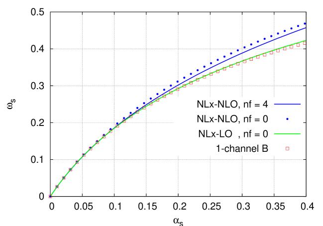
Figure 2: Hard Pomeron exponent $\omega_{\mathrm{s}}$ obtained in the NL$x$-NLO matrix formulation with $n_{f}=4$ (solid blue) and $n_{f}=0$ (dotted blue). The one-channel results [11] are also shown (red squares) and compared to those of the matrix model in NL$x$-LO approximation with $n_{f}=0$ (solid green). The calculation is done in the fixed coupling case.

We have numerically solved the implicit equations (5.9) in our matrix formulation in a range of $\alpha_{\mathrm{s}}$ up to 0.4, both at NL$x$-NLO and NL$x$-LO accuracy, for two values of $n_{f}=0$ and 4. The results for $\omega_{\mathrm{s}}$ versus $\alpha_{\mathrm{s}}$ are shown in fig. 2, where we compare with results obtained from our previous one-channel approach.

The NL$x$-LO curve at $n_{f}=0$ almost overlaps to the old one-channel result, thus showing the stability of the matrix formulation and the continuity with the one-channel approach. In fact, since at $n_{f}=0$ the kernel is diagonal, only the $gg$ entry determines $\omega_{\mathrm{s}}$. The small discrepancy is due to: (i) the momentum-conserving factor in front of $\tilde{\chi}_{1}$ in eq. (3.18) (it was a plain $1/\omega$ in the one-channel case); (ii) a non vanishing two-loop anomalous dimension (only for the low-energy part, actually) (we enforced vanishing anomalous dimension in the one-channel case). By including the NLO contributions we obtain a moderate increase of the Pomeron intercept, which slightly diminishes when quarks are also taken into account.

5.2 Effective characteristic function(s)

As already noted in the previous section, the contributions to the integral representation of the cross section stem from those values of $\omega$ and $\gamma$ such that

$$\det[1-\mathsf{K}(\alpha_{\mathrm{s}},\gamma,\omega)]=0\;.$$ (5.10)

which provides a relation between the moment index $\omega$ and the anomalous dimension variable $\gamma$. Solving eq. (5.10) for either $\omega$ or $\gamma$ defines the effective characteristic function and its dual effective anomalous dimension

$$\omega=\chi_{\mathrm{eff}}(\alpha_{\mathrm{s}},\gamma)\;,\qquad\gamma=\gamma_{\mathrm{eff}}(\alpha_{\mathrm{s}},\omega)\;.$$ (5.11)

While in the one-channel case we have only one perturbative branch of those functions, corresponding to the BFKL eigenvalue function $\chi_{+}(\gamma)$ and to the larger eigenvalue $\gamma_{+}(\omega)$ of the anomalous dimension matrix, in the matrix formulation we expect two branches. The second branch corresponds to the smaller eigenvalue $\gamma_{-}(\omega)$ which is dual to a second effective characteristic function $\chi_{-}(\gamma)$.

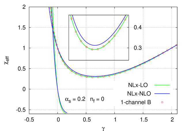
a)

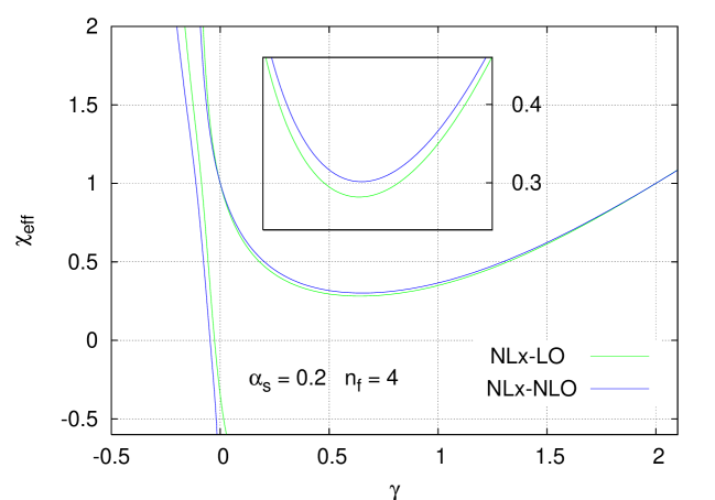
b)

Figure 3: Effective eigenvalue function obtained in the matrix formulation with full NL$x$-NLO accuracy (blue) and with NL$x$-LO accuracy (green) for $n_{f}=0$ (a) and $n_{f}=4$ (b). The steeply decreasing curves on the left side of each plot represent the minus-branches $\chi_{-}$, while the curves with a minimum around $\gamma\simeq 0.5$ represent the plus-branches $\chi_{+}$. The red circles reproduce the one-channel result in scheme B of ref. [11]. The calculation is done at fixed coupling $\alpha_{\mathrm{s}}=0.2$.

In fig. 3 we show the two branches of the effective characteristic functions obtained in the NL$x$-NLO and NL$x$-LO cases. We have considered here the asymmetric $\omega$-shift corresponding to the energy-scale $k^{2}$, with $\alpha_{\mathrm{s}}=0.2$. The $\chi_{+}$’s are characterised by the typical minimum around $\gamma\simeq 0.5$ whose value is nothing but $\omega_{\mathrm{s}}(\alpha_{\mathrm{s}})$. On the other hand, the $\chi_{-}$’s appear as steeply decreasing functions located around $\gamma\lesssim 0$ in the region shown in our plots.

The continuity of the resummation procedure when going from the one-channel to the two-channel formulation at $n_{f}=0$ is illustrated in fig. 3a by the overlapping of the ($+$)-branch of the NL$x$-LO curve to the circles corresponding to the one-channel scheme-B effective eigenvalue function. The NLO terms provide a slight increase of the ($+$)-branch in the region $0<\gamma<2$, and a small decrease of the ($-$)-branch at $\gamma<0$. At $n_{f}=0$ there is a crossing point of the two branches at negative $\gamma$ in either approximations.

The inclusion of quarks removes the crossing (with a mechanism similar to the degenerate level splitting in quantum mechanics) causing $\chi_{-}$ to be always on the left of $\chi_{+}$, as can be seen in fig. 3b. Quantitatively, the quark contribution lowers both $\chi_{+}$ in the region around the minimum (compare the two inserts in fig. 3) and $\chi_{-}$.

Note the two fixed points at $(\gamma,\omega=\chi_{\mathrm{eff}})$ = $(0,1)$ and $(2,1)$ of the ($+$)-branches. In the one-channel case these fixed points corresponds to momentum conservation in the collinear and anti-collinear limits respectively. In the two-channel formulation they imply that the anomalous dimension eigenvalue $\gamma_{+}(\omega=1)=0$; however, momentum sum rule is satisfied provided the corresponding left-eigenvector $\bar{v}_{+}=\begin{pmatrix}r&1\end{pmatrix}$ of the anomalous dimension matrix (cf. eq. (4.14)) be $\begin{pmatrix}1&1\end{pmatrix}$ at $\omega=1$, i.e., provided $r(\omega=1)=1$.

Actually, our matrix model presents a small violation of the momentum sum rule. In fact, by exploiting the fact that $\gamma_{+}(\omega=1)=0$ and by using eqs. (2.19) and (4.16) we have (at $\omega=1$)

$$\dot{q}+\dot{g}=\begin{pmatrix}1&1\end{pmatrix}\Gamma\begin{pmatrix}q\\ g\end{pmatrix}=\gamma_{-}\,\frac{1-r}{1+r\rho}(q-\rho g)\;.$$ (5.12)

The computation of the prefactor $\gamma_{-}\,(1-r)\rho/(1+r\rho)$ versus $\alpha_{\mathrm{s}}$ shown in tab. 1 gives us an estimate of the relative amount of momentum non-conservation; the violation is of order $\alpha_{\mathrm{s}}^{2}$ for the NL$x$-LO scheme, and of order $\alpha_{\mathrm{s}}^{3}$ for the scheme with NLO terms included.

$\alpha_{\mathrm{s}}$	NL$x$-LO	NL$x$-NLO	NL$x$-LO/$\alpha_{\mathrm{s}}^{2}$	NL$x$-NLO/$\alpha_{\mathrm{s}}^{3}$
0.025	0.00019	0.0000031	0.302	0.199
0.050	0.00072	0.0000208	0.287	0.167
0.100	0.00260	0.0001303	0.260	0.130
0.150	0.00534	0.0003437	0.237	0.102
0.200	0.00872	0.0006107	0.218	0.076

Table 1: Estimate of momentum sum rule violation. The quantity $\gamma_{-}\,(1-r)\rho/(1+r\rho)$ at $\omega=1$ has been computed for various values of $\alpha_{\mathrm{s}}$ (column 1) in the NL$x$-LO (column 2) and NL$x$-NLO (column 3) schemes. Column 4 (resp. 5) shows that the NL$x$-LO (NL$x$-NLO) violation is of order $\alpha_{\mathrm{s}}^{2}$ ($\alpha_{\mathrm{s}}^{3}$).

6 Numerical results with running coupling

In this section we shall present results obtained by solving eq. (2.1) in $(x,\boldsymbol{k})$-space, including a running coupling. The basic structure of the ensuing integral equation follows from eq. (3.27) and reads ($Y\equiv\log 1/x$)

$$\mathcal{G}_{ab}(Y;k,k_{0}) =\delta_{ab}\Theta(Y)\frac{\delta(k^{2}-k_{0}^{2})}{\pi}+\sum_{c}\int_{x}^{1}\frac{\mathrm{d}z}{z}\int\mathrm{d}k^{\prime}{}^{2}\Big{[}\hat{\alpha}(q^{2})\delta_{ag}\delta_{gc}K_{0}(z;k,k^{\prime})$$

$$\qquad+\hat{\alpha}(k_{>}^{2})\mathsf{K}_{\mathrm{coll},ac}(z;k,k^{\prime})+\hat{\alpha}^{2}(k_{>}^{2})\mathsf{K}_{1,ac}(z;k,k^{\prime})\Big{]}\mathcal{G}_{cb}\big{(}\log\frac{z}{x};k^{\prime},k_{0}\big{)}$$ (6.1)

(the explicit expressions of the kernels $K_{0}$, $\mathsf{K}_{\mathrm{coll}}$ and $\mathsf{K}_{1}$ in the equation above are given in app. C). We shall extract Green functions and splitting functions, using the methods described in [11, 12, 23]. In both the coupling and the kernels we use a fixed number of flavours, $n_{f}=4$. The coupling runs with a 2-loop $\beta$ function, and is normalised such that $\alpha_{\mathrm{s}}(3\,\text{GeV})=0.256$. The infrared region of the coupling is regularized by setting it to zero for scales $\mu<\mu_{0}=0.75\,\text{GeV}$.

The results that we shall show are those of the model described above (NL$x$-NLO), and also those for a model in which the higher twist part of $K_{0,qg}$ has been supplemented with (symmetric) $1/(1+\gamma)^{2}$ and $1/(2+\omega-\gamma)^{2}$ terms so that not only the $\alpha_{\mathrm{s}}^{2}/\omega$ but also $\alpha_{\mathrm{s}}^{3}/\omega^{2}$ terms of the $qq$, $qg$ and $gg$ splitting functions are in the $\overline{\mathrm{MS}}$ scheme. We shall denote this second model NL$x$-NLO⁺. We shall also compare to results obtained in our earlier single-channel work [12] (scheme B), where we used a 1-loop coupling, $n_{f}=0$ in the kernel (but $n_{f}=4$ in the coupling) and for which the NLO piece of the effective $P_{gg}$ splitting function was identically zero.

6.1 Green functions

The Green function for the matrix evolution is itself a matrix in flavour space. Physically the most interesting part is that involving gluonic sources, and this is shown in fig. 4.

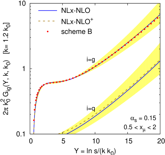
Figure 4: Gluon-induced part of the Green function for the NL$x$-NLO and NL$x$-NLO⁺ models, compared to the results of [12] (scheme B). For the models of this paper both $\mathcal{G}_{gg}$ and $\mathcal{G}_{qg}$ are shown. The value chosen for the coupling, $\alpha_{\mathrm{s}}=0.15$, corresponds to $k_{0}\simeq 20\,\text{GeV}$. The band indicates the spread in the result for the NL$x$-NLO model when varying the renormalisation scale in the range $0.5<x_{\mu}<2$.

The old and new resummations give nearly identical results for the $\mathcal{G}_{gg}$ part of the result, indicative of the stability of the resummation procedure. Furthermore, the differences between them are much smaller than renormalisation scale uncertainty, which grows with $Y$. The growth with $Y$ of the scale uncertainty can be understood as an indication of underlying scale dependence of the effective BFKL exponent.

The $\mathcal{G}_{qg}$ channel can be given only within the new resummations. As would be expected, the quark component is suppressed by a factor $\sim\alpha_{\mathrm{s}}$ compared to the gluon component. A consequence of the fact that the quarks are only generated radiatively is the scale dependence in their normalisation as well as in their growth with $Y$. We note that the change induced by the NNLO scheme-dependent higher-twist part of $K_{0,qg}$ (NL$x$-NLO⁺ versus NL$x$-NLO) is small, despite the fact that the region $k\sim k_{0}$ that we study is that most likely to be sensitive to this higher-twist contribution.

6.2 Splitting functions

The extraction of splitting functions is carried much in the same way as in the one-channel case described in [23, 11]. There a special (infrared) inhomogeneous term was included in the equation for the Green function such as to ensure that the resulting integrated gluon distribution satisfies $xg(x,\mu^{2})=1$, independently of $x$, for $\mu^{2}$ set equal to some given $Q^{2}$. With that inhomogeneous term fixed, the $xP_{gg}(x,Q^{2})$ splitting function was then obtained as $\frac{\partial}{\partial\ln x}\frac{\partial}{\partial\ln\mu^{2}}xg(x,\mu^{2})|_{\mu^{2}=Q^{2}}$. In the matrix case, we have a 2-component vector of inhomogeneous terms: we can choose it such that $xq(x,\mu^{2})=0$, $xg(x,\mu^{2})=1$ for $\mu^{2}=Q^{2}$, in which case we obtain

$$\left(\!\begin{array}[]{c}xP_{qg}\\ xP_{gg}\end{array}\!\right)=\frac{\partial}{\partial\ln x}\frac{\partial}{\partial\ln\mu^{2}}\left.\left(\!\begin{array}[]{c}xq(x,\mu^{2})\\ xg(x,\mu^{2})\end{array}\!\right)\right|_{\mu^{2}=Q^{2}}\,.$$ (6.2)

Alternatively we can set the inhomogeneous terms so as to ensure that $q(x,\mu^{2})=1$, $g(x,\mu^{2})=0$ for $\mu^{2}=Q^{2}$ and we then extract $P_{qq}$ and $P_{gq}$.

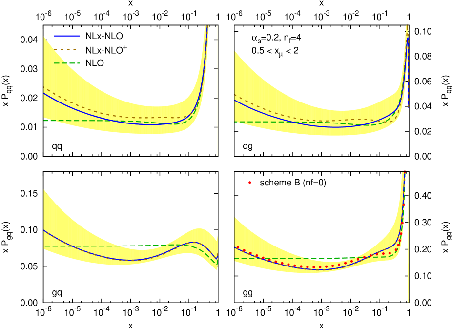
Figure 5: The matrix of NL$x$-NLO (and NL$x$-NLO⁺) splitting functions together with their scale uncertainty and the NLO splitting functions for comparison. In the $gg$ channel, we also show the old scheme B result ($n_{f}=0$, no NLO contributions, 1-loop coupling) of [11]. The band corresponds to the span of results (NL$x$-NLO) obtained if one chooses $x_{\mu}=0.5$ and $x_{\mu}=2.0$.

The matrix of effective splitting functions as determined with this method is shown in fig. 5, for both our kernels and with a scale $Q\simeq 6\,\text{GeV}$, giving $\alpha_{\mathrm{s}}(Q^{2})=0.2$. For reference we plot also the exact NLO splitting functions and our previous results for the single-channel evolution. Considering first the $gg$ channel, the results are rather similar to the old ones, and in particular maintain the characteristic dip [13] around $x=10^{-3}$ that has been seen also by the authors of [16]. This dip is present also in the $gq$ channel, and indeed the $gq$ channel is rather similar in a range of features to the $gg$ channel, which is natural since it is largely driven by the summation of the $g\to g$ branching. Among the common features is the slight but noticeable difference compared to the NLO splitting functions at moderate $x$ ($x\gtrsim 0.1$). The detailed origin of this characteristic is not really understood, but may well be connected with the fact that the various pieces of the NLO $gg$ splitting function are effectively placed in different parts of our evolution kernel, and then subjected to non-trivial (higher order) non-linear effects in their recombination into the final effective splitting function.

Concerning the scale dependence of the $P_{gj}$ channels, as for the Green function, it grows significantly towards small $x$, and again this is a sign of scale dependence of the small-$x$ intercept. One notes non-negligible scale dependence also at moderate $x$. Generally, down to moderately small $x$, the scale dependence of the NL$x$-NLO splitting functions (all channels) is rather similar to that (not shown) of the plain NLO splitting functions.

The two $P_{qj}$ channels differ fundamentally from the $P_{gj}$ channels in that they are non-zero at small $x$ starting only at NL$x$ and at NLO. Thus there is a sense in which our NL$x$-NLO treatment is effectively a leading order treatment for these channels, at least as concerns their normalisation (the small-$x$ growth is driven by iterations in the gluon channel, so one expects this to be under better control). This is visible in the much larger scale dependence for these channels. They also have some (modest) sensitivity to the difference between the NL$x$-NLO and NL$x$-NLO⁺ kernels, whereas in the $P_{gj}$ channels there was almost no sensitivity to this difference (even though the difference is NL$x$ in all channels). A general feature of the $P_{qj}$ splitting functions is that they are rather similar to the NLO splitting functions (more so than in the gluon channel). In particular, though like the $P_{gj}$ splitting functions they have a dip around $x=10^{-3}$, this dip is considerably shallower. The conclusion here is that the NLO $P_{qj}$ splitting functions can probably be considered a good approximation to the full splitting functions for $x$ as low as $10^{-4}$.

An important cross-check of the methods used to extract the splitting functions is that the results should be independent (modulo higher-twist contributions) of the infrared regularisation of the coupling, i.e. independent of the scale $\mu_{0}$ below which the coupling is set to zero. To this end we have extracted the splitting functions with $\mu_{0}$ increased from $0.75\,\text{GeV}$ to $1\,\text{GeV}$ (corresponding to reducing $\alpha_{\mathrm{s}}(\mu_{0})$ from $0.58$ to $0.45$) and find that the results change only by a few percent. As in previous work [23, 11] we find that these factorization violations scale roughly as $1/Q$ rather than as $1/Q^{2}$, a characteristic perhaps attributable to resummation effects, which could quite conceivably modify typical collinear $1/Q^{2}$ power-suppressed effects such that they become $1/Q^{2-2\gamma}$ with an effective $\gamma\simeq 1/2$.

		NL$x$-NLO				NL$x$-NLO+
$\alpha_{\mathrm{s}}$	$Q$ [GeV]	$\sum_{j}\Gamma_{jq}(1)$		$\sum_{j}\Gamma_{jg}(1)$		$\sum_{j}\Gamma_{jq}(1)$		$\sum_{j}\Gamma_{jg}(1)$
$0.20$	6	0.	0079	-0.	0059	0.	0074	-0.	0055
$0.15$	20	0.	0021	-0.	0015	0.	0018	-0.	0012
$0.10$	220	0.	00012	-0.	00003	0.	00006	0.	00002

Table 2: Momentum sum-rule violation in the NL$x$-NLO and NL$x$-NLO⁺ models for three values of $\alpha_{\mathrm{s}}$. The numerical uncertainty is roughly $\pm 1$ on the last digit of each result.

We close this section by showing in table 2 the degree of momentum sum-rule (MSR) violation in the splitting functions for three values of $\alpha_{\mathrm{s}}$. From just a small number of values it is difficult to establish the exact scaling law, and in particular it is difficult to determine the relative admixture of higher-twist and perturbative components in the MSR violations. Nevertheless, one sees that the MSR violation vanishes very rapidly as $\alpha_{\mathrm{s}}$ decrease, suggesting that a significant component of it is non-perturbative in origin. This conclusion is borne out by studies which show that the amount of MSR violation depends somewhat also on $\mu_{0}$, the infrared cutoff scale for the coupling.

7 Discussion

We have proposed here a matrix evolution equation for the flavour singlet, unintegrated quark and gluon densities, which generalizes the DGLAP and BFKL equations in the relevant limits.

The matrix approach (secs. 2 and 3) is supposed to unify collinear and high-energy factorizations in both partonic channels, and is not necessarily guaranteed to actually work, because of the various crossed consequences that the above factorizations have: consider, for instance, the anomalous dimension resummation formulae arising from $\boldsymbol{k}$-factorization [5, 8] and the $\gamma\leftrightarrow 1+\omega-\gamma$ symmetry of the BFKL kernel [9, 10] arising from collinear factorization. It is therefore a nontrivial result of this paper that our resummed splitting functions do satisfy collinear factorization in matrix form, as shown in secs. 4 and 6. In this respect, our approach defines, by the matrix evolution, some unintegrated densities that are appropriate both in the collinear and in the small-$x$ limits. It would be interesting to explore the relationship of such explicit construction with alternative studies [22, 24].

Furthermore, we want to incorporate exact low-order anomalous dimensions in our matrix kernel, say in the $\overline{\mathrm{MS}}$ scheme. We find, in this context, a new kind of consistency relations on the kernels, due to a possible clash of exact low-order expressions with a novel NL$x$ resummation formula for $\Gamma_{gq}$, arising in the matrix evolution (sec. 4). We prove such relations to be satisfied by our construction in the $\overline{\mathrm{MS}}$ scheme at NLO, but marginally violated by $n_{f}/N_{c}^{2}$-suppressed terms at NNLO. We are thus able to complete our construction with exact NLO anomalous dimensions and NL$x$ kernel, and we postpone the analysis of the NNLO accuracy, which is however nearly incorporated (in the NL$x$ approximation) in our NLO⁺ version.

The frozen-$\alpha_{\mathrm{s}}$ features of our matrix model are characterized by the previously mentioned resummation formulae of sec. 4, and by the hard Pomeron exponent and effective eigenvalue functions of sec. 5. One should notice the basic continuity of our matrix approach with the single-channel case in the $n_{f}=0$ limit, and the corresponding agreement of the leading effective eigenvalue function with the ABF approach. Additionally, we provide here the subleading effective eigenvalue at $n_{f}=4$, corresponding to the $\gamma_{-}$ eigenvalue of the anomalous dimension.

We are finally able to provide the whole matrix of resummed splitting functions in sec. 6. Roughly speaking, the outcome shows that resummation effects are small in the $P_{qa}$ entries up to $x$-values as small as $10^{-4}$, while the shallow dip is the main qualitative feature of both $P_{ga}$ entries, with resummation effects starting below $x\simeq 10^{-3}$.

We notice that the above results are in the $\overline{\mathrm{MS}}$ scheme up to NLO (including approximately NNLO in their NLO⁺ version), but generally differ from it at higher orders. However, resummation effects in the scheme change have been studied in [14] and turn out to be of the order of the scale uncertainty. For this reason we believe that the above results can be safely used in the study of structure functions and other cross-sections, by supplementing them with the corresponding coefficient functions or impact factors.

Appendix A Recursive expressions for the anomalous dimensions

In this appendix we show how eqs. (2.20) are obtained. Let us first rewrite eqs. (2.18,2.19) in $\gamma$-space, by noting that $\gamma=\partial_{\log Q^{2}}$:

$$\gamma\,f_{i}(\gamma,\omega)={\mathcal{F}}_{i}(\gamma,\omega)=\Gamma_{ij}(\omega)f_{j}(\gamma,\omega)+\text{h.t.}$$ (A.1)

where “h.t.” stands for higher-twist contributions characterised by being regular at $\gamma=0$. It follows that, in matrix notation,

$$\gamma^{2}f=\gamma(\Gamma f+\text{h.t.})=\Gamma(\gamma f)+\text{h.t.}=\Gamma^{2}f+\text{h.t.}$$ (A.2)

and, by induction,

$$\gamma^{n}f=\Gamma^{n}f+\text{h.t.}\;,$$ (A.3)

Secondly, we consider eq. (2.17) and expand the matrix kernel $\mathsf{K}$ in powers of gamma (according to the notations following eq. (2.11)), obtaining

$${\mathcal{F}}=\left(\sum_{m=0}\mathsf{K}^{(m)}\gamma^{m-1}\right){\mathcal{F}}+{\mathcal{F}}^{\mathrm{source}}=\sum_{m=0}\mathsf{K}^{(m)}\gamma^{m}f+{\mathcal{F}}^{\mathrm{source}}=\sum_{m=0}\mathsf{K}^{(m)}\Gamma^{m}f+\text{h.t.}\;,$$ (A.4)

By comparing eqs. (A.1) and (A.4) we derive the implicit equation

$$\Gamma=\sum_{m=0}\mathsf{K}^{(m)}\Gamma^{m}\;,$$ (A.5)

which allows us to determine the effective anomalous dimension matrix $\Gamma$ in terms of the matrix kernel $\mathsf{K}$.

It is now straightforward to compute the perturbative coefficients $\Gamma_{n}$ defined in eq. (2.12). By expanding eq. (A.5) to first order in $\hat{\alpha}$ yields ($m=0$)

$$\hat{\alpha}\Gamma_{0}=\hat{\alpha}\mathsf{K}_{0}^{(0)}$$ (A.6)

from which eq. (2.20a) follows. By expanding eq. (A.5) to second order in $\hat{\alpha}$ yields ($m\leq 1$)

$$\hat{\alpha}\Gamma_{0}+\hat{\alpha}^{2}\Gamma_{1}=\hat{\alpha}\mathsf{K}_{0}^{(0)}+\hat{\alpha}^{2}\mathsf{K}_{1}^{(0)}+\hat{\alpha}\mathsf{K}_{0}^{(1)}\hat{\alpha}\Gamma_{0}\;.$$ (A.7)

At frozen coupling, the operators $\mathsf{K}_{0}^{(1)}$ and $\hat{\alpha}$ commute. By then collecting the ${\cal O}\left(\hat{\alpha}^{2}\right)$ terms and remembering that $\Gamma_{0}=\mathsf{K}_{0}^{(0)}$ we get

$$\hat{\alpha}^{2}\Gamma_{1}=\hat{\alpha}^{2}(\mathsf{K}_{1}^{(0)}+\mathsf{K}_{0}^{(1)}\mathsf{K}_{0}^{(0)})$$ (A.8)

from which eq. (2.20b) follows. A similar iteration procedure produces eq. (2.20c) and higher orders.

In the running coupling case, we have an additional commutator term starting at second order, namely

$$\hat{\alpha}[\mathsf{K}_{0}^{(1)},\hat{\alpha}]\mathsf{K}_{0}^{(0)}\;.$$ (A.9)

By using the expansion

$$\hat{\alpha}=\hat{\alpha}_{\mu}-\beta_{0}\hat{\alpha}_{\mu}^{2}\log\textstyle{\frac{k^{2}}{\mu^{2}}}+{\cal O}\left(\hat{\alpha}_{\mu}^{3}\right)\;,$$ (A.10)

the commutator reads

$$[\mathsf{K}_{0}^{(1)},\hat{\alpha}]=-\beta_{0}\hat{\alpha}^{2}[\mathsf{K}_{0}^{(1)},\log\textstyle{\frac{k^{2}}{\mu^{2}}}]+{\cal O}\left(\hat{\alpha}^{3}\right)\;,$$ (A.11)

thus producing, by eq. (A.9), a contribution of order $\hat{\alpha}^{3}$ to the anomalous dimension matrix. Note however that the NL$x$ term of order $\alpha_{\mathrm{s}}^{3}/\omega^{2}$ vanishes, because the $gg$ entry of $\mathsf{K}_{0}^{(1)}$ has no leading $1/\omega$ term.

Extending the above procedure to higher orders, we see that at each order (say NⁿLO) the anomalous dimension gets a new term $\mathsf{K}_{n}^{(0)}$ but also a series of other terms which are combinations of the anomalous dimensions at the lower orders $<n$.

Appendix B Splitting functions and anomalous dimensions

Singlet anomalous dimensions and splitting functions at lowest order appear in many of our formulas. The former are given by ($T_{f}\equiv T_{r}n_{f}$)

$$P_{qq,0}(z) =C_{F}\left[\frac{2}{(1-z)_{+}}-1-z+\frac{3}{2}\delta(1-z)\right]$$ (B.1)

$$P_{qg,0}(z) =2T_{f}[z^{2}+(1-z)^{2}]$$ (B.2)

$$P_{gq,0}(z) =C_{F}\frac{1+(1-z)^{2}}{z}$$ (B.3)

$$P_{gg,0}(z) =2C_{A}\left[\frac{1}{z}+\frac{1}{(1-z)_{+}}-2+z-z^{2}\right]+\frac{11C_{A}-4T_{f}}{6}\delta(1-z)\;.$$ (B.4)

The anomalous dimensions, i.e., the Mellin transforms of the splitting functions, are given by

$$\Gamma_{qq,0}(\omega) =C_{F}\left[2\psi(1)-2\psi(\omega+1)-\frac{1}{\omega+1}-\frac{1}{\omega+2}+\frac{3}{2}\right]$$ (B.5)

$$\Gamma_{qg,0}(\omega) =2T_{f}\left(\frac{1}{\omega+1}-\frac{2}{\omega+2}+\frac{2}{\omega+3}\right)$$ (B.6)

$$\Gamma_{gq,0}(\omega) =C_{F}\left[\frac{2}{\omega}-\frac{2}{\omega+1}+\frac{1}{\omega+2}\right]$$ (B.7)

$$\Gamma_{gg,0}(\omega) =2C_{A}\left[\frac{1}{\omega}+\psi(1)-\psi(\omega+1)-\frac{2}{\omega+1}+\frac{1}{\omega+2}-\frac{1}{\omega+3}+\frac{11}{12}\right]-\frac{2T_{f}}{3}\;.$$ (B.8)

The gluon anomalous dimensions $\Gamma_{gq,0}$ and $\Gamma_{gg,0}$ are singular at $\omega=0$. The regular parts are defined by subtraction of the $\omega$-pole, namely

$$A_{gq}(\omega)\equiv\Gamma_{gq,0}(\omega)-\frac{2C_{F}}{\omega}\;,\qquad A_{gg}(\omega)\equiv\Gamma_{gg,0}(\omega)-\frac{2C_{A}}{\omega}\;.$$ (B.9)

Their values at $\omega=0$ are

$$\begin{pmatrix}\Gamma_{qq,0}(0)&\Gamma_{qg,0}(0)\\[8.61108pt] A_{gq}(0)&A_{gg}(0)\end{pmatrix}=\begin{pmatrix}0&\frac{4T_{f}}{3}\\[8.61108pt] -\frac{3C_{F}}{2}&-\frac{11C_{A}+4T_{f}}{6}\end{pmatrix}\;.$$ (B.10)

Appendix C Kernels and characteristic functions

Our method of resumming energy-scale dependent terms relies on the introduction of improved kernels whose characteristic functions $\chi_{\omega}(\gamma)$ are $\omega$-dependent. In general such characteristic functions are symmetric in the $\gamma\to 1+\omega-\gamma$ transformation and have the following structure:

$$\frac{1}{\omega}\chi_{\omega}(\gamma)=\mathcal{M}(\omega)\left[\chi_{L}(\gamma)+\chi_{L}(1+\omega-\gamma)\right]\;,$$ (C.1)

where the left-projection $\chi_{L}$ contains collinear (and possibly higher-twist) singularities only in the half-plane $\Re(\gamma)\leq 0$.

The $\omega$-dependence in the argument of the second $\chi_{L}$ term imposes kinematical constraints on the longitudinal momentum fraction variable $z$ conjugated to $\omega$. In fact, by denoting by $zM(z)$ and $K_{L}$ the inverse Mellin transforms of $\mathcal{M}$ and $\chi_{L}$ respectively, we have

$$K(z;\boldsymbol{k},\boldsymbol{k}^{\prime})\equiv\frac{1}{k^{2}}\int\frac{\mathrm{d}\omega}{2\pi\mathrm{i}}\;z^{-\omega}\int\frac{\mathrm{d}\gamma}{2\pi\mathrm{i}}\;\left(\frac{k^{2}}{k^{\prime}{}^{2}}\right)^{\gamma}\;\frac{1}{\omega}\chi_{\omega}(\gamma)=z^{\prime}M(z^{\prime})K_{L}(k_{>},k_{<})\;,$$ (C.2)

where $k_{<}\equiv\min(k,k^{\prime})$, $k_{>}\equiv\max(k,k^{\prime})$ and $z^{\prime}\equiv z\cdot\max(1,k^{\prime}{}^{2}/k^{2})$. Since $0<z^{\prime}<1$, the kinematical constraint $k^{\prime}{}^{2}<k^{2}/z$ follows.

The lowest-order matrix kernel $\mathsf{K}_{0}$ in $(z,\boldsymbol{k})$-space can be derived from eq. (3.2) and reads

$$[\hat{\alpha}\mathsf{K}_{0}](z;k,k^{\prime}) =\hat{\alpha}(q^{2})\begin{pmatrix}0&0\\[8.61108pt] 0&2C_{A}K_{0}(z;k,k^{\prime})\end{pmatrix}$$ (C.3)

$$+\hat{\alpha}(k_{>}^{2})\left[z^{\prime}\begin{pmatrix}P_{qq,0}(z^{\prime})&P_{qg,0}(z^{\prime})\\[8.61108pt] P_{gq,0}(z^{\prime})&P_{gg,0}(z^{\prime})-\frac{2C_{A}}{z^{\prime}}\end{pmatrix}K_{c}(k,k^{\prime})+z^{\prime}\begin{pmatrix}0&\Delta_{qg}(z^{\prime})K_{\mathrm{ht}}(k,k^{\prime})\\[8.61108pt] 0&0\end{pmatrix}\right]$$

having defined

$$K_{c}(k,k^{\prime}) \equiv\frac{1}{k_{>}^{2}}\,,$$ (C.4)

$$K_{\mathrm{ht}}(k,k^{\prime}) \equiv\frac{2}{3}\frac{k_{<}^{2}}{k_{>}^{4}}\,,$$ (C.5)

$$\Delta_{qg}(z) \equiv\delta_{qg}\,3(1-z)^{2}\;.$$ (C.6)

The terms in square brackets in eq. (C.3) correspond to the operator $\mathsf{K}_{\mathrm{coll}}$ introduced in eq. (6.1). The action of the first term $\sim\hat{\alpha}(q^{2})$ on a test function $f(x,k)$ is

$$\int_{x}^{1}\frac{\mathrm{d}z}{z}\int\mathrm{d}k^{\prime}{}^{2}\; \hat{\alpha}(q^{2})K_{0}(z;k,k^{\prime})f\big{(}\frac{x}{z},k^{\prime}\big{)}$$ (C.7)

$$\equiv\int_{x}^{1}\frac{\mathrm{d}z}{z}\int\frac{\mathrm{d}^{2}\boldsymbol{q}}{\pi q^{2}}\;\hat{\alpha}(q^{2})\left[f\big{(}\frac{x}{z},|\boldsymbol{k}+\boldsymbol{q}|\big{)}\Theta(k^{2}-zk^{\prime}{}^{2})-\Theta(k-q)f\big{(}\frac{x}{z},k\big{)}\right]\;,$$

while the action of the terms $\sim\hat{\alpha}(k_{>}^{2})$, e.g. the higher-twist one, is

$$\int_{x}^{1} \frac{\mathrm{d}z}{z}\int\mathrm{d}k^{\prime}{}^{2}\;\hat{\alpha}(k_{>}^{2})z^{\prime}\Delta_{qg}(z^{\prime})K_{\mathrm{ht}}(k,k^{\prime})f\big{(}\frac{x}{z},k^{\prime}\big{)}$$ (C.8)

$$\equiv \int_{x}^{1}\frac{\mathrm{d}z}{z}\bigg{\{}\int_{0}^{k^{2}}\mathrm{d}k^{\prime}{}^{2}\;\hat{\alpha}(k^{2})z\Delta_{qg}(z)+\int_{k^{2}}^{k^{2}/z}\mathrm{d}k^{\prime}{}^{2}\;\hat{\alpha}(k^{\prime}{}^{2})z\frac{k^{\prime}{}^{2}}{k^{2}}\Delta_{qg}\big{(}z\frac{k^{\prime}{}^{2}}{k^{2}}\big{)}\bigg{\}}K_{\mathrm{ht}}(k,k^{\prime})f\big{(}\frac{x}{z},k^{\prime})\;.$$

In order to obtain $\mathsf{K}_{1}(z;k,k^{\prime})$ according to eq. (3.22), we start by computing the first term proportional to $\chi_{c}\to K_{c}$. The inverse Mellin transform of $\Gamma_{1}^{(\overline{\mathrm{MS}})}$ is just the matrix of the two-loop singlet splitting functions in the $\overline{\mathrm{MS}}$-scheme [27]. The inverse Mellin tranform of the subtraction $\mathsf{K}_{0}^{(1)}\mathsf{K}_{0}^{(0)}$ can be either computed by inverting the expressions listed in eq. (3.34), or by convolution in $z$-space of the corresponding factors. Here we choose the second method, by computing first the analytic expressions of all factors in eq. (3.34) and then the numerical convolution of the ensuing functions. We already obtained the Mellin transform of $\Delta_{qg}$ in eq. (C.6); the transforms of the $\Gamma_{ij}$ factors are just the one-loop splitting functions reported in eqs. (B.5-B.8); the remaining functions are listed below:

$$\int\frac{\mathrm{d}\omega}{2\pi\mathrm{i}}\;z^{-\omega}\;c_{c}(\omega)=z\,,$$ (C.9)

$$\int\frac{\mathrm{d}\omega}{2\pi\mathrm{i}}\;z^{-\omega}\;\frac{2C_{A}}{\omega}c_{0}(\omega)=2C_{A}\log(1-z)\,,$$ (C.10)

$$\int\frac{\mathrm{d}\omega}{2\pi\mathrm{i}}\;z^{-\omega}\;\chi_{\mathrm{ht}}(0,\omega)=\frac{2}{3}\left[\delta(1-z)+z^{2}\right]\,.$$ (C.11)

Finally, we need the inverse Mellin transform

$$\int\frac{\mathrm{d}\omega}{2\pi\mathrm{i}}\;z^{-\omega}\;\left(\frac{1}{\omega}-\frac{2}{1+\omega}\right)=1-2z\,,$$ (C.12)

and the kernel

$$K_{1,\mathrm{reg}}\equiv\tilde{K}_{1}-\tilde{\chi}_{1}^{(0)}K_{c},$$ (C.13)

whose $\omega$-shifted form occurs directly in eq. (3.27), and has characteristic function

$$\chi_{1,\mathrm{reg}} \equiv\tilde{\chi}_{1}-\tilde{\chi}_{1}^{(0)}\chi_{c}$$ (C.14)

$$=\chi_{1}-\chi_{1}^{\mathrm{run}}-\chi_{0}\left(\dot{\chi}_{0}+\chi_{c}\frac{A_{gg}(0)}{2C_{A}}\right)-\frac{C_{F}}{C_{A}}\chi_{c}\left(\chi_{c}\frac{\Gamma_{qg,0}(0)}{2C_{A}}+\chi_{\mathrm{ht}}\frac{\delta_{qg}}{2C_{A}}\right)-\tilde{\chi}_{1}^{(0)}\chi_{c}\;.$$

The numerical coefficients $A_{gg}(0),\Gamma_{qg,0}(0)$ can be found in eq. (B.10), $\delta_{qg}\equiv\Delta_{qg}(0)$ in eq. (3.8) and $\tilde{\chi}_{1}^{(0)}$ in eq. (3.33). Furthermore, the computation of the kernel $K_{1,\mathrm{reg}}$ requires the subtraction from the NL$x$ BFKL kernel [6, 7] of the running coupling terms and of additional kernels corresponding to the characteristic functions on the r.h.s. of eq. (C.14). They are given by

$$\chi_{c} \to\frac{1}{k_{>}^{2}}\,,$$ (C.15)

$$\chi_{0}\dot{\chi}_{0} \to-\frac{1}{4|k^{2}-k^{\prime}{}^{2}|}\left[\log^{2}\frac{k^{\prime}{}^{2}}{k^{2}}+4{\mathrm{Li}_{2}}\Big{(}1-\frac{k_{<}^{2}}{k_{>}^{2}}\Big{)}\right]\,,$$ (C.16)

$$\chi_{0}\chi_{c} \to\frac{1}{k_{>}^{2}}\log\Big{(}\frac{k_{>}^{2}}{k_{<}^{2}}-1\Big{)}-\frac{1}{k_{<}^{2}}\log\Big{(}1-\frac{k_{<}^{2}}{k_{>}^{2}}\Big{)}\,,$$ (C.17)

$$\chi_{c}^{2} \to\frac{1}{k_{>}^{2}}\left(\log\frac{k_{>}^{2}}{k_{<}^{2}}+2\right)\,,$$ (C.18)

$$\chi_{c}\chi_{\mathrm{ht}} \to\frac{1}{k_{>}^{2}}\left(1-\frac{1}{3}\frac{k_{<}^{2}}{k_{>}^{2}}\right)\,.$$ (C.19)

The resulting expression for $K_{1,\mathrm{reg}}$ is

$$K_{1,\mathrm{reg}}(k,k^{\prime}) =\frac{1}{4}\left\{\left(\frac{67}{9}-\frac{\pi^{2}}{3}-\frac{20T_{r}n_{f}}{9C_{A}}\right)\langle K_{0}\rangle(k,k^{\prime})+\frac{1}{{k^{\prime}}^{2}+k^{2}}\left[\frac{\pi^{2}}{3}+4{\mathrm{Li}_{2}}\big{(}\frac{k_{<}^{2}}{k_{>}^{2}}\big{)}\right]+\right.$$

$$-\frac{1}{32}\left(1+\frac{2T_{r}n_{f}}{C_{A}^{3}}\right)\left[\frac{2}{{k^{\prime}}^{2}}+\frac{2}{k^{2}}+\left(\frac{1}{{k^{\prime}}^{2}}-\frac{1}{k^{2}}\right)\log\left(\frac{k^{2}}{{k^{\prime}}^{2}}\right)\right]+$$

$$\left.-\left[3+\left(\frac{3}{4}-\frac{({k^{\prime}}^{2}+k^{2})^{2}}{32{k^{\prime}}^{2}k^{2}}\right)\right]\left(1+\frac{2T_{r}n_{f}}{C_{A}^{3}}\right)\int_{0}^{\infty}\frac{\mathrm{d}y}{k^{2}+y^{2}{k^{\prime}}^{2}}\;\log\left|\frac{1+y}{1-y}\right|\right\}+$$

$$+\frac{3}{2}\zeta(3)\delta(k^{2}-k^{\prime 2})+\frac{4{\mathrm{Li}_{2}}(1-k_{<}^{2}/k_{>}^{2})}{|{k^{\prime}}^{2}-k^{2}|}+$$

$$-4\frac{A_{gg}(0)}{2C_{A}}{\rm sgn}({k}^{2}-{k^{\prime}}^{2})\left(\frac{1}{k^{2}}\log\frac{|{k^{\prime}}^{2}-k^{2}|}{{k^{\prime}}^{2}}-\frac{1}{{k^{\prime}}^{2}}\log\frac{|{k^{\prime}}^{2}-k^{2}|}{{k}^{2}}\right)+$$

$$-\frac{C_{F}}{C_{A}}\frac{1}{k_{>}^{2}}\left[\frac{\Gamma_{qg,0}(0)}{2C_{A}}\left(\log\frac{k_{>}^{2}}{k_{<}^{2}}+2\right)+\frac{\delta_{qg}}{2C_{A}}\left(1-\frac{1}{3}\frac{k_{<}^{2}}{k_{>}^{2}}\right)\right]-\tilde{\chi}_{1}^{(0)}\frac{1}{k_{>}^{2}}\;.$$ (C.20)

where $\langle K_{0}\rangle$ denotes the azimuthal average of the LL$x$ BFKL kernel whose action on a test function $f(k)$ is given by

$$[\langle K_{0}\rangle f](k)=\int\mathrm{d}k^{\prime}{}^{2}\;\frac{1}{|{k^{\prime}}^{2}-k^{2}|}\left[f(k^{\prime})-\frac{2k_{<}^{2}}{k^{\prime}{}^{2}+k^{2}}f(k)\right]\;.$$ (C.21)

Finally, we provide the eigenvalue function of $K_{1,\mathrm{reg}}$ with kinematical constraints, which is given by $\chi_{1,\mathrm{reg}}{}_{,L}(\gamma)+\chi_{1,\mathrm{reg}}{}_{,L}(1+\omega-\gamma)$, and occurs directly in eq. (3.27). The left projection $\chi_{1,\mathrm{reg}}{}_{,L}$ of the eigenvalue function (C.14) can be computed starting from the expression of $\tilde{\chi}_{1L}$ in eq. (A.13) of ref. [11] and noticing that:
(i) here we have more terms to subtract, namely those proportional to $C_{F}/C_{A}$ and $\tilde{\chi}_{1}^{(0)}$;
(ii) in ref. [11] we subtracted the $n_{f}$-part of the double pole by letting $A_{gg}(0)\to 2C_{A}A_{1}(0)\equiv A_{gg}(0)+(C_{F}/C_{A})\Gamma_{qg,0}(0)$, while here we keep only $A_{gg}(0)$ in front of $\chi_{0}\chi_{c}$ since the $n_{f}$-dependent double pole is subtracted by the $\Gamma_{qg}\chi_{c}^{2}$ term.

Therefore, in order to complete the calculation we need the left projections of the following kernels:

$$[\chi_{c}^{2}]_{L}(\gamma) =[\chi_{cL}(\gamma)]^{2}+2\chi_{cL}(\gamma)=\frac{1}{\gamma^{2}}+\frac{2}{\gamma}\,,$$ (C.22)

$$[\chi_{c}\chi_{\mathrm{ht}}]_{L}(\gamma) =\chi_{cL}(\gamma)-\frac{1}{2}\chi_{\mathrm{ht}}{}_{L}(\gamma)=\frac{1}{\gamma}-\frac{1}{3(1+\gamma)}\;.$$ (C.23)

The final result is

$$\chi_{1,\mathrm{reg}}{}_{,L}(\gamma) =[\psi(1)-\psi(\gamma)]\left[\psi^{\prime}(\gamma)-\frac{A_{gg}(0)}{2C_{A}}\chi_{c}(\gamma)+\frac{67}{36}-\frac{\pi^{2}}{12}-\frac{5}{18}\frac{n_{f}}{C_{A}}\right]$$

$$\quad+\frac{1}{2}\psi^{\prime\prime}(\gamma)+\Pi(\gamma)-\Phi_{L}(\gamma)+\frac{\pi^{2}}{8}\left[\psi\Big{(}\frac{1+\gamma}{2}\Big{)}-\psi\Big{(}\frac{\gamma}{2}\Big{)}\right]+\frac{3}{4}\zeta(3)$$

$$\quad+\frac{1}{32}\left\{-3M(\gamma)+\left(1+\frac{n_{f}}{C_{A}^{3}}\right)\left[\frac{1}{4}\left(\frac{1}{\gamma^{2}}-\frac{1}{(1-\gamma)^{2}}\right)-\frac{1}{2}\left(\frac{1}{\gamma}-\frac{1}{1-\gamma}\right)\right.\right.$$

$$\qquad\qquad\qquad\qquad\qquad\qquad\qquad\;\left.\left.+\frac{1}{32}\Big{(}M(\gamma+1)+M(\gamma-1)\Big{)}-\frac{11}{16}M(\gamma)\right]\right\}$$

$$\quad-\frac{C_{F}}{2C_{A}^{2}}\left[\Gamma_{qg,0}(0)\left(\frac{1}{\gamma^{2}}+\frac{2}{\gamma}\right)+\delta_{qg}\left(\frac{1}{\gamma}-\frac{1}{3(1+\gamma)}\right)\right]-\frac{\tilde{\chi}_{1}^{(0)}}{\gamma}\;,$$ (C.24)

where

$$\Pi(\gamma) \equiv\int_{0}^{1}dt\;t^{\gamma-1}\frac{{\mathrm{Li}_{2}}(1)-{\mathrm{Li}_{2}}(t)}{1-t}=\sum_{n=0}^{\infty}\frac{\psi^{\prime}(n+1)}{n+\gamma}\,,$$ (C.25)

$$\Phi_{L}(\gamma) \equiv\sum_{n=0}^{\infty}(-1)^{n}\frac{\psi(n+1+\gamma)-\psi(1)}{(n+\gamma)^{2}}\,,$$ (C.26)

$$M(\gamma) \equiv\frac{1}{\gamma-{\textstyle\frac{1}{2}}}\left[\psi^{\prime}\Big{(}\frac{1+\gamma}{2}\Big{)}-\psi^{\prime}\Big{(}\frac{\gamma}{2}\Big{)}+\psi^{\prime}\Big{(}\frac{1}{4}\Big{)}-\psi^{\prime}\Big{(}\frac{3}{4}\Big{)}\right]\;.$$ (C.27)

The explicit form of $K_{1,\mathrm{reg}}$ in ($\boldsymbol{k},z$) space is obtained by use of eq. (C.2), or by introducing the kinematical constraints on eq. (C.20) directly. The final form of $\mathsf{K}_{1}(z;\boldsymbol{k},\boldsymbol{k}^{\prime})$ follows from eq. (3.27).

References

-
[1]
V.N. Gribov and L.N. Lipatov, Sov. J. Nucl. Phys. 15 (1972) 438;
G. Altarelli and G. Parisi, Nucl. Phys. B 126 (1977) 298;
Yu.L. Dokshitzer, Sov. Phys. JETP 46 (1977) 641. -
[2]
L.N. Lipatov, Sov. J. Nucl. Phys. 23 (1976) 338;
E.A. Kuraev, L.N. Lipatov and V.S. Fadin, Sov. Phys. JETP 45 (1977) 199;
I.I. Balitsky and L.N. Lipatov, Sov. J. Nucl. Phys. 28 (1978) 822;
L.N. Lipatov, Sov. Phys. JETP 63 (1986) 904. - [3] For a review of some research lines see, e. g., Small- Collaboration (Jeppe R. Andersen et al.), Eur. Phys. J. C48 (2006) 53.
-
[4]
V. S. Fadin and L. N. Lipatov,
JETP Lett. 49 (1989) 352
[Yad. Fiz. 50 (1989 SJNCA,50,712.1989) 1141];
Nucl. Phys. B 406 (1993) 259;
Nucl. Phys. B 477 (1996) 767.
V. S. Fadin, R. Fiore and A. Quartarolo, Phys. Rev. D 50 (1994) 2265; Phys. Rev. D 50 (1994) 5893.
V. S. Fadin, R. Fiore and M. I. Kotsky, Phys. Lett. B 359 (1995) 181; Phys. Lett. B 387 (1996) 593; Phys. Lett. B 389 (1996) 737.
V. S. Fadin, M. I. Kotsky and L. N. Lipatov, BUDKER-INP-1996-92, arXiv:hep-ph/9704267.
V. Del Duca, Phys. Rev. D 54 (1996) 989; Phys. Rev. D 54 (1996) 4474.
V.S. Fadin, R. Fiore, A. Flachi and M.I. Kotsky, Phys. Lett. B 422 (1998) 287. -
[5]
S. Catani, M. Ciafaloni and F. Hautmann,
Phys. Lett. B 242 (1990) 97;
Nucl. Phys. B 366 (1991) 135.
G. Camici and M. Ciafaloni, Phys. Lett. B 386 (1996) 341; Nucl. Phys. B 496 (1997) 305 [Erratum-ibid. B 607 (2001) 431]. - [6] V. S. Fadin and L. N. Lipatov, Phys. Lett. B 429 (1998) 127.
- [7] G. Camici and M. Ciafaloni, Phys. Lett. B 412 (1997) 396 [Erratum-ibid. B 417 (1998) 390]; Phys. Lett. B 430 (1998) 349.
- [8] S. Catani and F. Hautmann, Nucl. Phys. B 427 (1994) 475.
- [9] G. P. Salam, JHEP 9807 (1998) 019.
- [10] M. Ciafaloni and D. Colferai, Phys. Lett. B 452 (1999) 372. M. Ciafaloni, D. Colferai and G. P. Salam, Phys. Rev. D 60 (1999) 114036.
- [11] M. Ciafaloni, D. Colferai, G. P. Salam and A. M. Staśto, Phys. Rev. D 68 (2003) 114003.
- [12] M. Ciafaloni, D. Colferai, G. P. Salam and A. M. Staśto, Phys. Lett. B 576, (2003) 143.
- [13] M. Ciafaloni, D. Colferai, G. P. Salam and A. M. Staśto, Phys. Lett. B 587, (2004) 87.
- [14] M. Ciafaloni and D. Colferai, JHEP 0509 (2005) 069. M. Ciafaloni, D. Colferai, G. P. Salam and A. M. Staśto, Phys. Lett. B 635 (2006) 320.
- [15] G. Altarelli, R. D. Ball and S. Forte, Nucl. Phys. B 575, (2000) 313; G. Altarelli, R. D. Ball and S. Forte, Nucl. Phys. B 599, (2001) 383.
-
[16]
G. Altarelli, R. D. Ball and S. Forte,
Nucl. Phys. B 621, (2002) 359;
G. Altarelli, R. D. Ball and S. Forte, Nucl. Phys. B 674, (2003) 459;
G. Altarelli, R. D. Ball and S. Forte, Nucl. Phys. B 742, (2006) 1. - [17] R.S. Thorne, Phys. Rev. D 64 (2001) 074005; Phys. Lett. B 474 (2000) 372.
- [18] S. Alekhin et al., “HERA and the LHC - A workshop on the implications of HERA for LHC physics: Proceedings Part A,” arXiv:hep-ph/0601012.
- [19] C. D. White and R. S. Thorne, Phys. Rev. D 75, (2007) 034005.
- [20] B. Andersson, G. Gustafson, H. Kharraziha and J. Samuelsson, Z. Phys. C 71 (1996) 613.
- [21] J. Kwieciński, A. D. Martin and P. J. Sutton, Z. Phys. C 71 (1996) 585.
- [22] M. Ciafaloni, Nucl. Phys. B 296 (1988) 49.
- [23] M. Ciafaloni, D. Colferai and G. P. Salam, JHEP 0007 (2000) 054.
- [24] J.C. Collins, T. Rogers and A.M. Staśto (private communication).
- [25] M. Ciafaloni, Phys. Lett. B 429 (1998) 363; M. Ciafaloni and D. Colferai, Nucl. Phys. B 538 (1999) 187.
- [26] A. Vogt, S. Moch and J. A. M. Vermaseren, Nucl. Phys. B 691 (2004) 129.
- [27] G. Curci, W. Furmanski and R. Petronzio, Nucl. Phys. B 175, (1980) 27; W. Furmanski and R. Petronzio, Phys. Lett. B 97, (1980) 437.