Excitations and superfluidity in non-equilibrium Bose-Einstein condensates of exciton-polaritons

Abstract

We present a generic model for the description of non-equilibrium Bose-Einstein condensates, suited for the modelling of non-resonantly pumped polariton condensates in a semiconductor microcavity. The excitation spectrum and scattering of the non-equilibrium condensate with a defect are discussed.

1 Model and elementary excitation spectrum

Due to the finite polariton life time, the nature of polariton condensates [1] is fundamentally different from their superfluid ⁴He and atomic Bose-Einstein condensate counterparts: the polariton condensate has to be constantly replenished and arises as a dynamical equilibrium between pumping and decay. The theoretical modelling of such systems in which interactions, coherence, pumping and decay are equally important poses a challenge that was taken up only recently [2, 3, 4]. We will present here our mean field model of such condensates [4] and use it to study the excitation spectrum of a homogeneous non-equilibrium condensate and the problem of a small defect moving through it.

Our model does not include any details on the specific relaxation mechanisms of high-energy polaritons into the condensate, but is only based on some general assumptions: i) a single state of lower polaritons is macroscopically occupied so that it can be described by a classical field; ii) The momentum space can be devided in two parts: one part at small momenta where the coherence is important and one part at large momenta, where it is negligble. The polaritons in the high-momentum states act as a reservoir that replenishes the condensate. Under typical excitation conditions, the wave vector scale to separate both systems should be chosen of the order of a few $\mu\rm m^{-1}$; iii) The state of the reservoir is fully determined by its spatial polariton density $n_{R}(x)$. This last asumption requires that the reservoir polariton momentum distribution reaches some stationary state in momentum space. Under these assumptions, the condensate dynamics is to a first approximation described by a generalized Gross-Pitaevskii equation including loss and amplification terms

$$i\frac{\partial\psi}{\partial t}=\left\{-\frac{\hbar\nabla^{2}}{2m}+\frac{i}{2}\big{[}R(n_{R})-\gamma\big{]}+g\,|\psi|^{2}+2\tilde{g}\,n_{R}\right\}\psi,$$ (1)

where $m$ is the lower polariton mass, $\gamma$ its decay rate and $g$ is the strength of the polariton-polariton interaction within the condensate. The stimulated scattering of reservoir polaritons into the condensate is modeled by the term $R(n_{R})$ and the mean field interaction experienced by the condensate polaritons due to elastic collisions with the reservoir polaritons is given by $2\tilde{g}n_{R}$. The description (1) of the polariton condensate in terms of a deterministic classical field requires its density and phase fluctuations to be small. This regime is reached for pump powers well above the condensation threshold. The equation for the condensate dynamics is coupled to a diffusion equation for the reservoir polaritons

$$\frac{\partial n_{R}}{\partial t}=P-\gamma_{R}\,n_{R}-R\left(n_{R}\right)\left|\psi\left(x\right)\right|^{2}+D\nabla^{2}n_{R},$$ (2)

where $P$ is the pump rate due to external laser, $\gamma_{R}$ is the reservoir damping rate and $D$ its diffusion constant.

The stationary state and the elementary excitation spectrum of Eqns. (1) and (2) are discussed in Ref. [4]. In case the reservoir damping rate $\gamma_{R}$ is much larger than the condensate polariton damping rate $\gamma$, the condensate excitation spectrum is of the form

$$\omega_{\pm}(k)=-\frac{i\Gamma}{2}\pm\sqrt{\omega_{Bog}(k)^{2}-\frac{\Gamma^{2}}{4}},$$ (3)

Here, $\omega_{Bog}=[(k^{2}/2m+2\mu)(k^{2}/2m)]^{1/2}$ is the usual Bogoliubov dispersion of dilute Bose gases at equilibrium. The non-equilibrium nature of the system is quantified by the effective relaxation rate $\Gamma=\zeta\gamma$, where $\zeta$ depends on the pumping rate and on the functional form of $R(n_{R})$[4]. The most important differences with the excitation spectrum of equilibrium condensates is the non vanishing imaginary part of $\omega(k)$ for all $k\neq 0$ and the flatness of its real part for small $k$. The ‘+’-branch is diffusive for small wave vectors. A similar excitation spectrum was found in Ref. [2] for a specific model of nonequilibrium condensation, within a completely different approach, indicating that the form (3) is a general result for nonequilibrium condensates.

Our model is also straightforwardly applied to the Josephson oscillations between two condensates connected by quantum mechanical tunneling. The frequency of the density oscillations between the two wells is given by Eq.(3) with $\omega_{Bog}$ replaced by the equilibrium Josephson frequency [8].

2 Flow past a defect

One of the benchmark properties of condensed Bose systems is superfluidity. As a first step in the study of superfluidity in non-equilibrium systems, we will discuss the scattering of a moving condensate on a defect [5]. Experimentally, the condensate could be accelerated by applying an external force to it, e.g. by making a sample with a steep wedge in the cavity thickness or using surface acoustic waves to accelerate the polaritons [7]. Defects are naturally present in the form of disorder, but can also be deliberately created by structuring the cavity mirrors [6].

The perturbation on top of a condensate moving with velocity ${\mathbf{v}}$ due to a small defect potential $V_{def}=g\delta({\bf r})$ at rest can be studied in perturbation theory [5]. The change in condensate wave function is in momentum space given by

$$[\delta\psi({\mathbf{k}}),\delta\psi^{*}(2{\mathbf{k}}_{0}-{\mathbf{k}}),\delta n_{r}]^{T}=-\mathcal{L}_{\mathbf{v}}({\mathbf{k}})^{-1}[g\psi_{0}(0),\;-g\psi_{0}^{*}(0),\;0]^{T},$$ (4)

where $\mathcal{L}_{\mathbf{v}}({\mathbf{k}})$ the matrix from linearized motion equations (1),(2) around a steady state $n_{R}({\mathbf{x}})=n_{0}$, $\psi({\mathbf{x}})=\psi_{0}e^{i{\mathbf{k}}_{0}\cdot{\mathbf{x}}}$, where ${\mathbf{k}}_{0}=m{\mathbf{v}}$. Much about the response of the flowing condensate is learned by studying the poles ${\mathbf{k}}_{res}$ of $L_{\mathbf{v}}({\mathbf{k}})^{-1}$ in the complex ${\mathbf{k}}$-plane, i.e.

$$\omega_{{\mathbf{v}}\pm}({\mathbf{k}}_{res})=\omega_{\pm}({\mathbf{k}}_{res}-{\mathbf{k}}_{0})-{\mathbf{v}}\cdot({\mathbf{k}}_{res}-{\mathbf{k}}_{0})=0,$$ (5)

We restrict now our attention to the perturbation of the wave function in the direction of the defect velocity. The main contribution comes from the Fourier component with ${\mathbf{k}}\parallel{\mathbf{v}}$. The modulus of the resonant spatial frequency $k_{\parallel res}$ is plotted in Fig.1. The panels show from left to right an equilibrium condensate ($\Gamma=0$), a slightly non-equilibrium condensate ($\Gamma/\mu=0.01$) and a condensate where interaction effects and losses are comparable ($\Gamma=\mu/2$). Unlike for the temporal frequencies from Eq. (3), the imaginary part of the spatial frequencies should not be negative, but the spatial frequencies with a negative (positive) imaginary part correspond to positions on the left (right) hand side of the defect.

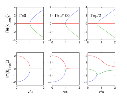
Figure 1: The real (upper panels) and corresponding imaginary (lower panels) part of the spatial frequencies (in units of the inverse of the healing length $\xi=\sqrt{\hbar/m\mu}$) that are excited by a stationary defect in a condensate moving at a speed $v$ for several values of $\Gamma/\mu$.

Let us start discussing the resonant spatial frequencies of the equilibrium condensate. The phase fluctuations, that give a pole at zero spatial frequency, do not couple to the external potential. The two other branches of $k_{\parallel res}$ are purely imaginary for velocities smaller than the speed of sound, implying that the condensate perturbation is spatially damped. The excitations are only virtually excited by the defect and no condensate momentum is dissipated. At $v=c$, there is a bifurcation, where a pair of conjugate imaginary roots turn real, the excitations go ‘on shell’, are radiated and dissipate the condensate momentum.

In the case of non-equilibrium condensates (central and right panels of Fig. 1), the bifurcation point is shifted to velocities $v<c$ and $\textrm{Im}(k_{\parallel,res})<0$. No spatial frequencies with zero imaginary part appear anymore. Therefore, in contrast to the equilibrium condensates, no sharp transition in the condensate perturbation as a function of its velocicy is expected.

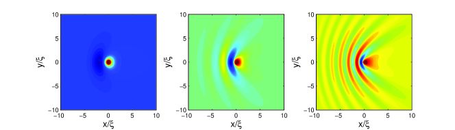
Figure 2: The perturbation of the condensate moving condensate due to a small defect at $x=0$. Condensate velocities: $v/c=0.7$ (left panel), $v/c=1.3$ (center panel) and $v/c=2$ (right panel). Effective damping rate $\Gamma=\mu/2$.

This is confirmed by the condensate perturbation in real space, shown in Fig. 2 for several velocities $v$. The condensate perturbation depends sensitively on the velocity $v$, but no sharp transition occurs. It is smoothened due to the finite polariton life time.

References

- [1] M. Richard et al., Phys. Rev. Lett. 94, 187401 (2005); J. Kasprzak et al., Nature 443, 409 (2006); H. Deng et al., Phys. Rev. Lett. 97, 14602 (2006); S. Christopoulos et al., Phys. Rev. Lett. 98, 126405 (2007).
- [2] M. H. Szymańska, J. Keeling, and P. B. Littlewood, Phys. Rev. Lett. 96, 230602 (2006).
- [3] D. Sarchi and V. Savona, condmat/0703106.
- [4] M. Wouters and I. Carusotto, condmat/0702431.
- [5] I. Carusotto and C. Ciuti, Phys. Rev. Lett. 93, 166401 (2004); I. Carusotto et al., ibid. 97, 260403 (2006).
- [6] O. El. Daïf et al., Appl. Phys. Lett. 88, 061105 (2006).
- [7] M.M. de Lima et al., Phys. Rev. Lett. 97, 045501 (2006).
- [8] G.J. Milburn et al., Phys. Rev. A 55, 4318 (1997).