Poisson-Vlasov : Stochastic representation and numerical codes

Abstract

A stochastic representation for the solutions of the Poisson-Vlasov equation, with several charged species, is obtained. The representation involves both an exponential and a branching process and it provides an intuitive characterization of the nature of the solutions and its fluctuations. Here, the stochastic representation is also proposed as a tool for the numerical evaluation of the solutions

1 Introduction

It is well known that the solutions of linear elliptic and parabolic equations, both with Cauchy and Dirichlet boundary conditions, have a probabilistic interpretation. This is a very classical field which may be traced back to the work of Courant, Friedrichs and Lewy [1] in the 20’s. In spite of the pioneering work of McKean [2], the question of whether useful probabilistic representations could also be found for a large class of nonlinear equations remained an essentially open problem for many years. It was only in the 90’s that, with the work of Dynkin[3] [4], such a theory started to take shape. For nonlinear diffusion processes, the branching exit Markov systems, that is, processes that involve both diffusion and branching, seem to play the same role as Brownian motion in the linear equations. However the theory is still limited to some classes of nonlinearities and there is much room for further mathematical improvement.

Another field, where considerable recent advances were achieved, was the probabilistic representation of the Fourier transformed Navier-Stokes equation, first with the work of LeJan and Sznitman[5], later followed by extensive developments of the Oregon school[6] [7] [8]. In all cases the stochastic representation defines a process fort which the mean values of some functionals coincide with the solution of the deterministic equation.

Stochastic representations, in addition to its intrinsic mathematical relevance, have several practical implications:

(i) They provide an intuitive characterization of the equation solutions;

(ii) By the study of exit times from a domain they sometimes provide access to quantities that cannot be obtained by perturbative methods[9]

(iii) They provide a calculation tool which may replace, for example, the need for very fine integration grids at high Reynolds numbers;

(iv) By associating a stochastic process to the solutions of the equation, they may also provide an intrinsic characterization of the nature of the fluctuations associated to the physical system. In some cases the stochastic process is essentially unique, in others there is a class of processes with means leading to the same solution.

In [10] a stochastic representation has been obtained for the solutions of the Fourier-transformed Poisson-Vlasov equation in 3 dimensions for particles of one charge species on an arbitrary background. Here this result is generalized for the case of several charged species. As before the representation involves both an exponential and a branching process, the solution being obtained from the expectation value of a multiplicative functional over backwards in time realizations of the process.

The backwards in time realization of the process turns out to be appropriate for (parallelizable) numerical evaluation of the solutions and the Fourier representation adequate to obtain information on the small scale behaviour.

2 The stochastic representations

Consider a multi-species Poisson-Vlasov equation in 3+1 space-time dimensions

$$\frac{\partial f_{i}}{\partial t}+\stackrel{{\scriptstyle\rightarrow}}{{v}}\cdot\nabla_{x}f_{i}-\frac{e_{i}}{m_{i}}\nabla_{x}\Phi\cdot\nabla_{v}f_{i}=0$$ (1)

$\left(i=1,2\right)$, with

$$\Delta_{x}\Phi=-4\pi\left\{\sum_{i}e_{i}\int f_{i}\left(\stackrel{{\scriptstyle\rightarrow}}{{x}},\stackrel{{\scriptstyle\rightarrow}}{{v}},t\right)d^{3}v\right\}$$ (2)

Passing to the Fourier transform

$$F_{i}\left(\xi,t\right)=\frac{1}{\left(2\pi\right)^{3}}\int d^{6}\eta f_{i}\left(\eta,t\right)e^{i\xi\cdot\eta}$$ (3)

with $\eta=\left(\stackrel{{\scriptstyle\rightarrow}}{{x}},\stackrel{{\scriptstyle\rightarrow}}{{v}}\right)$ and $\xi=\left(\stackrel{{\scriptstyle\rightarrow}}{{\xi_{1}}},\stackrel{{\scriptstyle\rightarrow}}{{\xi_{2}}}\right)\circeq\left(\xi_{1},\xi_{2}\right)$, one obtains

$$0 = \frac{\partial F_{i}\left(\xi,t\right)}{\partial t}-\stackrel{{\scriptstyle\rightarrow}}{{\xi_{1}}}\cdot\nabla_{\xi_{2}}F_{i}\left(\xi,t\right)$$

$$+\frac{4\pi e_{i}}{m_{i}}\int d^{3}\xi_{1}^{{}^{\prime}}F_{i}\left(\xi_{1}-\xi_{1}^{{}^{\prime}},\xi_{2},t\right)\frac{\stackrel{{\scriptstyle\rightarrow}}{{\xi_{2}}}\cdot\stackrel{{\scriptstyle\rightarrow}}{{\xi_{1}^{{}^{\prime}}}}}{\left|\xi_{1}^{{}^{\prime}}\right|^{2}}\sum_{j}e_{j}F_{j}\left(\xi_{1}^{{}^{\prime}},0,t\right)$$

Changing variables to

$$\tau=\gamma\left(\left|\xi_{2}\right|\right)t$$ (5)

where $\gamma\left(\left|\xi_{2}\right|\right)$ is a positive continuous function satisfying

$$\begin{array}[]{lllll}\gamma\left(\left|\xi_{2}\right|\right)=1&&\mathnormal{if}&&\left|\xi_{2}\right|<1\\ \gamma\left(\left|\xi_{2}\right|\right)\geq\left|\xi_{2}\right|&&\mathnormal{if}&&\left|\xi_{2}\right|\geq 1\end{array}$$

leads to

$$\frac{\partial F_{i}\left(\xi,\tau\right)}{\partial\tau} = \frac{\stackrel{{\scriptstyle\rightarrow}}{{\xi_{1}}}}{\gamma\left(\left|\xi_{2}\right|\right)}\cdot\nabla_{\xi_{2}}F_{i}\left(\xi,\tau\right)-\frac{4\pi e_{i}}{m_{i}}\int d^{3}\xi_{1}^{{}^{\prime}}F_{i}\left(\xi_{1}-\xi_{1}^{{}^{\prime}},\xi_{2},\tau\right)$$ (6)

$$\times\frac{\stackrel{{\scriptstyle\rightarrow}}{{\xi_{2}}}\cdot\stackrel{{\scriptstyle\wedge}}{{\xi_{1}^{{}^{\prime}}}}}{\gamma\left(\left|\xi_{2}\right|\right)\left|\xi_{1}^{{}^{\prime}}\right|}\sum_{j}e_{j}F_{j}\left(\xi_{1}^{{}^{\prime}},0,\tau\right)$$

with $\stackrel{{\scriptstyle\wedge}}{{\xi_{1}}}=\frac{\stackrel{{\scriptstyle\rightarrow}}{{\xi_{1}}}}{\left|\xi_{1}\right|}$. Eq.(6) written in integral form, is

$$F_{i}\left(\xi,\tau\right) = e^{\tau\frac{\stackrel{{\scriptstyle\rightarrow}}{{\xi_{1}}}}{\gamma\left(\left|\xi_{2}\right|\right)}\cdot\nabla_{\xi_{2}}}F_{i}\left(\xi_{1},\xi_{2},0\right)-\frac{4\pi e_{i}}{m_{i}}\int_{0}^{\tau}dse^{\left(\tau-s\right)\frac{\stackrel{{\scriptstyle\rightarrow}}{{\xi_{1}}}}{\gamma\left(\left|\xi_{2}\right|\right)}\cdot\nabla_{\xi_{2}}}$$

$$\times\int d^{3}\xi_{1}^{{}^{\prime}}F_{i}\left(\xi_{1}-\xi_{1}^{{}^{\prime}},\xi_{2},s\right)\frac{\stackrel{{\scriptstyle\rightarrow}}{{\xi_{2}}}\cdot\stackrel{{\scriptstyle\wedge}}{{\xi_{1}^{{}^{\prime}}}}}{\gamma\left(\left|\xi_{2}\right|\right)\left|\xi_{1}^{{}^{\prime}}\right|}\sum_{j}e_{j}F_{j}\left(\xi_{1}^{{}^{\prime}},0,s\right)$$

For convenience, a stochastic representation is going to be written for the following function

$$\chi_{i}\left(\xi_{1},\xi_{2},\tau\right)=e^{-\lambda\tau}\frac{F_{i}\left(\xi_{1},\xi_{2},\tau\right)}{h\left(\xi_{1}\right)}$$ (8)

with $\lambda$ a constant and $h\left(\xi_{1}\right)$ a positive function to be specified later on. The integral equation for $\chi\left(\xi_{1},\xi_{2},\tau\right)$ is

$$\chi_{i}\left(\xi_{1},\xi_{2},\tau\right) = e^{-\lambda\tau}\chi_{i}\left(\xi_{1},\xi_{2}+\tau\frac{\xi_{1}}{\gamma\left(\left|\xi_{2}\right|\right)},0\right)-\frac{8\pi e_{i}}{m_{i}\lambda}\frac{\left(\left|\xi_{1}\right|^{-1}h*h\right)\left(\xi_{1}\right)}{h\left(\xi_{1}\right)}\int_{0}^{\tau}ds\lambda e^{-\lambda s}$$ (9)

$$\times\int d^{3}\xi_{1}^{{}^{\prime}}p\left(\xi_{1},\xi_{1}^{{}^{\prime}}\right)\chi_{i}\left(\xi_{1}-\xi_{1}^{{}^{\prime}},\xi_{2}+s\frac{\xi_{1}}{\gamma\left(\left|\xi_{2}\right|\right)},\tau-s\right)$$

$$\times\frac{\stackrel{{\scriptstyle\rightarrow}}{{\xi_{2}}}\cdot\stackrel{{\scriptstyle\wedge}}{{\xi_{1}^{{}^{\prime}}}}}{\gamma\left(\left|\xi_{2}\right|\right)}\sum_{j}\frac{1}{2}e_{j}e^{\lambda\left(\tau-s\right)}\chi_{j}\left(\xi_{1}^{{}^{\prime}},0,\tau-s\right)$$

with

$$\left(\left|\xi_{1}^{{}^{\prime}}\right|^{-1}h*h\right)\left(\xi_{1}\right)=\int d^{3}\xi_{1}^{{}^{\prime}}\left|\xi_{1}^{{}^{\prime}}\right|^{-1}h\left(\xi_{1}-\xi_{1}^{{}^{\prime}}\right)h\left(\xi_{1}^{{}^{\prime}}\right)$$ (10)

and

$$p\left(\xi_{1},\xi_{1}^{{}^{\prime}}\right)=\frac{\left|\xi_{1}^{{}^{\prime}}\right|^{-1}h\left(\xi_{1}-\xi_{1}^{{}^{\prime}}\right)h\left(\xi_{1}^{{}^{\prime}}\right)}{\left(\left|\xi_{1}^{{}^{\prime}}\right|^{-1}h*h\right)}$$ (11)

Eq.(9) has a stochastic interpretation as an exponential process (with a time shift in the second variable) plus a branching process. $p\left(\xi_{1},\xi_{1}^{{}^{\prime}}\right)d^{3}\xi_{1}^{{}^{\prime}}$ is the probability that, given a $\xi_{1}$ mode, one obtains a $\left(\xi_{1}-\xi_{1}^{{}^{\prime}},\xi_{1}^{{}^{\prime}}\right)$ branching with $\xi_{1}^{{}^{\prime}}$ in the volume $\left(\xi_{1}^{{}^{\prime}},\xi_{1}^{{}^{\prime}}+d^{3}\xi_{1}^{{}^{\prime}}\right)$. $\chi\left(\xi_{1},\xi_{2},\tau\right)$ is computed from the expectation value of a multiplicative functional associated to the processes. Convergence of the multiplicative functional hinges on the fulfilling of the following conditions :

(A) $\left|\frac{F_{i}\left(\xi_{1},\xi_{2},0\right)}{h\left(\xi_{1}\right)}\right|\leq 1$

(B) $\left(\left|\xi_{1}^{{}^{\prime}}\right|^{-1}h*h\right)\left(\xi_{1}\right)\leq h\left(\xi_{1}\right)$

Condition (B) is satisfied, for example, for

$$h\left(\xi_{1}\right)=\frac{c}{\left(1+\left|\xi_{1}\right|^{2}\right)^{2}}\hskip 28.45274pt\mathnormal{and}\hskip 28.45274ptc\leq\frac{1}{3\pi}$$ (12)

Indeed computing $\left|\xi_{1}^{{}^{\prime}}\right|^{-1}h*h$ one obtains

$$\begin{array}[]{lll}c^{2}\Gamma\left(\xi_{1}\right)=\left(\left|\xi_{1}^{{}^{\prime}}\right|^{-1}h*h\right)\left(\xi_{1}\right)&=2\pi c^{2}&\left\{\frac{2\ln\left(1+\left|\xi_{1}\right|^{2}\right)}{\left|\xi_{1}\right|^{2}\left(\left|\xi_{1}\right|^{2}+4\right)^{2}}+\frac{1}{\left|\xi_{1}\right|^{2}\left(\left|\xi_{1}\right|^{2}+4\right)}\right.\\ &&\left.+\frac{\left|\xi_{1}\right|^{2}-4}{2\left|\xi_{1}\right|^{3}\left(\left|\xi_{1}\right|^{2}+4\right)^{2}}\left(\frac{\pi}{2}-\tan^{-1}\left(\frac{2-2\left|\xi_{1}\right|^{2}}{4\left|\xi_{1}\right|}\right)\right)\right\}\end{array}$$ (13)

Then $\frac{1}{h\left(\xi_{1}\right)}\left(\left|\xi_{1}^{{}^{\prime}}\right|^{-1}h*h\right)\left(\xi_{1}\right)$ is bounded by a constant for all $\left|\xi_{1}\right|$, and choosing $c$ sufficiently small, condition (B) is satisfied.

Once $h\left(\xi_{1}\right)$ consistent with (B) is found, condition (A) only puts restrictions on the initial conditions. Now one constructs the stochastic process $X\left(\xi_{1},\xi_{2},\tau\right)$.

Because $e^{-\lambda\tau}$ is the survival probability during time $\tau$ of an exponential process with parameter $\lambda$ and $\lambda e^{-\lambda s}ds$ the decay probability in the interval $\left(s,s+ds\right)$, $\chi_{i}\left(\xi_{1},\xi_{2},\tau\right)$ in Eq.(9) is obtained as the expectation value of a multiplicative functional for the following backward-in-time process, which we denote as process I :

Starting at $\left(\xi_{1},\xi_{2},\tau\right)$, a particle of species $i$ lives for an exponentially distributed time $s$ up to time $\tau-s$. At its death a coin $l_{s}$ (probabilities $\frac{1}{2},\frac{1}{2}$) is tossed. If $l_{s}=0$ two new particles of the same species as the original one are born at time $\tau-s$ with Fourier modes $\left(\xi_{1}-\xi_{1}^{{}^{\prime}},\xi_{2}+s\frac{\xi_{1}}{\gamma\left(\left|\xi_{2}\right|\right)}\right)$ and $\left(\xi_{1}^{{}^{\prime}},0\right)$ with probability density $p\left(\xi_{1},\xi_{1}^{{}^{\prime}}\right)$. If $l_{s}=1$ the two new particles are of different species. Each one of the newborn particles continues its backward-in-time evolution, following the same death and birth laws. When one of the particles of this tree reaches time zero it samples the initial condition. The multiplicative functional of the process is the product of the following contributions:

- At each branching point where two particles are born , the coupling constant is

$$g_{ij}\left(\xi_{1},\xi_{1}^{{}^{\prime}},s\right)=-e^{\lambda\left(\tau-s\right)}\frac{8\pi e_{i}e_{j}}{m_{i}\lambda}\frac{\left(\left|\xi_{1}^{{}^{\prime}}\right|^{-1}h*h\right)\left(\xi_{1}\right)}{h\left(\xi_{1}\right)}\frac{\stackrel{{\scriptstyle\rightarrow}}{{\xi_{2}}}\cdot\stackrel{{\scriptstyle\char 94\relax}}{{\xi_{1}^{{}^{\prime}}}}}{\gamma\left(\left|\xi_{2}\right|\right)}$$ (14)

- When one particle reaches time zero and samples the initial condition the coupling is

$$g_{0i}\left(\xi_{1},\xi_{2}\right)=\frac{F_{i}\left(\xi_{1},\xi_{2},0\right)}{h\left(\xi_{1}\right)}$$ (15)

The multiplicative functional is the product of all these couplings for each realization of the process $X\left(\xi_{1},\xi_{2},\tau\right)$, this process being obtained as the limit of the following iterative process

$$X_{i}^{\left(k+1\right)}\left(\xi_{1},\xi_{2},\tau\right)$$

$$= \chi_{i}\left(\xi_{1},\xi_{2}+\tau\frac{\xi_{1}}{\gamma\left(\left|\xi_{2}\right|\right)},0\right)\mathbf{1}_{\left[s>\tau\right]}+g_{ii}\left(\xi_{1},\xi_{1}^{{}^{\prime}},s\right)$$

$$\times X_{i}^{\left(k\right)}\left(\xi_{1}-\xi_{1}^{{}^{\prime}},\xi_{2}+s\frac{\xi_{1}}{\gamma\left(\left|\xi_{2}\right|\right)},\tau-s\right)X_{i}^{\left(k\right)}\left(\xi_{1}^{{}^{\prime}},0,\tau-s\right)\mathbf{1}_{\left[s<\tau\right]}\mathbf{1}_{\left[l_{s}=0\right]}$$

$$+g_{ij}\left(\xi_{1},\xi_{1}^{{}^{\prime}},s\right)X_{i}^{\left(k\right)}\left(\xi_{1}-\xi_{1}^{{}^{\prime}},\xi_{2}+s\frac{\xi_{1}}{\gamma\left(\left|\xi_{2}\right|\right)},\tau-s\right)X_{j}^{\left(k\right)}\left(\xi_{1}^{{}^{\prime}},0,\tau-s\right)\mathbf{1}_{\left[s<\tau\right]}\mathbf{1}_{\left[l_{s}=1\right]}$$

Then, each $\chi_{i}\left(\xi_{1},\xi_{2},\tau\right)$ is the expectation value of the functional.

$$\chi_{i}\left(\xi_{1},\xi_{2},\tau\right)=\mathbb{E}\left\{\Pi\left(g_{0}g_{0}^{{}^{\prime}}\cdots\right)\left(g_{ii}g_{ii}^{{}^{\prime}}\cdots\right)\left(g_{ij}g_{ij}^{{}^{\prime}}\cdots\right)\right\}$$ (17)

For example, for the realization in Fig.1 the contribution to the multiplicative functional is

$$g_{ij}\left(\xi_{1},\xi_{1}^{{}^{\prime}},\tau-s_{1}\right)g_{ji}\left(\xi_{1}-\xi_{1}^{{}^{\prime}},\xi_{1}^{{}^{\prime\prime}},\tau-s_{2}\right)g_{ii}\left(\xi_{1}^{{}^{\prime}},\xi_{1}^{{}^{{}^{\prime\prime\prime}}},\tau-s_{3}\right)$$

$$\times g_{0i}\left(\xi_{1}^{{}^{\prime}}-\xi_{1}^{{}^{\prime\prime\prime}},k_{3}\right)g_{0i}\left(\xi_{1}^{{}^{{}^{\prime\prime\prime}}},0\right)g_{0j}\left(\xi_{1}^{{}^{\prime\prime}},0\right)g_{0i}\left(\xi_{1}-\xi_{1}^{{}^{\prime}}-\xi_{1}^{{}^{\prime\prime}},k_{2}\right)$$ (18)

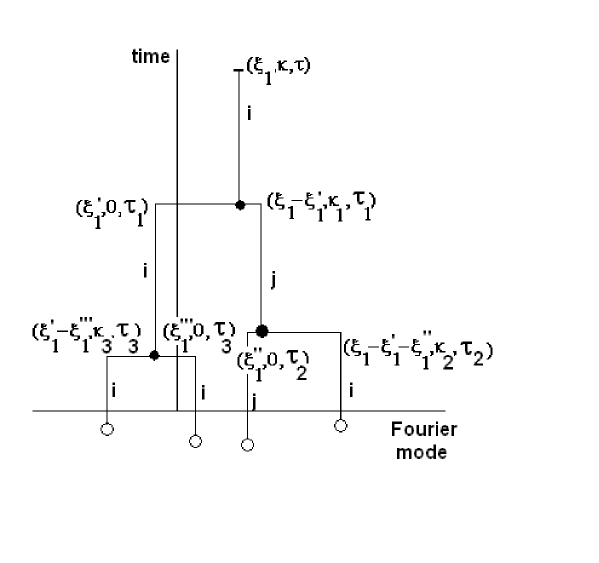
Figure 1: A sample path of the stochastic process I

and

$$\begin{array}[]{lll}k&=&\xi_{2}\\ k_{1}&=&k+\left(\tau-\tau_{1}\right)\frac{\xi_{1}}{\gamma\left(\left|\xi_{2}\right|\right)}\\ k_{2}&=&k_{1}+\left(\tau_{2}-\tau_{1}\right)\frac{\left(\xi_{1}-\xi_{1}^{{}^{\prime}}\right)}{\gamma\left(\left|k_{1}\right|\right)}\\ k_{3}&=&\left(\tau_{3}-\tau_{1}\right)\xi_{1}^{{}^{\prime}}\end{array}$$ (19)

With the conditions (A) and (B), choosing

$$\lambda\geq\left|\frac{8\pi e_{i}e_{j}}{\min_{i}\left\{m_{i}\right\}}\right|$$ (20)

and

$$c\leq e^{-\lambda\tau}\frac{1}{3\pi}$$ (21)

the absolute value of all coupling constants is bounded by one. The branching process, being identical to a Galton-Watson process, terminates with probability one and the number of inputs to the functional is finite (with probability one). With the bounds on the coupling constants, the multiplicative functional is bounded by one in absolute value almost surely.

Once a stochastic representation is obtained for $\chi\left(\xi_{1},\xi_{2},\tau\right)$, one also has, by (8), a stochastic representation for the solution of the Fourier-transformed Poisson-Vlasov equation and one obtains:

Proposition 1. The process I, above described, provides a stochastic representation for the Fourier-transformed solutions of the Poisson-Vlasov equation $F_{i}\left(\xi_{1},\xi_{2},t\right)$ for any arbitrary finite value of the arguments, provided the initial conditions at time zero satisfy the boundedness conditions (A).

So far we have constructed a general process that provides a stochastic representation for the interacting Vlasov equation, not only for the Poisson case, but also for more general situations with quadratic nonlinearities. However, because of the integrated nature of the Coulomb interaction, the Poisson case is special in that there is also a representation by a simpler process. Looking at equation (9) one sees that because of the factor $\stackrel{{\scriptstyle\rightarrow}}{{\xi_{2}}}\cdot\stackrel{{\scriptstyle\wedge}}{{\xi_{1}^{{}^{\prime}}}}$ only the trees where the mode $\chi_{j}\left(\xi_{1}^{{}^{\prime}},0,\tau-s\right)$ survives until time zero will contribute to the functional. That is, the only trees with non-zero contributions to the functional (17) are the one-sided trees represented in Fig.2. Therefore for the calculation of the solution one may replace $\chi_{j}\left(\xi_{1}^{{}^{\prime}},0,\tau-s\right)$ by the initial condition computed at $\left(\xi_{1}^{{}^{\prime}},\left(\tau-s\right)\xi_{1}^{{}^{\prime}}\right)$. The process then becomes the following linear process with random couplings

$$X_{i}^{\left(k+1\right)}\left(\xi_{1},\xi_{2},\tau\right)$$

$$= \chi_{i}\left(\xi_{1},\xi_{2}+\tau\frac{\xi_{1}}{\gamma\left(\left|\xi_{2}\right|\right)},0\right)\mathbf{1}_{\left[s>\tau\right]}$$

$$+g_{ii}^{{}^{\prime}}\left(\xi_{1},\xi_{1}^{{}^{\prime}},s\right)X_{i}^{\left(k\right)}\left(\xi_{1}-\xi_{1}^{{}^{\prime}},\xi_{2}+s\frac{\xi_{1}}{\gamma\left(\left|\xi_{2}\right|\right)},\tau-s\right)\mathbf{1}_{\left[s<\tau\right]}\mathbf{1}_{\left[l_{s}=0\right]}$$

$$+g_{ij}^{{}^{\prime}}\left(\xi_{1},\xi_{1}^{{}^{\prime}},s\right)X_{i}^{\left(k\right)}\left(\xi_{1}-\xi_{1}^{{}^{\prime}},\xi_{2}+s\frac{\xi_{1}}{\gamma\left(\left|\xi_{2}\right|\right)},\tau-s\right)\mathbf{1}_{\left[s<\tau\right]}\mathbf{1}_{\left[l_{s}=1\right]}$$

the coupling constant at the branchings being

$$g_{ij}^{{}^{\prime}}\left(\xi_{1},\xi_{1}^{{}^{\prime}},s\right)=-\frac{8\pi e_{i}e_{j}}{m_{i}\lambda}\frac{\left(\left|\xi_{1}^{{}^{\prime}}\right|^{-1}h*h\right)\left(\xi_{1}\right)}{h\left(\xi_{1}\right)}\frac{\stackrel{{\scriptstyle\rightarrow}}{{\xi_{2}}}\cdot\stackrel{{\scriptstyle\wedge}}{{\xi_{1}^{{}^{\prime}}}}}{\gamma\left(\left|\xi_{2}\right|\right)}\chi_{j}\left(\xi_{1}^{{}^{\prime}},\left(\tau-s\right)\xi_{1}^{{}^{\prime}},0\right)$$ (23)

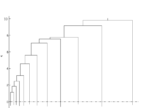
Figure 2: A one-sided tree corresponding to process II

The functional representing the solution is the product of all branching coupling constants times one additional factor corresponding to the last non-branching mode. The result is the following

Proposition 2. The linear process II, defined by (2) and (23) also provides a stochastic representation of the solutions of the Poisson-Vlasov equation, the conditions on the kernels and initial conditions being given by (A), (12) and (20).

3 Stochastic representation and numerical codes

The backwards-in-time probabilistic representations, obtained in Sect.2, seem appropriate for the numerical evaluation of Fourier-localized solutions. Good statistics requires the average of the multiplicative functional over many realization trees. In the backwards in time realization one fixes a particular mode at time $\tau$ and generates as many trees as needed for that particular mode. Notice that by studying high Fourier modes one may obtain information about the small scale behaviour of the solution without having the need for a fine grid as it would be necessary in a real space numerical code. Each realization tree being independent of all the others, the probabilistic code is also appropriate for parallelization.

We will not report, in this paper, extensive calculations using these representations and the corresponding codes. Nevertheless we list all the needed probability distributions needed to implement the method.

For the construction of the sample trees and the calculation of the functional, the following probability densities are needed:

- The probability of a $\xi_{1}-$ mode branching into $\xi_{1}^{{}^{\prime}}$ and $\xi_{1}-\xi_{1}^{{}^{\prime}}$ modes

$$p\left(\xi_{1},\xi_{1}^{{}^{\prime}}\right)=\frac{\left|\xi_{1}^{{}^{\prime}}\right|^{-1}\left(1+\left|\xi_{1}-\xi_{1}^{{}^{\prime}}\right|^{2}\right)^{-2}\left(1+\left|\xi_{1}^{{}^{\prime}}\right|^{2}\right)^{-2}}{\Gamma\left(\left|\xi_{1}\right|\right)}$$ (24)

with $\Gamma\left(\xi_{1}\right)$ given by Eq.(13). One notices that, for each $\left|\xi_{1}\right|$, this probability is only function of two variables, the $\left|\xi_{1}^{{}^{\prime}}\right|$ and the angle between $\xi_{1}$ and $\xi_{1}^{{}^{\prime}}$. Therefore defining

$$z=\frac{1}{1+\left|\xi_{1}^{{}^{\prime}}\right|^{2}}$$ (25)

and changing the integration measure one obtains a

- Probability density $p\left(z,\cos\theta\right)$

$$p\left(z,\cos\theta\right)=\frac{\pi}{\Gamma\left(\left|\xi_{1}\right|\right)}\frac{1}{\left(\left|\xi_{1}\right|^{2}+\frac{1}{z}-2\left|\xi_{1}\right|\cos\theta\sqrt{\frac{1}{z}-1}\right)^{2}}$$ (26)

with $z$ in the interval $\left(0,1\right)$ and $\cos\theta$ in the interval $\left(-1,1\right)$.

Because the inverse of the cumulative distribution functions have not a nice analytic form, we may use the reject method in the plane $\left(z,\cos\theta\right)$ to simulate this probability distribution. For this, one needs

$$p\left(z,\cos\theta\right)_{\max}=\frac{\pi}{\Gamma\left(\left|\xi_{1}\right|\right)}$$ (27)

which is obtained for $\cos^{2}\theta=1$ and $\frac{1}{z}=\left|\xi_{1}\right|^{2}+1$.

However because $p\left(z,\cos\theta\right)_{\max}$ is very large for large $\left|\xi_{1}\right|$ in a narrow region, it is more efficient to use

- The integrated $p\left(z\right)$ density,

$$p\left(z\right)=\frac{2\pi}{\Gamma\left(\left|\xi_{1}\right|\right)}\frac{1}{\left(\left|\xi_{1}\right|^{2}-\frac{1}{z}\right)^{2}+4\left|\xi_{1}\right|^{2}}$$ (28)

with $p\left(z\right)_{\max}=p\left(\min\left(\left|\xi_{1}\right|^{-2},1\right)\right)$, to choose $z$ and then, once $z$ is chosen, to use

- The conditional probability density $p\left(\cos\theta|z\right)$

$$p\left(\cos\theta|z\right)=\frac{\left(\left|\xi_{1}\right|^{2}-\frac{1}{z}\right)^{2}+4\left|\xi_{1}\right|^{2}}{2\left(\left|\xi_{1}\right|^{2}+\frac{1}{z}-2\left|\xi_{1}\right|\cos\theta\sqrt{\frac{1}{z}-1}\right)^{2}}$$ (29)

with

$$\max_{\theta}p\left(\cos\theta|z\right)=\frac{\left(\left|\xi_{1}\right|^{2}-\frac{1}{z}\right)^{2}+4\left|\xi_{1}\right|^{2}}{2\left(\left|\xi_{1}\right|^{2}+\frac{1}{z}-2\left|\xi_{1}\right|\sqrt{\frac{1}{z}-1}\right)^{2}}$$ (30)

to choose $\cos\theta$.

Once $z$ and $\cos\theta$ are chosen, one computes $\left|\xi_{1}^{{}^{\prime}}\right|=\sqrt{\frac{1}{z}-1}$ and chooses

$$\varphi=2\pi RAND$$

RAND being a random variable uniformly distributed in the interval $\left(0,1\right)$. Then one obtains

$$\xi_{1}^{{}^{\prime}}=\left|\xi_{1}^{{}^{\prime}}\right|\left(\sin\theta\cos\varphi,\sin\theta\sin\varphi,\cos\theta\right)$$

and $\xi_{1}-\xi_{1}^{{}^{\prime}}$.

Notice that only the amplitudes of the Fourier modes $\left|\xi_{1}^{{}^{\prime}}\right|$ and $\left|\xi_{1}-\xi_{1}^{{}^{\prime}}\right|$ are needed as inputs to compute the probabilities in the next branchings but the full vector is needed to compute $\xi_{2}$. Finally the lifetime $\tau$ of each mode is obtained from

$$\tau=\frac{\ln\left(RAND\right)}{\lambda}$$ (31)

For the trees a standard indexation is used, each tree being a row vector of integer numbers with the number $k$ at the position $n$ meaning that that mode was born at the branching of the mode in the position $k$.

The conditions (A), (12) and (20) guarantee that all factors entering the multiplicative functional (17) are bounded by one, implying that the functional itself is also bounded. This, together with the Galton-Watson nature of the branching, insures convergence of the expectation value. However, in practice, this leads to very small values of the functional and for large times (large trees) one may be faced with round-off inaccuracies in the computer. In fact the limitation to factors strictly not larger than one is only imposed for mathematical convenience. What is actually needed for convergence is that the functional be bounded by some value with probability one. A more relaxed condition on the constants may therefore be obtained by imposing $\left|p_{n}g_{\max}^{n}\left(I\right)F_{\max}^{n+1}\right|<M$ for process I and $\left|p_{n}g_{\max}^{n}\left(II\right)F_{\max}\right|<M$ for process II, $p_{n}$ being the probability of a tree with $N$ branchings, $g_{\max}^{n}\left(I\right)$ and $g_{\max}^{n}\left(II\right)$ the maximum values of the couplings and $F_{\max}$ the maximum value of the initial condition.

To test the method we have studied the time evolution of small and large Fourier modes in a plasma with two particle species of opposite charges, one light and the other heavy, with two types of initial Fourier distribution functions, namely

$$F_{i}^{(1)}\left(\xi_{1},\xi_{2},0\right)=C_{0}^{(1)}e^{-\gamma\left|\xi_{1}\right|^{2}}e^{-\beta_{i}\left|\xi_{2}\right|^{2}}$$ (32)

and

$$\begin{array}[]{lll}F_{+}^{(2)}\left(\xi_{1},\xi_{2},0\right)&=&C_{0+}^{(2)}e^{-\gamma\left|\xi_{1}\right|^{2}}e^{-\beta_{+}\left|\xi_{2}\right|^{2}}\\ F_{-}^{(2)}\left(\xi_{1},\xi_{2},0\right)&=&C_{0-}^{(2)}e^{-\gamma\left|\xi_{1}\right|^{2}}\theta\left(k-\left|\xi_{2}\right|^{2}\right)\end{array}$$ (33)

$\beta_{+}=40\beta_{-}$ and the $C_{0}^{(i)\prime}s$ are chosen to fulfill condition (A). For the initial condition we have chosen $\xi_{1}=\left(0.01,0.01,0.01\right)$ and varied $\left|\xi_{2}\right|^{2}$ in the range $3.10^{-4}$ to $7$. Then, the time evolution is computed using the one-sided representation (process II). Some results are shown in Figs.3 and 4, with time in units of $\frac{1}{\lambda}$. Although it is known that on $\mathbb{R}^{3}$ and without an external force there are no nontrivial steady states when both charges of opposite sign can move[11] [12], one can see the relative stability of the Fourier modes for short times for the Gaussian initial condition $F^{\left(1\right)}$, whereas for the $F^{\left(2\right)}$ initial condition one sees the appearance of growing Fourier modes that were not present in the initial density. Although the points were computed for the same set of final $\tau^{\prime}s$, in the plots we show the actual time $t$, obtained from (5).

Figure 3: Time evolution of some Fourier modes for the $F^{\left(1\right)}$ initial condition, $T=\lambda t$

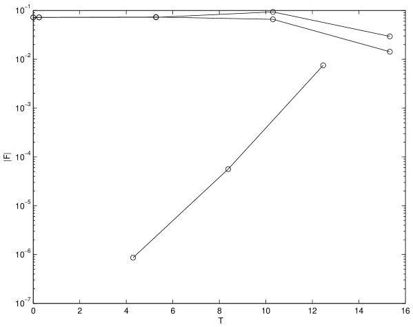
Figure 4: Time evolution of some Fourier modes for the $F^{\left(2\right)}$ initial condition, $T=\lambda t$

Notice that to obtain a reasonable stability of the averaged functional one needs to compute many sample trees. The points shown in the figures were obtained with averages over $10^{6}$ or $2\times 10^{6}$ trees, depending on the evolution time. The reason for the need for a large number of sample trees arises from the fact that, for large times, most trees contribute a very small value to the average, the actual average arising from the contribution of a small number of them. This calls for the need to control the results by a large deviation analysis (see below).

4 Conclusions

1 - Mostly when localized solutions in Fourier space (or in configuration space for other stochastic representations) are desired, the method seems appropriate. When a global calculation of the solution is desired, the stochastic representation method is probably not competitive with other current simulation methods. The computational example presented in Sect. 3, merely illustrative of the method, was obtained with modest computational means. Our purpose was mostly to test the stability of the results. To obtain good statistics and also to study the fluctuation spectrum of the process, many sample trees have to be used for each initial condition. However, because each tree is independent from the others and also because after the branching each mode evolves independently of the others, this algorithm is well suited for parallelization and distributed computing. In this sense the stochastically-based algorithms might also become competitive even for global calculations using parallel computing. In fact stochastic representations have already been found to be efficient for domain decomposition in parallel computing [13] [14].

2 - The fluctuations around the mean in a branching process are typically very much non-Gaussian. Therefore a simple calculation of the standard deviation or other lower order momenta are not sufficient to check the reliability of the results. A large deviation analysis is recommended for numerical calculations using branching processes. Some general results on large deviations in branching processes are known[15] [16] [17] [18]. Of more practical importance are probably methods to estimate large deviation effects directly from the data. This may be done, for example, by the empirical construction of the deviation function. This is done by the empirical construction of the free energy and from it, by Legendre transform, the deviation function. For details we refer to [19]. Given a deviation function $I\left(x\right)$, the probability of obtaining a value $x$ for the empirical average of a sample of size $n$ is

$$P_{n}\left(dx\right)\asymp e^{-nI\left(x\right)}dx$$

where $\asymp$ means logarithmic equivalence. We have used the method described in [19] to check the reliability of the results. In the Fig.5 we present the empirically obtained deviation function for a sample of $5\times 10^{5}$ trees. At first sight the regular behavior of $I\left(y\right)$ around the mean, seen in the upper plot of Fig.5, would seem to indicate that the distribution is Gaussian. However expanding a little more (in the lower plot) the domain of the variable $x$ one sees the very non-Gaussian nature of the data. It means that, had we used a smaller sample, any empirical mean in the range $0.04-0.075$ would have been likely. A rough lower bound on the size of the needed sample may be obtained from the inverse of the deviation function at the point where the behavior of $I\left(x\right)$ changes.

Figure 5: The behavior of the deviation function for a sample of size $5\times 10^{5}$

3 - Stochastic representations of the solutions of deterministic equations may have some relevance for the study of the fluctuation spectrum. In the past, the fluctuation spectrum of charged fluids was studied either by the BBGKY hierarchy derived from the Liouville or Klimontovich equations, with some sort of closure approximation, or by direct approximations to the N-body partition function or by models of dressed test particles, etc. (see reviews in [20] [21]). Alternatively, by linearizing the Vlasov equation about a stable solution and diagonalizing the Hamiltonian, a canonical partition function may be used to compute correlation functions [22].

As a model for charged fluids, the Vlasov equation is just a mean-field collisionless theory. Therefore, it is unlikely that, by itself, it will contain full information on the fluctuation spectrum. Kinetic and fluid equations are obtained from the full particle dynamics in the 6N-dimensional phase-space by a chain of reductions. Along the way, information on the actual nature of fluctuations and turbulence may have been lost. An accurate model of turbulence may exist at some intermediate (mesoscopic) level, but not necessarily in the final mean-field equation.

When a stochastic representation is constructed, one obtains a process for which the mean value is the solution of the mean-field equation. The process itself contains more information. This does not mean, of course, that the process is an accurate mesoscopic model of Nature, because we might be climbing up a path different from the one that led us down from the particle dynamics. Nevertheless, insofar as the stochastic representation is qualitatively unique and related to some reasonable iterative process, it provides a surrogate mesoscopic model from which fluctuations are easily computed. This is what we have referred elsewhere as the stochastic principle [10]. At the minimum, one might say that the stochastic principle provides yet another closure procedure for the kinetic equations.

References

• [1] R. Courant, K. Friedrichs and H. Lewy; Mat. Ann. 100 (1928) 32-74.
• [2] H. P. McKean; Comm. Pure Appl. Math. 28 (1975) 323-331, 29 (1976) 553-554.
• [3] E. B. Dynkin; Prob. Theory Rel. Fields 89 (1991) 89-115.
• [4] E. B. Dynkin; Diffusions, Superdiffusions and Partial Differential Equations,AMS Colloquium Pubs., Providence 2002.
• [5] Y. LeJan and A. S. Sznitman ; Prob. Theory and Relat. Fields 109 (1997) 343-366.
• [6] E. C. Waymire; Prob. Surveys 2 (2005) 1-32.
• [7] R. N. Bhattacharya et al. ; Trans. Amer. Math. Soc. 355 (2003) 5003-5040
• [8] M. Ossiander ; Prob. Theory and Relat. Fields 133 (2005) 267-298.
• [9] R. Vilela Mendes; Zeitsch. Phys. C54, (1992) 273-281.
• [10] R. Vilela Mendes and F. Cipriano; A stochastic representation for the Poisson-Vlasov equation, arXiv:physics/0611186, Commun. Nonlinear Science and Num. Simul. http://dx.doi.org/10.1016/j.cnsns.2007.05.008
• [11] R. Illner and G. Rein; Math. Meth. in Appl. Sci. 19 (1996) 1409-1413.
• [12] P. Braasch, G. Rein and J. Vukadinovic; SIAM J. Appl. Math. 59 (1998) 831-844.
• [13] J. A. Acebrón, M. P. Busico, P. Lanucara and R. Spigler; SIAM J. Sci. Comput. 27 (2005) 440-457.
• [14] J. A. Acebrón and R. Spigler; Lect. Notes in Comput. Sci. and Eng. 55 (2007) 475-480.
• [15] J. D. Biggins and N. H. Bingham; Adv. in Appl. Probability 25 (1993) 757-772.
• [16] K. B. Athreya; The Annals of Applied Probability 4 (1994) 779-790.
• [17] P. E. Ney and A. N. Vidyashankar; The Annals of Applied Probability 14 (2004) 1135-1166.
• [18] K. Fleischmann and V. Wachtel; arXiv:math.PR/0605617.
• [19] J. Seixas and R. Vilela Mendes; Nucl. Phys. B383 (1992) 622-642.
• [20] C. R. Oberman and E. A. Williams; in Handbook of Plasma Physics (M. N. Rosenbluth, R. Z. Sagdeev, Eds.), pp. 279-333, North-Holland, Amsterdam 1985.
• [21] J. A. Krommes; Phys. Reports 360 (2002) 1-352.
• [22] P. J. Morrison; Phys. of Plasmas 12 (2005) 058102.