Accretion of Low Angular Momentum Material onto Black Holes: Radiation Properties of Axisymmetric MHD Flows.

Context: Numerical simulations of MHD accretion flows in the vicinity of a supermasssive black hole provide important insights to the problem of why and how systems – such as the Galactic Center – are underluminous and variable. In particular, the simulations indicate that low angular momentum accretion flow is strongly variable both quantitatively and qualitatively. This variability and a relatively low mass accretion rate are caused by an interplay between a rotationally supported torus, its outflow and a nearly non-rotating inflow.

Aims: To access applicability of such flows to real objects, we examine the dynamical MHD studies with computations of the time dependent radiation spectra predicted by the simulations.

Methods: We calculate synthetic broadband spectra of accretion flows using Monte Carlo techniques. Our method computes the plasma electron temperature allowing for the pressure work, ion-electron coupling, radiative cooling, and advection. The radiation spectra are calculated by taking into account thermal synchrotron and bremsstrahlung radiation, self absorption, and Comptonization processes. We also explore effects of non-thermal electrons. We apply this method to calculate spectra predicted by the time-dependent model of an axisymmetic MHD flow accreting onto a black hole presented by Proga and Begelman.

Results: Our calculations show that variability in an accretion flow is not always reflected in the corresponding spectra, at least not in all wavelengths. We find no one-to-one correspondence between the accretion state and the predicted spectrum. For example, we find that two states with different properties – such as the geometry and accretion rate – could have relatively similar spectra. However, we also find two very different states with very different spectra. Existence of nonthermal radiation may be necessary to explain X-rays flaring because thermal bremsstrahlung, that dominates X-ray emission, is produced at relatively large radii where the flow changes are small and slow.

1 Introduction

The overall radiative output from the Galactic center (GC) is very low for a system hosting a supermassive black hole (SMBH). This under-performance of the nearest SMBH challenges our understanding of mass accretion processes.

Certain properties of GC are relatively well established. For example, the existence of a $\sim 3.7\times 10^{6}\leavevmode\nobreak\ \rm M_{\odot}$ SMBH in GC is supported by the stellar dynamics (e.g. Schoedel et al. 2002, Ghez et al. 2003). The nonluminous matter within 0.015 pc of GC is associated with Sgr A^∗, a bright compact radio source (Balick & Brown 1974). Observations of Sgr A^∗ in X-ray and radio bands reveal a luminosity substantially below the Eddington limit, $L_{\rm Edd}=3\times 10^{44}$ erg s^-1. In particular, Chandra observations show a luminosity in 2-10 keV X-rays of $\approx 2\times 10^{33}$ erg s^-1, ten orders of magnitude below $L_{\rm Edd}$ (Baganoff et al. 2003). Chandra observations also revealed an X-ray flare rapidly rising to a level about 45 times as large, lasting for only $\sim 10^{4}$ s, indicating that the flare must originate near the black hole  (Baganoff et al. 2001; Baganoff et al. 2003). A strong variability of Sgr A^∗ was also observed in radio and near-infrared (e.g., Eckart et al. 2005).

Despite a relative wealth of the observational data and significant theoretical developments, a character of the accretion flow in GC is poorly understood. In particular, it is unclear whether the emission comes from inflowing or outflowing material (e.g., Markoff et al. 2001; Yuan, Markoff, Falcke 2002). Although the accretion fuel is most likely captured from the stellar winds, mass accretion rate $\dot{M}_{a}$ onto the central black hole is uncertain. For example, the quiescent X-ray emission measured with Chandra implies $\dot{M}_{a}\sim$ a few $\times 10^{-6}\leavevmode\nobreak\ \rm M_{\odot}\,yr^{-1}$ at $\sim 10^{5}R_{g}$ (assuming spherically symmetric Bondi accretion Baganoff et al. 2003) whereas the measurements of the Faraday rotation in the millimeter band imply $\dot{M}_{a}\leavevmode\nobreak\ \sim$ a few $\times 10^{-7}-10^{-8}\leavevmode\nobreak\ \rm M_{\odot}\,yr^{-1}$ (Bower et al. 2003, 2005). Recent measurements of Faraday rotation of Marrone et al. (2006) imply even lower mass accretion rate $\sim 10^{-7}-10^{-9}\leavevmode\nobreak\ \rm M_{\odot}\,yr^{-1}$, where the lower limit is valid for sub-equipartition disordered or toroidal magnetic field.

An increasing amount of the available observational data of the Galactic Center has motivated a recent development in the theory and simulations of accretion flows. Most theoretical work has been focused on steady state models, which assume that the specific angular momentum, $l$, is high and the inflow proceeds through a form of the so-called radiatively inefficient accretion flow (RIAF; e.g., Narayan et al. 1998; Blandford & Begelman 1999; Stone, Pringle & Begelman 1999; Quataert & Gruzinov 2000; Stone & Pringle 2001). A high specific angular momentum considered in these studies is a reasonable assumption but not necessarily required by the data. In fact, many observational aspects of Sgr A^∗ can be better explained by low-$l$ accretion flows. For example, Moscibrodzka (2006, hereafter M06) showed that models of purely spherical accretion flows underpredict the total observed luminosity if the flow radiative efficiency is not arbitrarily adopted but calculated self-consistently from the synchrotron, bremsstrahlung, and Compton emission of the accreting material. M06’s results imply that low-$l$ flows can also reproduce the observed total luminosity as good as the high-$l$ flows. Additionally, the intrinsic time variability of low-$l$ magnetized flows found by Proga & Begelman (2003, PB03 hereafter) can naturally account for some of Sgr A^∗ variability (Proga 2005).

In this paper, we present synthetic continuum spectra and Faraday rotation measurements (RM) calculated based on time-dependent two-dimensional (2-D) axisymmetric MHD simulations of accretion flows performed PB03. PB03’s simulations are for slowly rotating flows and are complementary to other simulations which considered strongly rotating accretion flows set to be initially pressure-rotation supported torii (e.g., Stone & Pringle 2001; Hawley & Balbus 2002 (hereafter HB02); Krolik & Hawley 2002; Igumenshchev & Narayan 2002). PB03 attempt to mimic the outer boundary conditions of classic Bondi accretion flows modified by the introduction of a small, latitude-dependent angular momentum at the outer boundary, a pseudo-Newtonian gravitational potential, and weak poloidal magnetic fields. Such outer boundary conditions allow for the density distribution at infinity to approach spherical symmetry. Recent X-ray images taken by the Chandra show that the gas distribution in the vicinity of a SMBH at the centers of nearby galaxies is close to spherical (e.g., Baganoff et al. 2003; Di Matteo et al. 2003; Fabbiano et al. 2003). Thus the outer boundary considered by PB03 capture better RIAF in Sgr A^∗ than those used in simulations of high-$l$ flows.

PB03’s simulations follow the evolution of the material with a range of $l$. The material with $l\gtrsim 2cR_{S}$ (where $R_{S}=\frac{2GM}{c^{2}}$ is Schwarzschild radius) forms an equatorial torus because its circularization radius is located outside the last stable orbit. The torus accretes onto a black hole as a result of magnetorotational instability (MRI, Balbus & Hawley 1991). As the torus accretes, it produces a corona and an outflow which can be strong enough to prevent accretion of a low-$l$ material (i.e., with $l<2cR_{S}$) to fall through the polar regions. The torus outflow and the corona can narrow or even totally close the polar funnel for the accretion of low-$l$ material. One of PB03’s conclusions is that even a slow rotational motion of the MHD flow at large radii can significantly reduce $\dot{M}_{a}$ compared to the Bondi rate.

Many properties of the torus found by PB03 are typical for the MHD turbulent torii presented in other global MHD simulations (e.g., Stone & Pringle 2001; HB02). Radial density profiles, properties of the corona and outflow, as well as rapid variability are quite similar in spite of different initial and the outer boundary conditions.

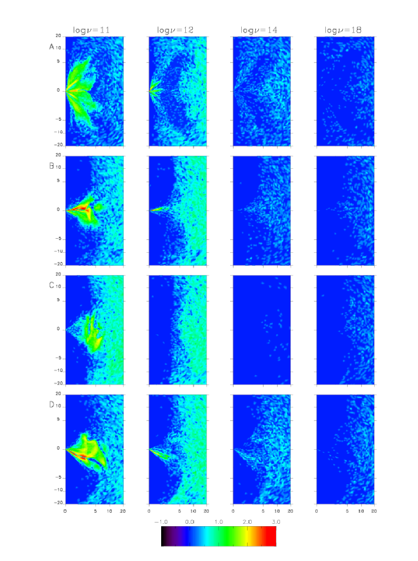
Figure 2: 2-D color maps of the emission at four frequencies: $\log\nu=$11,12,14, and 18 Hz (from left to the right) and for four distinct accretion sates A,B,C,and D (from top to bottom; see the main text for more detail on state A,B,C, and D). Length scale for the horizontal axies is logarithmic in units of $R_{in}$, so that the size of a box is 20 $R_{S}$.

The main difference between simulations of PB03’ and the others is that the former showed that the typical torus accretion can be quasi-periodically supplemented or even replaced by a stream-like accretion of the low-$l$ material occurring outside the torus (e.g., see the bottom right panel of Fig. 2 in PB03). When this happens, $\dot{M}_{a}$ sharply increases and then gradually decreases. The mass-accretion rate due to this ’off torus’ inflow can be one order of magnitude larger than that from the torus itself (see Fig. 1 in PB03). The off torus accretion is a consequence of the outer boundary and initial conditions which introduce the low-$l$ material to the system. This material can reach a black hole because the torus, the corona, and the outflow are not always strong enough to push it away.

One can expect that in the vicinity of SMBH at the centers of galaxies, some gas has a very little angular momentum and could be directly accreted. Such a situation likely occurs in GC where a cluster of young, massive stars losing mass surrounds a SMBH (e.g., Loeb 2004; Moscibrodzka et al. 2006, Rockefeller et al. 2004). On the other hand, 3D hydrodynamical numerical models of wind from the close stars showed that the wind can form a cold disk around the Sgr A* with the inner radius of $10^{3}-10^{4}$ Schwarzschild radii $R_{S}$ (Cuadra et al. 2006). But unless the disk includes the viscosity it can not accrete closer. In the context of such models we can again expect that only a matter with initial relatively low angular momentum, can inflow at smaller radii at which PB03 started their computations. Also the winds from inner 0.5 ” stars (SO-2, SO-16, SO-19) can supply a lower angular momentum matter for the accretion (Loeb 2004). To test further properties of the low angular momentum scenario, we supplement here the dynamical MHD study of PB03 with the computations of the time dependent radiation spectra of accreting/outflowing material.

There are only a few papers (HB02; Goldston et al. 2005; Ohsuga et al. 2005) estimating radiation spectra, or at least the integrated emission, predicted by MHD simulations of accretion flows in GC. These papers assumed different dynamical situations than the one considered in the PB03 simulations. HB02 made an order-of-magnitude estimates of the emission emerging from a MHD torus in the Galactic Center. In particular, they estimated the peak frequency of the synchrotron emission coming from the inner parts of the flow at $\leavevmode\nobreak\ 2.5\times 10^{11}(n_{0}/10^{8})^{1/2}$ Hz (where $n_{0}$ is the scaling density of the ions). They also calculated a location of the peak of a total bremsstrahlung emission at about $10^{21}$ Hz. They concluded that the dynamical variability in the MHD simulations is in general consistent with the observed variation in Sgr A*. However, HB02 focused mainly on a dynamical evolution of a high-$l$ non-radiative torus and did not consider the detailed spectral properties of the flow.

Goldston et al. (2005) used numerical simulation of HB02 and estimated the synchrotron radiation assuming the scaling of the electron temperature, $T_{e}\sim T_{i}$. They calculated the synchrotron part of the radiation spectrum and modeled polarization variability including effects of self-absorption. The emission is variable (by a factor of 10) at optically thin radio frequencies and originates in the very inner parts of the flow (timescales of order of hours). The authors predict that the variability at different frequencies should be strongly correlated. The general conclusion is that a variable synchrotron emission in Sgr A* could be generated by a turbulent magnetized accretion flow.

Ohsuga et al. (2005) presented spectral features predicted by the 3D MHD flows simulated by Kato et al. (2004). These simulations followed an evolution of a turbulent torus. The heating/cooling balance equation used by Ohsuga et al. (2005) for calculating the electron temperature includes radiative cooling and heating via Coulomb collisions. The authors found that MHD flows in general overestimate the X-ray emission in Sgr A*, because the bremsstrahlung radiation originated at large radii dominates the X-ray band. However, the quiescent state spectrum of Sgr A* cannot be reconstructed simultaneously in the radio and X-ray bands. The authors reconstructed the observed flaring state, with assumption of rather high $\dot{M}_{a}$ and restrict the size of the emission region to only 10 $R_{S}$. A small size of the emission region is consistent with the short duration of the observed X-ray flares, and it results in the X-ray variability so there is no need for additional radiation processes, e.g. radiation from nonthermal particles. On the other hand the observed quiescent X-ray emission is extended, which contradicts the assumption made in Ohsuga et al. (2005).

Our goal is to compute the spectral signatures of a highly time-dependent flow found by PB03. In particular, we check whether a reoccurring switching between various accretion modes present in the PB03 simulations is consistent with the observed flare activity in Sgr A*. Our spectral model assumes that at each moment of the accretion flow there is a stationary distribution of both hydrodynamical and magnetic quantities. Radiative transfer is calculated based on this ’stationary’ solution. The radiation computations are performed independently from the dynamics (Sec.2). Our results show which parts of the accretion flow create characteristic features in the radiation spectra. In particular, we create maps of emission for synchrotron radiation including self-absorption and Comptonization (Sec.3). We also show time evolution of the spectra emerging from the flow for a number of moments in the evolution of an inner torus. In section 3 we discussed results in the context of the Galactic Center. We conclude in Sec.4.

2 Method

We computed the synthetic spectra for the simulation denoted as ’run D’ in PB03. This simulation assumed a slowly rotating accretion flow (with an angular momentum parameter $l\sim 2R_{S}c$ at the equatorial plane) and were performed in the spherical polar coordinates. The computational domain for run D was defined to occupy the radial range $r_{i}\leavevmode\nobreak\ =\leavevmode\nobreak\ 1.5\leavevmode\nobreak\ R_{S}\leq r\leq\ r_{o}\leavevmode\nobreak\ =\leavevmode\nobreak\ 1.2\leavevmode\nobreak\ R_{B}$, (where $R_{B}=\frac{GM}{c^{2}_{\infty}}$ is the Bondi radius, $c_{\infty}$ is a sound speed at infinity ), and the angular range $0^{\circ}\leq\theta\leq 180^{\circ}$. PB03 considered models with $R^{\prime}_{S}\equiv R_{S}/R_{B}=10^{-3}$. The $r-\theta$ domain was discretized into zones with 140 zones in the $r$ direction and 100 zones in the $\theta$ direction. PB03 fixed the zone size ratios, $dr_{k+1}/dr_{k}=1.05$, and $d\theta_{l}/d\theta_{l+1}=1.0$ for $0^{\circ}\leq\theta\leq 180^{\circ}$.

The MHD simulation were performed using dimensionless variables. Therefore we first rescale all the quantities. The gas density, $\rho$ is scaled by a multiplication factor $\rho_{\infty}$ which is the density at infinity. The magnetic field scales with $[(B_{r}^{2}+B_{\theta}^{2}+B_{\phi}^{2})\rho_{\infty}]^{1/2}$, where $B_{r},B_{\theta}$, and $B_{\phi}$ is the radial, latitudinal, and azimuthal component of the magnetic field respectively. The internal energy density, $e$ scales with $\rho_{\infty}$ and $c_{\infty}$.

To compute the synchrotron emissivity we calculate the strenght of the magnetic field, $B=(B_{r}^{2}+B_{\theta}^{2}+B_{\phi}^{2})^{1/2}$, at each grid point.

The ion temperature of the gas is calculated using politropic relation: $T_{i}=\frac{\mu m_{h}e(\gamma-1)}{k_{b}\rho}$, where $k_{b}$, $\mu$, and $m_{h}$ is the Boltzmann constant, mean particle weight ($\mu=0.5$) and proton mass, respectively. We set the adiabatic index $\gamma=5/3$. We use scaling constants appropriate for the case of Sgr A* i.e. $\rho_{\infty}$ is chosen to fit the observed mass accretion rate (see Section 3.1).

PB03 did not include radiative cooling in their calculations; therefore, we use $e$ and $\rho$ to compute the distribution of the temperature of ions $T_{i}$, using the politropic relation mentioned above. However, determination of the electron temperature is the key step in spectral calculations. Ions and electrons undergo different types of cooling and heating processes, and they are not well coupled in a low density plasma. Ions and electrons are likely to have different temperatures. We calculate the electron temperature distribution by solving the heating-cooling balance at each grid point at a given time in the simulation. We present a detailed description of the method in Sect.2.1 and outline the radiative transfer method in Sect. 2.2.

2.1 Heating-cooling balance.

To calculate the electron temperature in each cell of the grid, we solve the cooling-heating balance equation for electrons which is given by:

$$Q_{{\rm adv}}=\delta Q_{{\rm pdv}}+Q_{{\rm ie}}-Q_{{\rm cooling}},$$ (1)

where $Q_{{\rm adv}}$, $Q_{{\rm pdv}}$,$Q_{{\rm ie}}$, and $Q_{{\rm cooling}}$ is the advective energy transport, compression heating of the ions, ion-electron Coulomb collision term, and radiative cooling, respectively. The numerical factor, $\delta$ is defined as the fraction of the compression energy that directly heats electrons ( $0\leq\delta\leq 0.5$).

The advection term, $Q_{adv}$ consist of the radial part, shown for example in Narayan et al. (1998), which can be expressed by:

$$Q_{adv,r}=\frac{\rho k_{B}v_{r}}{\mu m_{H}}\Big{[}\frac{3(3-\beta)}{\beta}+a(T_{e})+T_{e}\frac{da(T_{e})}{dT_{e}}\Big{]}\frac{dT_{e}}{dr}$$

$$-\frac{v_{r}k_{B}T_{e}}{\beta\mu m_{H}}\frac{d\rho}{dr}$$ (2)

in 2D, a term in $\theta$ direction should be added. This is a small modification of the radial one:

$$Q_{adv,\theta}=\frac{\rho k_{B}v_{\theta}}{\mu m_{H}r}\Big{[}\frac{3(3-\beta)}{\beta}+a(T_{e})+T_{e}\frac{da(T_{e})}{dT_{e}}\Big{]}\frac{dT_{e}}{d\theta}$$

$$-\frac{v_{\theta}k_{B}T_{e}}{r\beta\mu m_{H}}\frac{d\rho}{d\theta},$$ (3)

where $\beta\equiv P_{gas}/P_{tot}$, $P_{gas}$ is the gas pressure, $P_{tot}\equiv P_{gas}+P_{mag}$ (we compute the magnetic pressure, $P_{mag}$ as $B^{2}/8\pi$). The plasma parameter $\beta$, $\rho$, $v_{r}$ radial and $v_{\theta}$ latitudinal velocity, are self consistently taken from the MHD simulations. The coefficient, $a(T_{e}$) varies from 3/2, for non-relativistic, to 3, for relativistic electrons.

The compression heating ($Q_{pdv}$ in Eq. 1) by the accretion for a 2D accretion flow, can be written as (M06):

$$Q_{pdv}=\frac{P_{gas}}{\rho}\left(v_{r}\frac{d\rho}{dr}+\frac{v_{\theta}}{r}\frac{d\rho}{d\theta}\right)$$ (4)

To compute the electron-ion interaction term, $Q_{ie}$, we use a standard formula for heating of electrons by Coulomb collisions (Stepney $\&$ Guilbert 1983).

The radiative cooling rate, $Q_{cooling}$ in Eq. 1 includes the thermal synchrotron and bremsstrahlung radiation, reduced by a mean self-absorption. We compute the self-absorption along fifty directions. Comptonization terms are computed both for synchrotron and bremsstrahlung radiation. As described by Mahadevan et al. (1996) who expressed the synchrotron thermal emissivity as a function of $T_{e}$ with three coefficients: $\alpha$, $\beta$, and $\gamma$. For $T_{e}=5\times 10^{8}$ K, we used $\alpha=0.08$, $\beta=-10.9$, $\gamma=9.03$ (there is a misprint in Mahadevan et al.1996 ). For the temperatures lower than $5\times 10^{8}K$, we model the synchrotron emissivity using the analytical expression of Petrosian (1981).

We assume that the synchrotron radiation is produced by particles moving in the mean magnetic field $B$. Comptonization cooling terms for both synchrotron and bremsstrahlung radiation are calculated following the description given by Esin et al. (1996). More details and exact formulas for the radiative cooling are given in M06 (sec. 2.1).

To fully describe the electron temperature $T_{e}(r,\theta)$, we iteratively solve Eq. 1 including all radial and angular terms. We consider a very optically thin accretion where the heating - cooling balance Eq. 1 is dominated by two terms, namely the advection and compression energy rates. These two rates can lead either to heating or cooling, depending on radial and angular velocity directions, density derivatives, and $\frac{dT_{e}}{dr}$ or $\frac{dT_{e}}{d\theta}$ sign. $Q_{ie}$ always heats electrons, while $Q_{cooling}$ always cools electrons. If $Q_{adv}$ and $Q_{pdv}$ are negative, (in a sense that $Q_{pdv}$ and $Q_{adv}$ are both cooling terms ), one can find a solution of the balance equation by decreasing electron temperature. This means that we are taking more and more energy from ions through Coulomb collisions, to keep electrons balanced. Nominally in the ion equation of the conservation of energy also the Coulomb coupling term should be included. This process can make electrons indirectly dynamically important even if $T_{e}<<T_{i}$. In our calculations, $Q_{ie}$ is small compared to $Q_{pdv}$ so that electrons do not play role in dynamics. If, on the other hand, $Q_{adv}$ and $Q_{pdv}$ are positive, (in a sense that $Q_{pdv}$ and $Q_{adv}$ are both heating terms), radiative processes couldn’t cool the electrons efficiently to keep an energy balance. These are two extreme cases that are quite difficult to treat numerically (especially the second case, where the heating energy cannot be balanced by the radiative cooling within above described framework).

However these issues can be avoided by including additional cooling processes (for instance creation of electron positron pairs) or, as we have found, by smoothing velocity and density radial profiles at each angle. We adopted the later and we used linear interpolations for the velocity and density radial profiles, over the whole grid. This operation results in the advection and compression rates being always negative and positive, respectively. The equation of energy can be then solved using the standard formula for cooling mechanisms.

To avoid the same problem in $\theta$ direction, we neglect all angular terms in $Q_{adv}$ and $Q_{pdv}$. The energy balance equation, that we use, reduces to:

$$\frac{\rho k_{B}v_{r}}{\mu m_{H}}\Big{[}\frac{3(3-\beta)}{\beta}+a(T_{e})+T_{e}\frac{da(T_{e})}{dT_{e}}\Big{]}\frac{dT_{e}}{dr}$$

$$-\frac{v_{r}k_{B}T_{e}}{\beta\mu m_{H}}\frac{d\rho}{dr}=\delta\frac{P_{gas}}{\rho}(v_{r}\frac{d\rho}{dr})$$

$$+Q_{ie}-Q_{cooling}(T_{e,initial})$$ (5)

Omitting the terms in the $\theta$ direction does not significantly affect $T_{e}$ calculations in the regions where $|v_{\theta}/v_{r}|<1$. We find that this is the case in the equatorial region where $|v_{\theta}/v_{r}|<1$. However, more sophisticate $T_{e}$ calculations would have to be carried out for the regions where PB03b’s simulations show a significant torus outflow. We emphasize that we use the original values of $\rho$ in calculating spectra but used smoothed $\rho$ and $v_{r}$ only in order to calculate $T_{e}$. We note that our method of calculating the heating-cooling balance assumes a stationary accretion at each time step the MHD simulation. Actually, the flow is strongly turbulent, the energy advected in the angular direction could return to the same point at some later time, and the net heating-cooling balance in $\theta$ direction can be close to zero.

An initial value of the electron temperature in each cell of the grid is given by the adiabatic relation $T_{e}(i,j)=(T_{e,\infty}/(\rho_{\infty})^{\gamma-1}\rho(i,j)^{\gamma-1}$. In the initial loop we calculate the cooling term $Q_{cooling}$ at each point, and solve Eq. 1 in each point. After the first iteration we correct $T_{e}$ in the whole simulation domain, and begin the procedure again. We stop the iterations when the equilibrium is reached in each zone. The equilibrium condition requires that the electron temperature at a given place does not change in the next iteration very much, we usually obtain few percent consistency.

Two most dominant terms in Eq. 5 are $Q_{adv}$ and $Q_{pdv}$, thus $\delta$ parameter cannot be very large. We show this in the case of radial equations. When we approximate gradients of electron temperature and density with the algebraic values (Eq. $dT_{e}/dr=T_{e}/r$), we obtain:

$$\frac{Q_{adv}}{\delta Q_{pdv}}\sim\frac{T_{e}}{\delta T_{i}}$$ (6)

Here we assume $\delta=0.01$ in our calculations. If the radiative cooling is neglected, then $T_{e}\sim\delta T_{i}$. In our case the radiative cooling, calculated at the initial grid of temperatures can indeed be very small, partly due to a weak magnetic field. In the PB03’s simulation, $\beta\sim$ 1 in most of the zones ($\beta>0.9$ is in $65\%$ of the grid points).

Our calculations show that the ions can reach very high temperatures of $10^{12}K$ in some regions: such temperatures are too high for electrons. Therefore, to have $T_{e}\sim\delta T_{i}$ in order to keep the model self-consistent, we assume rather low values of the parameter $\delta$. Our analysis is consistent with Quataert $\&$ Gruzinov’s (1999) conclusions that for weakly magnetized plasma $\delta$ should be rather small. We keep $\delta$ constant in the entire flow, as a global parameter. This approach should be refined in future studies, because $\beta$ varies across the computation domain, in particular it is small very close to the black hole.

With the smoothed $v_{r}$ and $\rho$ distribution, the values of higher $\delta$ would lead to the higher values of $T_{e}$, and an additional cooling process would be needed. We suppose that a creation of electron-positron pairs could be produced and start to dominate the cooling term. Currently the maximum value of $T_{e}$ in our calculations is a few $\times 10^{10}$  K in the innermost regions. For higher temperatures, such as $10^{11}K$, and the assumed electron positron pair equilibrium, the ratio between the pair number density $n_{+}$ and the number density of protons $n_{p}$, $z$ steeply rises from z=$10^{-4}$ up to z=16 in the inner parts of the flow.

The effects discussed above could change if we increase the density scaling factor, $\rho_{\infty}$. The bremsstrahlung emissivity increases like $\rho^{2}$, so the advection or compression term could be more easily balanced by the radiation cooling. These results are thus correct only for very optically thin accretion flows ( Thomson thickness is $\tau_{th}<<$ 1), where cooling by radiation is negligible as far the flow dynamics is concerned.

2.2 Monte Carlo calculations of radiative transfer.

Our Monte Carlo algorithms are adopted from Pozdnyakov et al. (1983) and Gorecki $\&$ Wilczewski (1984) descriptions. Distribution of photon emissivity and the distribution of photon energy are calculated as described in Kurpiewski $\&$ Jaroszynski (1999). We consider a 2-D flow and the place of emission is given by the conditional probability. We take into account a 2D distribution of the rate of $\dot{N}_{ij}$ photon emission (for details how do compute $\dot{N}_{i,j}$ see Kurpiewski $\&$ Jaroszynski 1999). When choosing a random location of the photon emission, we calculate the probability of the emission at a given radius:

$$P(r_{i})=\frac{\sum_{j}\dot{N}_{ij}}{\sum_{i,j}\dot{N}_{ij}},$$ (7)

where i and j denote the radius, $r$, and the angle, $\theta$, respectively. If the radius of the emission is chosen, we determine the angle of the emission from the distribution of angles at a given radius using formula:

$$P(r_{i},\theta_{j})=\frac{\dot{N}_{i,j}}{\sum_{j}\dot{N}_{i,j}}.$$ (8)

The only difference here in the comparison to method of Kurpiewski $\&$ Jaroszynski (1999) is that we calculate the self-absorption of photons along the line of sight (the viewing angle of the observer is one of the free parameters).

Finally we note that to calculate the radiation spectra, we follow M06 in using a grid which consists of 100 zones in the radial direction and 100 zones in $\theta$ direction. Therefore, we transform all the input data: ion temperature, magnetic field induction and density taken from the PB03 simulation, and calculated electron temperature, into a new grid as defined in M06.

3 Results

3.1 Models with radiation from thermal particles

In general, the broad band spectrum of a hot, optically thin flow consist of three components: a synchrotron bump extending from the radio to IR band, a Comptonization component at higher energies than the synchrotron bump, and a bremsstrahlung bump extending from the IR-UV to X-ray and $\gamma$-ray energies. Specific radiation output emerging from a given flow depends not only on the gross properties of the flow such as - the mass accretion rate onto a SMBH - but also the flow and magnetic field structure.

The input parameter is $\rho_{\infty}$. We choose value of this parameter that are suitable for the conditions in Low Luminosity Active Galactic Nuclei (LLAGN). In particular, our basic model is calculated for the case of the Galactic Center. We assume a black hole mass of $3.7\times 10^{6}$ $\rm{M_{\odot}}$ and the asymptotic value of the density of $6\times 10^{-20}$ $\rm{g/cm^{3}}$.

To determine which characteristic flow patterns are responsible for specific spectral properties we calculated broadband radiation spectra for 32 snapshots from the MHD simulation, including the four characteristic accretion states, A, B, C, and D, discussed by PB03.

State A is an accretion state at the early phase of the simulations, while state B and C corresponds to an accreting and non-accreting torus, respectively. Finally, state D corresponds to a stream-like accretion of the very low-$l$ material which is approaching the SMBH not through the torus but from outside of the torus (see the bottom-right panel of Fig. 8 in PB03b where the stream is below the equatorial plane). The four characteristic states differ not only in the flow and magnetic structure but also in their gross properties, e.g., $\dot{M}_{a}$. In particular, $\dot{M}_{a}/\dot{M}_{B}$=0.11, 0.009, 0.001, and 0.048, for state A, B, C, and D, respectively ($\dot{M}_{B}$ is the Bondi accretion rate).

To study time variation of the radiative properties, in particular to construct the light curves for various wavelengths, we compute radiation spectra not only for these four states but also for another 28 snapshots, for the time, $t$ from 2.35 to 2.40 (as in PB03, all times here are in units of the Keplerian orbital time at $r=R_{B}$). Here, we include only thermal particles, and assume the inclination angle i=$90^{\circ}$ (edge on view).

We begin presentation of our results with showing maps of $T_{e}$ for the four characteristic states (Fig. 1). The figure shows only the innermost 20 $R_{S}$ where the temperature ranges between $\approx 3\times 10^{9}$ K and $\approx 3\times 10^{1}0$ K. The temperature distribution traces somewhat the density distribution but there is no one-to-one correspondence with the density (see Fig. 8, in PB03b) because $T_{e}$ is a non-linear function of a few quantities, including the complex velocity field. In addition, the temperature maps compared to the density maps, lack fine details due to our smoothing procedure described in §2.1. The maximum electron temperature in our models is larger than the maximum temperature in ADAF models. For example, Quataert & Narayna’s (1999) calculations showed that to obtain $T_{e}$ as high as in our calculations one should assume $\beta=10$ and a relatively strong outflow (e.g., model 5b in their table 2).

Fig. 2 shows the maps of synchrotron emission for the four characteristic states and for four frequencies; $\log\nu=11,12,14,18$. At these frequencies emission is dominated by synchrotron emission ($\log\nu=11\&12$), Comptonization ($\log\nu=14$) and bremsstrahlung ($\log\nu=18$). The figure shows only the innermost 20 $R_{S}$ where most of the synchrotron emission is produced.

First, we describe our results for synchrotron emission (two left columns in Fig. 2). In the state A, the photon emission is distributed over a wide range of $\theta$. In state B, the majority of photons come from the very inner cusp of the accretion torus. In state C, there is no cusp, because the torus is truncated by the magnetic field, and the synchrotron emissivity is reduced in the very inner region. In state D, the emissivity is relatively high and most of the synchrotron photons are created in the stream of matter approaching the black hole from below the equatorial plane.

As expected, the synchrotron photons undergo Comptonization. For states B, C, and D, relatively few scatterings occur near the black hole (see the third column from left). Generally, the scattering regions are similar in all four states, except for the enhanced Comptonization in a narrow elongated region below the equator for $\log r<0.5$ in state D. This narrow region corresponds to the stream of low-$l$ matter mentioned above. For state A, scattering is more uniform compared to the above three states because the density distribution is also more uniform.

In all four states the bremsstrahlung photons are created relatively far from the center (i.e., $90\%$ of photons is created beyond $50R_{S}$, see the right most column). In the central part of the accretion flow, the distribution of the bremsstrahlung emission has a cusp for all states but state C. Because the bremsstrahlung emissivity traces the density distribution, the further from the center, the more uniform bremsstrahlung emissivity. Only the highest energy bremsstrahlung photons are created close to the black hole.

Fig. 3 shows the radiation spectra for the four accretion states. All spectra have three distinct components: the synchrotron, Compton and bremsstrahlung bump at low, medium, and high frequencies, respectively. The spectra differ from each other mainly in the location and strength of the synchrotron and Compton bumps. The changes in the synchrotron radiation reflects the fact this radiation is produced in the central part of the flow where the flow changes the most from state to state. In particular, the low ($10^{8}-10^{11}$ Hz) and high ($10^{11}-10^{13}$ Hz) frequency synchrotron radiation changes because this radiation is produced respectively in the thick torus and in the plunging region. Comptonization of synchrotron photons occurs predominantly in the outer regions of the torus. However, the Comptonization bump ($\nu=10^{13}-10^{15}$ Hz) changes from state to state mainly because of the changes of the energy of the input synchrotron photons. On the other hand, most bremsstrahlung emission ($\nu=10^{15}-10^{21}$ Hz) is produced in the outer regions where all four states are quite similar. Therefore this part of the spectrum does not change, except for the high energy cutoff which is sensitive to the conditions in the inner flow where the highest energy bremsstrahlung photons are produced there.

Cross comparison between Figs. 1 and 2 shows that there is no one-to-one correspondence between the accretion state and the spectrum. For example, states A and D are quite different (including their corresponding $\dot{M}_{a}$) yet their predicted spectra are relatively similar. However, it is not to say that radiation spectra do not depend on the the accretion state because two very different states: C and D have very different spectra. In particular, the flux of the higher energy synchrotron radiation and Compton radiation is orders of magnitude higher for the stream accreting state D than for the suppressed accretion state C. Similarly, the emissivity is also significantly higher for the torus accreting state B, than for state C.

We find that the radiation spectrum responds to changes in the accretion state and mass accretion rate in a complex non-linear way. Because the flow is asymmetric the spectrum can also depend on the inclination angle, $i$.

To check the spectrum dependence on $i$, we compute several spectra for various inclinations. The emerging radiation spectrum is relatively insensitive to $i$, which is consistent with our optically thin approximation (i.e., low gas density and column density). However, even for these conditions self-absorption can be appreciable for the synchrotron radiation because the opacity at low frequencies ($10^{8}-10^{11}$ Hz) is sensitive to the electron temperature, the density and the magnetic field distribution function (which depends on emissivity function). At higher frequencies (higher than the synchrotron peak frequency) the spectra are independent of $i$, because self-absorption does not play a role in this part of the spectrum.

Fig. 4 shows our results for four inclination angles: $i=$ $10^{\circ},90^{\circ},120^{\circ},\&170^{\circ}$. The spectra were computed for state D for which effects of $i$ are the strongest as this state represents the episode of the highest flow asymmetry due to the presence of the stream of the low-$l$ material below the equator. We present results for $\nu<10^{12}$ Hz because for high $\nu$ effects of ‘i’ are very small as discussed above.

The largest spectral differences are for $i=90^{\circ}$ and $i=170^{\circ}$: the flux can be an order on magnitude lower for the former compared to the latter. For $i=90^{\circ}$, an observer can see low energy photons produced in the outer parts of the flow whereas for $i=170^{\circ}$, low energy photons are self-absorbed in the dense accreting material. For $i=120^{\circ}$, an observer sees the center through the accreting material, the self-absorption is somewhat stronger, and the emission decreases at low synchrotron energies. We conclude that the spectra weakly depend on $i$ and it will be very difficult to infer the inclination angli based on spectral analysis.

Fig. 5 shows light curves at four frequencies from radio to X-rays (the top panel) and the corresponding time evolution of $\dot{M}_{a}$ (the bottom panel). In the top panel, solid, long dashed, short dashed, and dotted line corresponds to the flux at $\nu=10^{11}$, $10^{12}$, $10^{14}$, and $10^{18}$ Hz, respectively. We analyze the time behavior for $2.33\leq t\leq 2.40$. This time interval is representative of the late-time evolution of the flow as it captures flow switching between three of the four characteristic states: B, C, and D (state A is characteristic only of the early-time evolution). For example, at $t=2.368$ and 2.394, the flow accretes onto the SMBH through a stream of low-$l$ material (state D) and a torus (state B), respectively. These accretion episodes were described and discussed in detail by PB03. Additionally, our analysis includes times (i.e., at $t=2.341$ and 2.348) when the accretion is suppressed. During these two episodes the flow is in a state similar to state C using PB03’s terms. Moreover, at $t=2.388$ the flow is in a transition between state D and short-lived state C.

As one might expect based on the spectra presented in Fig. 2, the strongest variability, up to 3 orders of magnitude, is at $\nu=10^{12}$ and $10^{14}$ Hz. A smaller variability, yet up to 2 orders of magnitude, is in the synchrotron radiation at $\nu=10^{11}$ Hz. Whereas there is practically no variability in the X-ray flux ($\nu=10^{18}$ Hz). The X-ray flux ratio for different states varies by a factor of 1.06.

The light curves in the radio and IR frequencies show that the response of the radiation properties to the changes in the flow dynamics is the strongest when there is a significant temporary decrease in $\dot{M}_{a}$ (by nearly two orders of magnitude) corresponding to a suppression of SMBH accretion (i.e., at $t=2.341$, 2.348, and 2.388). However, even during these changes, the X-ray light remains constant because, as we described above, bremsstrahlung photons are produced far away from the center where the flow changes are small. In summary, the accretion states of the inner flow cannot be identified in the X-ray energy band but they can be identified in the radio and IR bands.

3.2 Models with radiation from nonthermal particles

To model a nonthermal population of electrons with modified synchrotron emissivities, we follow Yuan et al. (2003). For simplicity, we neglect cooling break in nonthermal distribution of electron velocities. The nonthermal power-law electron distribution, as a function of Lorenz factor $\gamma$, is given by:

$$n_{pl}(\gamma)=N_{pl}(p-1)\gamma^{-p},\leavevmode\nobreak\ \leavevmode\nobreak\ \leavevmode\nobreak\ \leavevmode\nobreak\ \leavevmode\nobreak\ \leavevmode\nobreak\ \gamma_{min}<\gamma<\gamma_{max}$$ (9)

where $N_{pl}$ is a total number of nonthermal particles, $p$ is a power law index and $\gamma_{\rm{max}}$ and $\gamma_{\rm{min}}$ is the maximal and minimal Lorenz factor of nonthermal electrons respectively. The nonthermal and thermal electron distribution functions connect smoothly at $\gamma_{\rm{min}}$ [i.e. $n_{th}(\gamma_{\rm{min}})=n_{pl}(\gamma_{\rm{min}})]$, where $n_{th}(\gamma)$ is a thermal distribution so that we are able to calculate $\gamma_{\rm{min}}$ and $N_{pl}$ selfconsistently within the model (Yuan et al. 2003).

We adopt the same electron temperature distribution as in the thermal case before, i.e. we do not include nonthermal emission in cooling processes while computing $T_{e}$. We assume that $\eta$, which is nonthermal to thermal energy ratio, is constant. Parameter $\eta$ is one of the three free parameters in calculation of nonthermal radiation. Other two free parameters are $\gamma_{max}$ and $p$. The maximum of a nonthermal emission is at the critical frequency of $\nu_{c}=1.5\gamma_{\rm{max}}^{2}\nu_{b}$, where $\nu_{b}$ is the cyclotron frequency (Mahadevan $\&$ Quataert 1997).

To compare nonthermal spectra we assumed $p=2.5$. This choice of $p$ is motivated by simulations of particle acceleration in non relativistic and relativistic shocks which showed that $p$ should be slightly larger than 2, (e.g., Kirk $\&$ Schneider 1987). In a nonthermal case, we assumed $\eta$ to be very low, $0.1\%$, which was motivated by the work of Ghisellini et al. (1998) who showed that self-absorption plays the main role in thermalization of nonthermal electrons in optically thin hot sources. We computed the emerging radiation spectra for $\gamma_{\rm{max}}$ = $10^{5}$ and $10^{6}$. These rather high $\gamma_{\rm{max}}$ allows for a strong nonthermal emission at X-rays.

Figs. 6 and 7 compare spectra computed for B, C, and D accretion states, with and without nonthermal electrons. Nonthermal electrons produce a power law spectrum extending from thermal synchrotron peak up to the bremsstrahlung bump, or even up to the $\gamma$-ray energy range for some parameters. The IR emission due to nonthermal electrons is much larger in the case with nonthermal emission, than in the case of pure thermal radiation. The synchrotron thermal Comptonization bump cannot be observed in any of the examples, because it is ‘hidden’ under nonthermal photons.

For fixed $p$, $\eta$, and $\gamma_{\rm{max}}$ parameters, changes between accretion states B, C, and D naturally produce variability in the whole range of frequencies (see below for a discussion of this in reference to Galactic Center flaring behavior). We note however that a significant variability in the high energy part of the spectrum and spectral slopes of the power-law emission can also be caused by changes in these three free parameters for a given accretion state. Changes in $p$ affect the spectral slope of the nonthermal spectrum, whereas changes in $\eta$ affect a nonthermal emission in the whole spectral range. Generally the flux increases with increasing $\eta$ at all frequencies. If $\eta$ is high enough, no thermal synchrotron peak can be seen in the radiation spectra, because the whole radiation spectrum is then dominated by a nonthermal emission. The position of the high energy cutoff of the nonthermal emission depends on $\gamma_{\rm{max}}$. If $\gamma_{\rm{max}}$ and $\eta$ parameters are high enough, the thermal bremsstrahlung peak in the high energy part of the spectrum will be covered by nonthermal emission. We also note that timescales of the variability of nonthermal emission in various accretion states can be very short because nonthermal electrons are created much closer to the black hole horizon. This effect could lead to a timescale variability in high energy bands when the flow changes between different accretion states.

4 Discussion

Here, we computed synthetic spectra based on MHD simulations of an accretion flow performed by PB03. Using Monte Carlo techniques, we took into account synchrotron, bremsstrahlung and Comptonization processes. We studied time dependent radiative properties of MHD flow by investigating light curves and broad band spectra and effects of inclination. We also studied effects of a possible non-thermal contribution to the thermalized electrons. We discuss our results in the context the observation of Sgr A*.

4.1 Sgr A*- model vs. observations

As described in Sec. 1 Sgr A* is an underluminous and variable source. For example, in the X-ray band, multiple flares (e.g. Eckart et al. 2004, Belanger et al. 2005) are superimposed on a steady, extended emission at the level of $\sim 2.2\times 10^{33}$ erg s^-1 cm^-2, with occasional extremely bright eruptions [Baganoff et al. 2001, Porquet et al. 2003; maximum flux of $1.0\leavevmode\nobreak\ (\pm 0.1)\times 10^{35}$ and $3.6^{+0.3}_{-0.4}\times 10^{35}$ ergs/s, respectively]. The duration of the flares ranges from half an hour to several hours, while the rise/decay time is found to be of the order of a few hundred seconds (Baganoff 2003).

A variable emission is also seen in the NIR band (Genzel et al. 2003, Ghez et al. 2004). In two of the events, a 17 min periodicity was found (Genzel et al. 2003), and recently confirmed by Eckart et al. (2006a). X-ray and NIR outbursts are directly related, as shown by the detection of simultaneous NIR/X-ray events (Eckart et al. 2004, 2006b). The duration of events is of order of tens of minutes. Quiescence emission is at the level of $\sim 1.9$ mJy (Eckart et al. 2004).

For $\nu<43$ GHz, and $\nu>10^{3}$ GHz the observed spectral index in Sgr A* is $\alpha_{sp}=0.2$ ($F_{\nu}\sim\nu^{\alpha_{sp}}$), and $\alpha_{sp}=0.8$ respectively (Narayan et al. 1998, Yuan et al. 2003 and references there in). In the X-ray band, the quiescent emission is fitted well by the power law photon index $\Gamma=2.7^{+1.3}_{-0.9}$ ($\nu F_{\nu}\sim\nu^{2-\Gamma}$), or it can be explained by an absorbed optically thin thermal plasma with $kT=1.9$ keV. In the intermediate and strongest flare state $\Gamma=1.3^{+0.5}_{-0.6}$;$\Gamma=2.5^{+0.3}_{-0.3}$ (Baganoff et al. 2001, Baganoff et al. 2003, Porquet et al. 2003).

4.1.1 Properties of broadband spectra

Fig. 7 shows the available observational data for Sgr A*. For pure thermal particles, the predicted emission is definitely too faint in most of the energy bands. Our models reproduce the level and slope of the radio emission for low $\nu$. However, the model cannot reproduce the observed position of the peak of the synchroton emission. IR-optical synchrotron thermal emission does not match observational data. The Comptonization bump is too weak, due to a weak input emission. X-ray emission is well fitted to the quasi-stationary spectrum, but shows no variability when the accretion rate changes in the inner flow.

Spectral indexes allow for more qualitatively comparison of the theoretical model and the observational data. Table 1 lists the calculated spectral slope, in different energy bands. For purely thermal particles, our calculations show that the low energy radio spectral index changes when the accretion rate changes. Generally, the higher the accretion rate, the steeper the spectrum is at $\nu$ lower than the synchrotron peak. This is due to the fact that for higher accretion rates, the synchrotron emissivity increases. For example in the C state, there is no inner cusp, and most of the low energy radio photons escape from the torus. In the B state, this energy region is dominated by the photons coming out from the accreting cusp. The emissivity in this range grows and $\alpha_{sp}$ steepens. In comparison to the observations, the value of $\alpha_{sp}$ in the pure thermal model, is still a bit too high, nevertheless it is much lower than in the semi-spherical models like ADAF or spherical accretion (in ADAF, $\alpha_{sp}\sim 1.3$, Narayan et al. 1998).

The modeled X-ray photon index in the energy band 2-10 keV for thermal emission is constant for B, C and D states. Its value is too low to fit the measured power law photon index in quiescence emission. In our thermal model this part of the spectrum is due to bremsstrahlung emission (or power law with $\Gamma$=1.1), which does not agree with the interpretation of observational data that the bremsstrahlung emission is produced by the 2 keV plasma (or power law with $\Gamma$=2.5). Our model could agree with the thermal bremsstrahlung from the 2 keV plasma, if we were to assume a much lower mass accretion rate and used a large computational domain. We note that the outer radius of our grid is $10^{3}R_{S}$ as in PB03, which is 100 times smaller than a field of view of spectroscopic observations of Sgr A* ($1.5^{\prime\prime}=2.4\times 10^{5}R_{S}$). To make our model more self-consistent, we would have to perform our calculations over a large range of radii, and then compare them with the observations. This would increase X-ray emissivity because the integration would be dominated by the outer parts of the flow. Thus, to compensate for this increase in emissivity, we would have to decrease $\dot{M}_{a}$, which would affect the synchrotron part of the radiation spectrum. To reduce the discrepancy, one would also have to compute MHD models in fully 3D. Non axi-asymmetric effects likely contribute to the time-variability of Sgr A* and also to the overall strength and topology of the magnetic field. We plan on carry out 3D MHD in near future.

In the case of a nonthermal emission, the general behavior of the radio spectral index is similar to the thermal radio emission. The difference is that nonthermal electrons in general produce a flatter spectral index in comparison to the thermal model. This is due to the fact that a photon distribution function is not as centered as in the thermal case. Photons in partially nonthermal plasma are created at slightly larger distances than in thermal plasma. The best agreement with the data is obtained for the accretion state C.

Our nonthermal models in X-ray energy band, agree with the data for a weaker flare with $\Gamma=1.3$ that can be explained by models with $\gamma_{\rm{max}}=10^{6}$, and the strongest flare with $\Gamma=2.5$ that can be explained well by models with $\gamma_{\rm{max}}=10^{5}$. These results would suggest that $\gamma_{\rm{max}}$ changes are not necessarily correlated with the flare strength. The flare is not extended (Quataert 2003), contrary to the quiescent emission, which also supports our suggestion of flares being created by photons emitted by nonthermal particles.

It seems that apart from the changes of accretion state (which can be responsible for the IR variability and some kind of periodicity in this frequency range), changes in $\gamma_{\rm{max}}$ are needed, to describe the X-ray flaring behavior. To fit the observation well, a range of $\gamma_{\rm{max}}$ should be of the order of $10^{4}$-$10^{6}$.

Summarizing, the model with a contribution of nonthermal electrons offers a much better representation of the spectral variability of Sgr A*, although it cannot reconstruct a few observational points at the synchrotron peak. In addition, we would like to stress that although low energy radio photons are created in the outer parts of a torus, our results are consistent with recent measurements of Sgr A* size, which depends on $\nu$ (Shen 2006). In particular for $\nu>8.5\times 10^{12}$ Hz), the intrinsic size of Sgr A* is 1 AU ($1.5\times 10^{13}$) cm. For $\nu<4.2\times 10^{12}$ Hz, its size increases by 25$\%$. Our calculations of the size of Sgr A* are $1.33\times 10^{13}$ cm and $1.6\times 10^{13}$cm for $\nu=8.5\times 10^{12}$ $\&$ $4.2\times 10^{12}$ Hz, respectively.

4.1.2 Faraday rotation measure

Our models can also be constrained by RM observations. For example, Marrone et al. (2006) found that over a period of two months, RM varied within a range between $1.1\times 10^{-5}$, and $23.1\times 10^{-5}\rm{rad/m^{2}}$.

Fig. 8 shows our computed RM as a function of the inclination angle, and lower and upper limits from observations taken by Marrone et al.(2006). The figure shows that RM depend strongly on an orientation angle of a torus with respect to the observer. In state A, RM is very high compared to in the state B (an accreting torus), and the measurements at various inclinations can differ by 2 orders of magnitude. Generally, the RM increasing with decreasing inclination angle. This is simply because the magnetic field is highly ordered close to the poles where there is an outflow whereas close to the equatorial plane the magnetic field can be strongly tangled. The model does not overpredict the observational limits either at the equatorial plane, or around the inclinations of 30 – 50^∘, where the inflow mixes with outflow and the region is particularly turbulent.

5 Conclusions

In this paper calculations of broad band spectra predicted by MHD simulations of low-$l$ accretion flows onto a SMBH are presented. We studied time dependent radiative properties of MHD flow by investigating light curves, spectra, RM and effects of inclination. We also studied effects of a possible non-thermal contribution to the thermalized electrons. We discussed our results in the context the observation of Sgr A*. The summary of our main results are presented in the following:

• Our Monte Carlo code is quite general and allows to compute radiative properties of relatively complex MHD flows and include many radiative processes.

• The synthetic radiation spectrum responds to changes in the accretion flow in a complex non-linear way. There is no one-to-one correspondence between the accretion state and the predicted spectrum. For example, we find that two states with different properties – such as the geometry and accretion rate – could have relatively similar spectra. However, we also find two very different states of accretion with very different spectra.

• Non-thermal radiation may be required to explain X-rays flaring observations of Galactic Center because thermal bremsstrahlung, that dominates X-ray emission, is produced at relatively large radii where the flow changes are small and slow.

• Future simulations of accretion flows in LL AGN should use a very large computational domain covering at least five orders of magnitude in radius. Such simulations should capture the dynamics of stellar winds which fuel the central BH. This is especially important to model properly thermal emission in X-rays but also emission in other wavelengths. In addition, future work should consider fully 3D effects that can change the flow overall energetics and time variability.

Figure 1: 2-D color maps of electron temperature for four characteristic accretion sates A,B,C,and D. Length scale for the horizontal axies is logarithmic in units of $R_{in}$, so that the size of a box is 20 $R_{S}$. The temperature is given in logarythmic scale in K.

Figure 3: Radiation spectra corresponding to accretion states A, B, C, and D, respectively (only thermal electrons were included). The mass accretion rate at the outer boundary of the simulation, is $\dot{M}_{B}=3.7\times 10^{-6}\rm{M_{\odot}/yr}$ and central black hole mass is $M_{BH}=3.7\times 10^{6}\rm{M_{\odot}}$. In state A, mass accretion rate (through the inner boundary of the flow) in units of $\dot{M}_{B}$, equals about 0.11, in the state B is $\sim$ 0.009, in the state C, when the torus does not accrete, it decreases to 0.001. For the state D $\dot{M}_{a}$ increases to 0.048.

Figure 4: Synchrotron spectra emitted at the accretion state D in the radio band, seen by observers at the different locations.

Figure 5: Upper panel: Time evolution of 31 spectra in time interval from 2.33 to 2.4. Time is given in Keplerian orbital time (see PB03). $\rm{t_{Keplerian}=2\pi R_{B}/\sqrt{GM/R_{B}}}=10^{7}$ seconds, where $\rm{R_{B}=10^{3}R_{g}}$. Each curve represents a monochromatic flux at different frequencies: $10^{11}$ (solid), $10^{12}$ (long dash), $10^{14}$ (short dash) and $10^{18}$ Hz (dotted line). X-ray ($10^{18}$ Hz) variability is very low in comparison to the variability at the other wavelengths. Observations at $10^{11}-10^{14}$ Hz can be used to distinguish the characteristic accretion states B $\&$ D. Lower panel: the time dependence of the mass accretion rate for comparison.

Figure 6: Spectra emitted at the accretion states B, C, and D. The model was calculated for the parameters of Sgr A*. Spectra for thermal electrons are marked by B, C, D, and hybrid electron distribution including non-thermal electrons is marked by ‘nt B’, ‘nt C’, and ‘nt D’. The parameters for non-thermal electrons are: $\eta=0.1\%$, p=2.5, $\gamma_{max}=10^{5}$.

Figure 7: As in Fig.6 for different parameters of non-thermal electron distribution. Note the change in the non-thermal spectra. The parameters for non-thermal electrons are: $\eta=0.1\%$, p=2.5, $\gamma_{max}=10^{6}$. The observational data are taken from: Narayan et al.(1998), Genzel et al.(2003), Ghez et al.(2004), Baganoff et al.(2003), Porquet et al.(2003).

Figure 8: Faraday rotation RM for four accretion states. x axis shows the angle of the observer, and y axis shows the RM values as a function of inclination predicted by models. Different lines show modeled RM for different time of simulation (A,B,C,D). A state is marked as solid line, B as long dash line, C as short dash line and D as dotted line. Two straight lines show the lower and upper limits from Marrone et al. (2006).

electron distribution	energy range	$\gamma_{max}$	State A	State B	State C	State D
thermal	1-43 GHz(a)	-	0.92	0.58	0.45	0.84
nonthermal	1-43 GHz	$10^{5},10^{6}$	-	0.33	0.25	0.61
thermal	2-10 keV(b)	-	1.18	1.17	1.17	1.17
nonthermal	2-10 keV	$10^{5}$	-	2.1	2.46	2.07
nonthermal	2-10 keV	$10^{6}$	-	1.71	1.73	1.7

Table 1: Modeled spectral and photons indeces for different energy bands, accretion states, and $i=90^{\circ}$. (a) For radio energy band we calculate spectral index $\alpha_{sp}$, which is defined as: $\nu F_{\nu}\sim\nu^{\alpha_{sp}+1}$. (b) For X-ray emission, we calculate photon index $\Gamma$, which is defined as: $\nu F_{\nu}\sim\nu^{2-\Gamma}$. We did not calculate nonthermal models for A accretion state.

	modeled	rms	observed rms
	$\gamma_{max}=10^{5}$	$\gamma_{max}=10^{6}$
NIR	0.69	0.7	0.56
X-ray	0.69	0.68	0.98

Table 2: The modeled and observed values of the rms function.