Vortex rings in ferromagnets

Abstract

Vortex ring solutions are presented for the Landau-Lifshitz equation, which models the dynamics of a three-dimensional ferromagnet. The vortex rings propagate at constant speed along their symmetry axis and are characterized by the integer-valued Hopf charge. They are stable to axial perturbations, but it is demonstrated that an easy axis anisotropy results in an instability to perturbations which break the axial symmetry. The unstable mode corresponds to a migration of spin flips around the vortex ring that leads to a pinching instability and ultimately the collapse of the vortex ring. It is found that this instability does not exist for an isotropic ferromagnet. Similarities between vortex rings in ferromagnets and vortons in cosmology are noted.

1 Introduction

In the continuum approximation the state of a ferromagnet is described by a three-component unit vector $\mbox{\boldmath$\phi$}=(\phi_{1},\phi_{2},\phi_{3})$ which gives the local orientation of the magnetization. The dynamics of the ferromagnet, in the absence of dissipation, is goverened by the Landau-Lifshitz equation

$$\frac{\partial\mbox{\boldmath$\phi$}}{\partial t}=-\mbox{\boldmath$\phi$}\times\frac{\delta E}{\delta\mbox{\boldmath$\phi$}},$$ (1.1)

where $E$ is the magnetic crystal energy of the ferromagnet and units have been chosen in which the spin stiffness and magnetic moment density of the ferromagnet are set to unity.

Work based upon a study of the conserved quantities of the Landau-Lifshitz equation suggested [7] that vortex rings might exist which propagate at constant speed along their symmetry axis and are characterized by the integer-valued Hopf charge. Analytical arguments have shown that the conservation of both spin flips and momentum is responsible for the existence of vortex rings, and even solutions with zero Hopf charge exist [3]. Furthermore, numerical minimization methods, using a travelling wave ansatz with axial symmetry, have determined quantitatively the conditions under which vortex rings exist, both for Hopf charge zero and one [3]. However, it has yet to be demonstrated that an initial condition which has the correct topological properties will indeed evolve into a stable vortex ring in rigid motion along its symmetry axis. Moreover, the stability properties to general non-axial perturbations are unknown despite the fact that they are clearly of crucial importance if vortex rings are to be observed experimentally.

In this paper both these issues are addressed by performing numerical simulations of the time-dependent three-dimensional Landau-Lifshitz equation, both with and without an easy axis anisotropy. It is shown that suitable initial conditions indeed yield axially symmetric vortex rings, and examples with Hopf charges ranging from zero to five are presented. The vortex rings are seen to propagate at constant speed along their symmetry axis and it is observed that the speed decreases as the Hopf charge increases. However, it is found that vortex rings in the anisotropic system are unstable to perturbations which break the axial symmetry. The unstable mode corresponds to a migration of spin flips around the vortex ring that leads to a pinching instability and ultimately the collapse of the vortex ring. It is shown that this instability disappears in the isotropic limit.

The stability properties reported in this paper are clearly of importance for any future attempts at an experimental observation of vortex rings, and reveal that anisotropy should be minimized in any experimental searches.

2 Vortex ring dynamics

The system studied is that of a three-dimensional ferromagnet with isotropic exchange interactions and an easy axis anisotropy, in which case the energy is given by

$$E=\frac{1}{2}\int(\partial_{i}\mbox{\boldmath$\phi$}\cdot\partial_{i}\mbox{\boldmath$\phi$}+A(1-\phi_{3}^{2}))\ d^{3}{\bf x},$$ (2.1)

where $A\geq 0$ is the anisotropy parameter and the ground state is $\mbox{\boldmath$\phi$}=(0,0,1)={\bf e}_{3}.$

With this energy the Landau-Lifshitz equation (1.1) becomes

$$\frac{\partial\mbox{\boldmath$\phi$}}{\partial t}=\mbox{\boldmath$\phi$}\times(\partial_{i}\partial_{i}\mbox{\boldmath$\phi$}+A\phi_{3}{\bf e}_{3}).$$ (2.2)

In addition to the energy (2.1), the Landau-Lifshitz equation (2.2) has two other conserved quantities which are relevant for the discussion here, namely the number of spin flips, $N$, and the momentum ${\bf P}$, given by [8]

$$N = \int(1-\phi_{3})\ d^{3}{\bf x},$$ (2.3)

$$P_{i} = \frac{1}{4}\epsilon_{ijk}\int x_{j}\epsilon_{klm}\mbox{\boldmath$\phi$}\cdot\partial_{l}\mbox{\boldmath$\phi$}\times\partial_{m}\mbox{\boldmath$\phi$}\ d^{3}{\bf x}.$$ (2.4)

For the idealized case of a three-dimensional ferromagnetic continuum without boundaries the finite energy condition is that $\mbox{\boldmath$\phi$}\rightarrow{\bf e}_{3}$ as $|{\bf x}|\rightarrow\infty.$ This condition compactifies space to $S^{3}$, so that at any given time the field is a map $\mbox{\boldmath$\phi$}:S^{3}\mapsto S^{2}.$ The relevant homotopy group is $\pi_{3}(S^{2})=\hbox{\mybb Z}$, so there is an associated integer conserved topological charge $Q$, the Hopf charge, which may be defined as a linking number, as follows. The preimage of any point on the target $S^{2}$ is generically a closed loop. Consider two such loops corresponding to the preimages of two distinct points on the target $S^{2},$ then these loops will be linked exactly $Q$ times for a field with Hopf charge $Q.$

Twisted vortex rings provide examples of field configurations with non-zero Hopf charge, and will be described shortly. First of all, it is helpful to recall the properties of stationary topological soliton solutions of the Landau-Lifshitz equation in two spatial dimensions [9]. In two dimensions the finite energy condition compactifies the plane to $S^{2}$ so that at any given time the field is a map $\mbox{\boldmath$\phi$}:S^{2}\mapsto S^{2}.$ Now the relevant homotopy group is $\pi_{2}(S^{2})=\hbox{\mybb Z}$, so there is again an associated integer conserved charge $q,$ which is simply the winding number or degree of the map $\phi$ and is given by

$$q=\frac{1}{4\pi}\int\mbox{\boldmath$\phi$}\cdot(\partial_{1}\mbox{\boldmath$\phi$}\times\partial_{2}\mbox{\boldmath$\phi$})\ d^{2}{\bf x}.$$ (2.5)

Let $r$ and $\theta$ be polar coordinates in the plane, then the soliton located at the origin with positive charge $q$ has the form

$$\phi_{1}+i\phi_{2}=e^{i(q\theta-\omega t+\alpha)}\sin g,\quad\phi_{3}=\cos g,$$ (2.6)

where the constant $\alpha$ is an internal phase and $g(r)$ is a real radial profile function which satisfies the ordinary differential equation

$$g^{\prime\prime}+\frac{1}{r}g^{\prime}-(A+\frac{q^{2}}{r^{2}})\sin g\cos g+\omega\sin g=0$$ (2.7)

together with the boundary conditions $g(0)=\pi$ and $g(\infty)=0.$ The location of the soliton is the origin since here the field takes the value $\mbox{\boldmath$\phi$}=-{\bf e}_{3},$ which is antipodal to the vacuum value. Note that this solution is stationary not static, as the first two components of the field rotate with a constant positive angular frequency $\omega.$ Although the field depends on the angular coordinate $\theta$ it is axially symmetric in the sense that a spatial rotation can be compensated by the action of the global $O(2)$ symmetry of the theory, which rotates the first two components of $\mbox{\boldmath$\phi$}.$

A linearization of the profile function equation (2.7) reveals that a solution satisfying the required boundary conditions certainly must obey the constraint $\omega\leq A.$ In fact (for each $\alpha$) there is a one-parameter family of solutions labelled by $\omega,$ or alternatively by the number of spin flips $N,$ with a nonlinear relationship between these two quantities with the property that as $\omega$ decreases then $N$ increases.

For an isotropic ferromagnet ($A=0$) the situation is somewhat different since in this case the constraint requires that $\omega=0,$ so the solutions are static. However, there is still a one-parameter family of solutions labelled by $N$ and this follows from the scaling symmetry $r\mapsto\lambda r$ of the profile function equation (2.7) present when $A=\omega=0.$ In this isotropic case the profile function equation can be solved in closed form and the resulting static solutions are the well-known magnetic bubbles. In fact, in the isotropic case the static Landau-Lifshitz equation is identical to the static equation of the $O(3)$ sigma model and in the plane all multi-soliton solutions, not just those with axial symmetry, can be found explicitly in closed form using rational functions [2].

As described later, vortex rings have a constant rotation of the first two components of $\mbox{\boldmath$\phi$}.$ They are therefore easiest to understand in the anisotropic case, since they are essentially constructed from similar stationary two-dimensional solitons. As discussed above, in the isotropic limit there are only static, not stationary, two-dimensional solitons, and this complicates the situation. For simplicity, the anisotropic system will be investigated initially, though later the isotropic system will be studied too, since it turns out that there is an important difference between the stability of vortex rings in these two cases. The detailed computations of Ref.[3] were mainly performed with $A=0$ but it was noted that vortex rings are apparently more favourable with $A>0,$ in the sense that they exist for a larger range of parameters. In the first part of the present study the anisotropy will be included by setting $A=1,$ which can be chosen without loss of generality by a rescaling of the length and time units.

Given a two-dimensional stationary soliton with charge $q$ this can be embedded into the three-dimensional theory along a circle to produce a vortex ring. If the internal phase $\alpha$ is rotated through an angle $2\pi m$ as the soliton travels around the circle once then the resulting vortex ring has Hopf charge $Q=qm.$ Only the simplest case of a single $q=1$ soliton will be investigated here, thus $Q=m.$

Explicitly, using cylindrical polar coordinates $\rho,\chi,z$ the initial field configuration has the form

$$\phi_{1}+i\phi_{2}=e^{iQ\chi}\frac{(\rho-\rho_{0}+i(z-z_{0}))}{R}\sin g,\quad\phi_{3}=\cos g,$$ (2.8)

where $R=\sqrt{(\rho-\rho_{0})^{2}+(z-z_{0})^{2}},$ and $g(R)$ is a monotonically decreasing profile function with the properties that $g(0)=\pi$ and $g(R)=0$ for $R\geq\rho_{0}.$ The parameter $\rho_{0}$ is the radius of the circle defining the vortex ring location and $z_{0}$ is the position of this circle in the spatial direction orthogonal to the plane of the circle (which is taken to be the third spatial direction $z=x_{3}$). The boundary condition $g(R)=\pi$ ensures that on the circle $\rho=\rho_{0},\ z=z_{0}$ the field takes the antipodal vacuum value $\mbox{\boldmath$\phi$}=-{\bf e}_{3},$ and the condition that $g(R)=0$ for $R\geq\rho_{0}$ makes the field (2.8) well-defined inside this circle (which in particular includes the origin).

By symmetry arguments it can be seen that such an initial configuration has $P_{1}=P_{2}=0$ and $P_{3}>0,$ so the momentum points along the symmetry axis of the vortex ring. This observation was first made in Ref.[7] and motivated the suggestion that vortex rings might exist that propagate along their symmetry axis. The expectation is that the conserved momentum provides a dynamical stability that prevents the radius of the vortex ring from shrinking. The constrained energy minimization computations of Ref.[3] confirm this expectation and reveal that the conservation of both momentum and spin flips is enough to provide a dynamical stability for both the radius and the thickness of the vortex ring. It was found that vortex rings exist providing $P_{3}/N^{2/3}$ is sufficiently large. Essentially this is the requirement that the radius of the vortex ring is above a critical value determined by its thickness. If this combination is too small then the radius of the ring shrinks to zero.

To construct a suitable function $g(R)$ for use in the ansatz (2.8) one approach would be to choose a rotation frequency $0<\omega<1$ (which determines the size of the embedded two-dimensional soliton and hence the thickness of the vortex ring) and solve the profile function equation (2.7) with $R$ replacing $r$ and the boundary condition $g(r=\infty)=0$ replaced by $g(R=\rho_{0})=0.$ Providing the radius of the vortex ring $\rho_{0}$ is significantly larger than the size of the embedded soliton then this approach ensures that the embedded soliton is similar to the true two-dimensional soliton. However, given that one of the objectives of the present study is to investigate whether vortex rings can emerge from a range of initial conditions, and to test their stability properties, it is useful to begin with a profile function that is only a reasonable approximation to a two-dimensional soliton.

A range of profile functions and vortex ring radii have been investigated, and all produce qualitatively similar results. The results presented in Figure 1 (for $Q=0$) and Figure 2 (for $Q=5$) are for a vortex ring with radius $\rho_{0}=6$ and profile function

$$g(R)=\pi\left(1-\frac{R}{5}\right)^{3}\Theta(5-R),$$ (2.9)

where $\Theta$ is the Heaviside step function. This profile function is a reasonable approximation to the exact solution of the profile function equation (2.7) with a frequency $\omega=0.56.$ For this initial condition the spin flips and momentum are $N=407$ and $P_{3}=1403.$

The Landau-Lifshitz equation (2.2) was solved numerically using an explicit finite difference scheme which is fourth-order accurate in the spatial derivatives and second-order accurate in the time derivative. The grids used contain $101^{3}$ points with a lattice spacing $\Delta x=0.25$ and a time step $\Delta t=0.003125,$ though larger grids with $151^{3}$ points were sometimes used, as were smaller lattice spacings, to test the numerical accuracy. Periodic boundary conditions were applied in all the simulations.

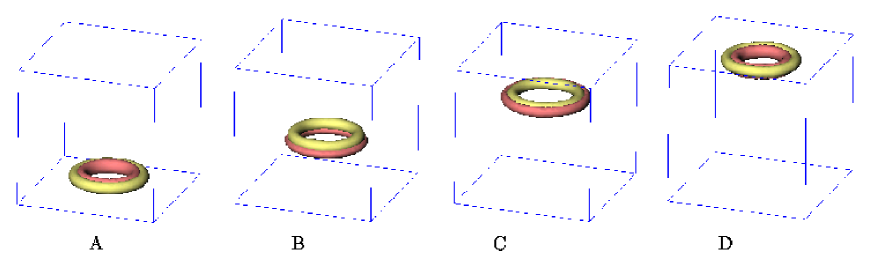
Figure 1: Tubular surfaces indicating the preimages of the points $\mbox{\boldmath$\phi$}=(0,0,-1)$ (light surface) and $\mbox{\boldmath$\phi$}=(-1,0,0)$ (dark surface), at times $t=0,39,78,109,$ for a vortex ring with Hopf charge $Q=0.$

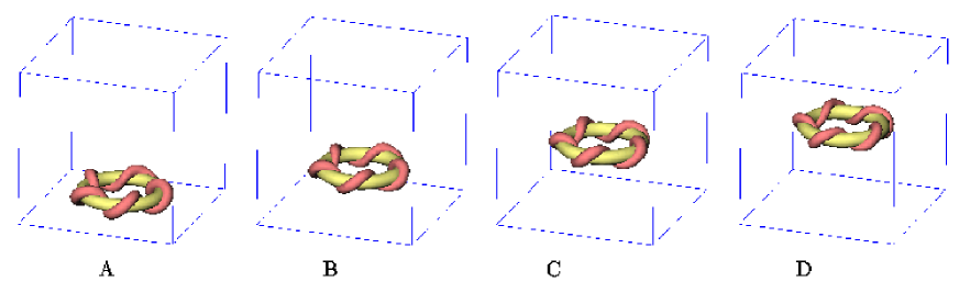
Figure 2: As Figure 1 but with Hopf charge $Q=5.$

Figure 3: The position of the vortex ring as a function of time, for Hopf charge $Q=0$ (upper curve) and $Q=5$ (lower curve).

In Figure 1 the results of a simulation are presented where the initial conditions are as described above with a vortex ring position $z_{0}=-10.$ The results are presented by displaying the location of the vortex ring, which is the curve given by the preimage of the point $\mbox{\boldmath$\phi$}=(0,0,-1).$ To aid visibility this curve is thickened out to a tubular surface (light surface) in Figure 1 by plotting the isosurface $\phi_{3}=0.$ The Hopf charge can be seen by considering the linking number of this curve with the preimage of any other point, which has been chosen to be $\mbox{\boldmath$\phi$}=(-1,0,0),$ and again this is thickened out to a tubular surface (dark surface) in Figure 1 by plotting the isosurface $\phi_{1}=-0.5.$

In Figure 1 the tubular surfaces are displayed at times $t=0,39,78,109.$ A glance at Figure 1A reveals that initially the dark tube is similar to the light tube but has a smaller radius, so the linking number is indeed $Q=0.$ The evolution displayed at later times confirms that the whole configuration drifts upwards, whilst the dark tube rolls around the light tube from the inside to the outside in a periodic motion. This simply reflects the stationary properties of the two-dimensional soliton, where the first two components of the field rotate with an angular frequency $\omega.$ As mentioned above, the profile function given above can be reasonably compared to that of the two-dimensional soliton with $\omega=0.56$ so the expected period of the rolling tube motion is roughly $T\approx 11,$ which is in good agreement with the results of the simulation presented in Figure 1.

In Figure 3 the position of the $Q=0$ vortex ring is shown (upper curve) as a function of time. Note that this is the position in the $x_{3}$ direction, which is along the symmetry axis, and the periodicity of the simulation domain has been taken into account when computing this position. This plot demonstrates that, to a very good approximation, the vortex ring indeed travels with a constant velocity. This velocity is roughly just less than $v\approx 0.2,$ so in the time taken for the vortex ring to move a distance equal to its diameter the two-dimensional soliton forming the vortex ring has made over five revolutions. Thus the translational motion of the vortex ring is somewhat slower than the rotational motion. A careful inspection of the upper curve in Figure 3 reveals that there are very small amplitude wiggles superimposed onto a linear motion. These wiggles correspond to the very slight oscillation in the radius of the vortex ring that results from the fact that the initial conditions are only constructed approximately, and provides evidence for the stability of the vortex ring to axially symmetric perturbations. The simulations presented above were run for a much longer length of time than shown here, so that the vortex ring crosses the periodic boundary of the simulation grid several times, and it continues to propagate at constant speed in the same manner.

Figure 2 displays the results of a simulation identical to the previous one discussed above, except that the initial condition has $Q=5$ rather than $Q=0.$ It is clear to see that the Hopf charge is $Q=5$ because the dark tube winds around the light tube five times. This vortex ring behaves very much like the $Q=0$ vortex ring, except that the propagation speed has been roughly halved to $v\approx 0.1,$ as can be verified from Figure 3 where the lower curve displays the position against time. Performing a number of simulations with different values of the Hopf charge confirms that it is a general feature that increasing only the Hopf charge, while leaving all other parameters unchanged, leads to a reduction in the propagation speed. Note that for a vortex ring with $Q\neq 0$ the internal rotation of the two-dimensional soliton forming the vortex ring is equivalent to a spatial rotation of the whole vortex ring around its symmetry axis, so either interpretation is equally valid, but for $Q=0$ the interpretation as a rotation of the ring around its symmetry axis is not allowed.

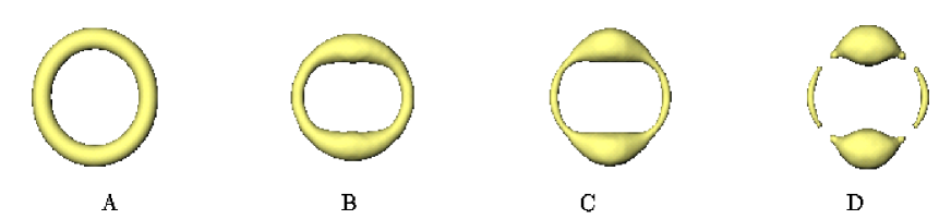
Figure 4: The isosurface $\phi_{3}=0$ at times $t=0,\ 37.5,\ 50,\ 55.625,\$ for a $Q=0$ vortex ring with an initial $10\%$ squashing in the $x_{1}$ direction.

The results presented so far, together with those of Ref.[3], suggest that vortex rings (with sufficient momentum) are stable to axially symmetric perturbations. To investigate the stability properties to general non-axial deformations a rescaling perturbation is applied to the initial conditions to squash the vortex ring by $10\%$ in the $x_{1}$ direction (recall that the symmetry axis is the $x_{3}$ direction). The simulation presented in Figure 4 is on a slightly larger grid containing $151^{3}$ points, but again with $\Delta x=0.25.$ The vortex ring has zero Hopf charge and is a little larger and thicker than in the previous simulations, with the number of spin flips and momentum being $N=2186$ and $P_{3}=5163.$ However, a number of simulations have been performed with various grid sizes and lattice spacings, using vortex rings of varying diameters, thickness and Hopf charge, and all the results are qualitatively similar. The isosurface $\phi_{3}=0,$ which is shown at times $t=0,37.5,50,55.625,$ in Figure 4 illustrates not only the location of the vortex ring but also its thickness, which corresponds to a measure of the local spin flip density in the two-dimensional soliton forming the vortex ring. Clearly there is an instability associated with a migration of spin flips around the vortex ring that leads to a pinching of the vortex ring at certain locations and a compensating fattening at other locations in order to conserve the total number of spin flips. In the simulation presented in Figure 4 the initial squashing perturbation preserves a $C_{2}$ symmetry so the spin flips accumulate at two symmetrical points.

The pinching instability can also be observed in a slightly simpler setting, namely in a straight vortex string, rather than a vortex ring. This provides a reasonable approximation to a segment of the vortex ring if the radius is much larger than the thickness. Numerical simulations on a range of vortex strings with varying thickness and windings, have revealed that all suffer from a pinching instability, and that thicker vortex strings take longer to pinch, but no evidence was found that for a sufficient thickness the instability is removed. For straight vortex strings it would be interesting to confirm this numerically by a study of the negative mode as a function of the string thickness and winding, using a linearized eigenvalue computation. However, it seems unlikely that the instability is lost at a critical thickness, since the unstable mode essentially leads to the formation of magnetic solitons, which in the stationary case are spherically symmetric [5]. It is simple geometry, based on concepts of volume and surface area, that suggests a preference for the spin flips to form lumps rather than tubes.

It is an important observation that the unstable mode associated with the migration of spin flips proceeds towards the formation of magnetic solitons. This is crucial because stationary magnetic solitons exist only for an anisotropic ferromagnet and not in the isotropic limit, as discussed earlier for two-dimensional topological solitons. This suggests that the decay mode might be removed for vortex rings in an isotropic ferromagnet. Although the instability has been discovered using dynamical simulations, it turns out that it can also be studied using a constrained energy minimization method, and this is a slightly better approach since long lived dynamical oscillations do not have to be addressed. This approach is described in the following section, where it is used to investigate the stability of vortex rings in both the anisotropic and isotropic case.

3 Constrained energy minimization

Axially symmetric vortex rings were constructed in Ref.[3] using a constrained energy minimization method. In this section a similar approach is applied but the previous restriction to axially symmetric fields is removed, which enables the investigation of any possible unstable modes.

There is an ansatz which is consistent with the equations of motion and describes a solution that propagates at constant velocity ${\bf v},$ while the first two components of $\phi$ rotate with a frequency $\omega.$ Explicitly, the ansatz reads

$$\phi_{1}+i\phi_{2}=(\widetilde{\phi}_{1}({\bf x}-{\bf v}t)+i\widetilde{\phi}_{2}({\bf x}-{\bf v}t))e^{-i\omega t},\ \ \phi_{3}=\widetilde{\phi}_{3}({\bf x}-{\bf v}t).$$ (3.1)

Substituting this ansatz into the equation of motion (2.2) leads to a partial differential equation for $\mbox{\boldmath$\widetilde{\phi}$}=(\widetilde{\phi}_{1},\widetilde{\phi}_{2},\widetilde{\phi}_{3}).$ This partial differential equation has a variational formulation, which is useful in computing its solutions. Let $\widetilde{E}({\bf P},N)$ be the minimal value of the energy $E,$ given by (2.1), for fixed values of the momentum ${\bf P}$ and number of spin flips $N$. Then the solution of this constrained minimization problem is precisely the function $\widetilde{\phi}$ corresponding to the values [11]

$$\omega=\frac{\partial\widetilde{E}}{\partial N}\bigg{|}_{\bf P},\ \ v_{i}=\frac{\partial\widetilde{E}}{\partial P_{i}}\bigg{|}_{N}.$$ (3.2)

Vortex ring solutions are computed by numerically solving this constrained energy minimization problem using a simulated annealing algorithm with the constraints on $N$ and ${\bf P}$ imposed using a penalty function method. As with the earlier dynamical simulations, the momentum is chosen to point along the $x_{3}$ axis. The energy is discretized using a finite difference method and the grid has the same dimensions as in the dynamical simulations, that is, it contains $151^{3}$ points and has a lattice spacing $\Delta x=0.25.$

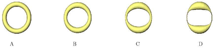
Figure 5: The isosurface $\phi_{3}=0$ during increasing stages of a simulated annealing relaxation of a $Q=1$ vortex ring in the anisotropic system with $A=1.$ The spin flips and momentum are constrained to be $N=2186$ and $P_{3}=5163.$ The initial condition is squashed by $10\%$ in the $x_{1}$ direction and leads to a pinching instability.

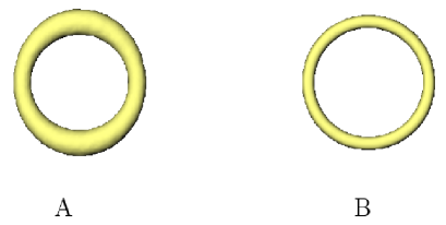
Figure 6: The isosurface $\phi_{3}=0$ during increasing stages of a simulated annealing relaxation of a $Q=1$ vortex ring in the isotropic system ie. $A=0.$ The spin flips and momentum are constrained to be $N=2186$ and $P_{3}=5163.$ The initial condition is a slightly pinched and squashed vortex ring but leads to an axially symmetric stable solution.

Initial conditions can again be created using the axial ansatz (2.8), with an optional squashing in the $x_{1}$ direction to break the axial symmetry. Figure 5 displays the results at increasing stages of a simulated annealing energy relaxation computation, for the system with anisotropy parameter $A=1.$ The initial condition (Figure 5A) is identical to that used in the dynamical simulation presented in Figure 4 except that now $Q=1$ rather than $Q=0.$ The pinching instability is clearly displayed in Figure 5 under constrained energy minimization, and the qualitative features are very similar to those found in the dynamical simulations (compare Figure 4).

Performing similar annealing simulations in the isotropic model ($A=0$) does not produce a pinching instability. As an example, consider the results presented in Figure 6. The initial condition (Figure 6A) is taken from an early stage of the annealing simulation with $A=1$ displayed in Figure 5, and therefore initially has a slight pinching in addition to the squashing. However, with $A=0$ the pinching is reversed and the annealing process results in the stable energy minimizing axially symmetric vortex ring displayed in Figure 6B. There is clearly no pinching instability in the isotropic system. Note that the thickness of the axial vortex ring with $A=0$ appears less than in the $A=1$ system, because of the different localization profiles of solitons in the two systems.

The vortex ring solution of Figure 6B, generated by energy minimization, has been used as an initial condition in a dynamical simulation of the type discussed in section 2, but now in the isotropic system ($A=0$). The results confirm that the vortex ring propagates with an unchanged form at constant speed, in a similar manner to the $A=1$ results. Perturbed vortex rings with broken axial symmetry have also been used as initial conditions in the dynamical simulations and the results confirm the energy minimization computations, in that no pinching instabilities are seen.

4 Conclusion

Propagating vortex ring solutions of the Landau-Lifshitz equation have been presented and their stability properties investigated. It has been shown that for an anisotropic ferromagnet there is a pinching instability which leads to the collapse of the vortex ring, but that this instability disappears for an isotropic ferromagnet. It is possible that even in the anisotropic case there could be parameter values $N,P_{3},Q$ for which vortex rings do not suffer from the pinching instability. By scaling symmetry, the properties of vortex rings for a given $Q$ depend upon the parameter combinations $p=P_{3}/N^{2/3}$ and $a=AN^{2/3}.$ The computations performed in the anisotropic system have been limited to reasonably large values of both $p$ and $a$ (the simulation presented in Figure 5 corresponds to $p\approx 30.7$ and $a\approx 168$). A comprehensive search of parameter space is required to determine if there are any parameter regimes with small $a\neq 0$ that allow stable rings, but this is beyond the scope of the present study. As mentioned earlier, when the anisotropy parameter $A$ is non-zero it can be set to unity, without loss of generality, by rescaling length and time units. However, this means that an investigation of a wide parameter range of $a$ requires substantial variations in $N$ and this is problematic numerically, because a variety of size scales must be accomodated. The alternative is to keep $N$ fixed and vary $A.$ For example, the simulation presented in Figure 5 has been repeated but with $A=0.1$ rather than $A=1$, corresponding to a less anisotropic regime with $a\approx 16.8$. The pinching instabilty is again revealed, but on a time scale that is an order of magnitude larger than in the previous case. It is therefore difficult to determine whether the instability is removed for a small but non-zero value of $a,$ or only in the limit $a=0.$ In either case, if the anisotropy is small, then any potential pinching instability will only develop on large timescales and therefore may not be important, since the lifetime of any excitation will be limited by dissipation, which has been neglected here. These results suggests that any future attempts at an experimental observation of vortex rings will most likely succeed in ferromagnets where the anisotropy is as weak as possible.

In a different system to the one studied here (though it is related and has the same field content) stable static Hopf solitons exist which form knotted configurations [1, 10]. It would be very interesting if similar propagating knotted Hopf solitons existed in ferromagnets, thereby providing a physical system in which knots may be observed experimentally. Clearly the anisotropic system is unlikely to support such solitons due to the pinching instability, but there is a possibility that the isotropic system might. A variety of knotted and linked vortex string field configurations with various Hopf charges can be generated using an ansatz involving rational maps [10]. Such fields have been used as initial conditions in the constrained energy minimization method discussed in the previous section, but unfortunately this has, as yet, not produced any stable knotted or linked solutions. The relevant obstacle appears to be the fact that to minimize energy with a constrained momentum it is favourable to localize the field close to a plane which is perpendicular to the momentum; as in vortex rings. As a result, initially knotted fields relax by flattening and this leads to vortex string reconnections and ultimately the formation of vortex rings.

In addition to the conserved quantities of spin flips $N$ and momentum ${\bf P}$ there is also a conserved angular momentum ${\bf L}$ [8]. For axially symmetric vortex rings the angular momentum points along the symmetry axis and has the value $L_{3}=QN,$ which reflects the fact mentioned earlier that for a vortex ring with $Q\neq 0$ the internal rotation of the two-dimensional soliton forming the vortex ring is equivalent to a spatial rotation of the whole vortex ring around its symmetry axis. To prevent knotted initial configurations from relaxing to axially symmetric vortex rings a constraint on $L_{3}$ can be imposed with $L_{3}\neq QN.$ However, the result of such relaxations simply tends to produce vortex rings which are elliptical rather than circular. In summary, the current evidence suggests that stable propagating knotted vortex strings appear unlikely to exist, though it remains an open problem as there are a large range of parameter values for $N,{\bf P},{\bf L},Q$ and only a handful of specific examples have currently been investigated.

Finally, it is interesting to note that there is a comparison to be made between vortex rings in ferromagnets and similar objects in relativistic field theories. Non-topological straight string solitons carrying Noether charge suffer from a similar pinching instability [4], with a migration of charge along the string leading to the conversion of the string into non-topological solitons. Vortons, which arise in cosmological applications, are closed loops of superconducting cosmic strings carrying both current and charge. They have a number of similarities with the vortex rings studied here, and in particular there are parameter regimes in which a related pinching instability exists [6]. Thus vortex rings in ferromagnets may be yet another example in which analogues of cosmological phenomena may be studied in condensed matter systems in the laboratory.

References

- [1] R. A. Battye and P. M. Sutcliffe, Knots as stable soliton solutions in a three-dimensional classical field theory, Phys. Rev. Lett. 81, 4798 (1998); Solitons, links and knots, Proc. R. Soc. Lond. A455, 4305 (1999).
- [2] A. A. Belavin and A. M. Polyakov, Metastable states of two-dimensional isotropic ferromagnets, JETP Lett. 22, 245 (1975).
- [3] N. R. Cooper, Propagating magnetic vortex rings in ferromagnets, Phys. Rev. Lett. 82, 1554 (1999).
- [4] E. Copeland, E. W. Kolb and K. Lee, Existence and stability of nontopological strings, Phys. Rev. D38, 3023 (1988).
- [5] A. M. Kosevich, B. A. Ivanov and A. S. Kovalev, Magnetic solitons, Phys. Rep. 194, 117 (1990).
- [6] Y. Lemperiere and E. P. S. Shellard, On the behaviour and stability of superconducting currents, Nucl. Phys. B649, 511 (2003); Vorton existence and stability, Phys. Rev. Lett. 91, 141601 (2003).
- [7] N. Papanicolaou, Dynamics of magnetic vortex rings, NATO ASI Series C403, 151 (1993).
- [8] N. Papanicolaou and T. N. Tomaras, Dynamics of magnetic vortices, Nucl. Phys. B360, 425 (1991).
- [9] B. Piette and W. J. Zakrzewski, Localized solutions in a 2 dimensional Landau-Lifshitz model, Physica D119, 314 (1998).
- [10] P. M. Sutcliffe, Knots in the Skyrme-Faddeev model, arXiv:0705.1468 (2007).
- [11] J. Tjon and J. Wright, Solitons in the continuous Heisenberg spin chain, Phys. Rev. B15, 3470 (1977).