Surfaces from Circles

Abstract

In the search for appropriate discretizations of surface theory it is crucial to preserve such fundamental properties of surfaces as their invariance with respect to transformation groups. We discuss discretizations based on Möbius invariant building blocks such as circles and spheres. Concrete problems considered in these lectures include the Willmore energy as well as conformal and curvature line parametrizations of surfaces. In particular we discuss geometric properties of a recently found discrete Willmore energy. The convergence to the smooth Willmore functional is shown for special refinements of triangulations originating from a curvature line parametrization of a surface. Further we treat special classes of discrete surfaces such as isothermic and minimal. The construction of these surfaces is based on the theory of circle patterns, in particular on their variational description.

1 Why from Circles?

The theory of polyhedral surfaces aims to develop discrete equivalents of the geometric notions and methods of smooth surface theory. The latter appears then as a limit of refinements of the discretization. Current interest in this field derives not only from its importance in pure mathematics but also from its relevance for other fields like computer graphics.

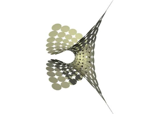
Figure 1: Discrete surfaces made from circles: general simplicial surface and a discrete minimal Enneper surface.

One may suggest many different reasonable discretizations with the same smooth limit. Which one is the best? In the search for appropriate discretizations, it is crucial to preserve the fundamental properties of surfaces. A natural mathematical discretization principle is the invariance with respect to transformation groups. A trivial example of this principle is the invariance of the theory with respect to Euclidean motions. A less trivial but well-known example is the discrete analog for the local Gaussian curvature defined as the angle defect $G(v)=2\pi-\sum\alpha_{i},$ at a vertex $v$ of a polyhedral surface. Here the $\alpha_{i}$ are the angles of all polygonal faces (see Fig. 3) of the surface at vertex $v$. The discrete Gaussian curvature $G(v)$ defined in this way is preserved under isometries, which is a discrete version of the theoremum egregium of Gauss.

In these lectures, we focus on surface geometries invariant under Möbius transformations. Recall that Möbius transformations form a finite-dimensional Lie group generated by inversions in spheres (see Fig. 2).

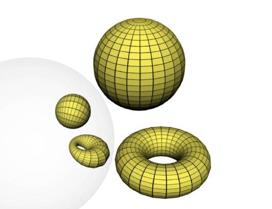
Figure 2: Inversion $B\mapsto C$ in a sphere, $\mid AB\mid\mid AC\mid=R^{2}$. A sphere and a torus of revolution and their inversions in a sphere: spheres are mapped to spheres.

Möbius transformations can be also thought as compositions of translations, rotations, homotheties and inversions in spheres. Alternatively, in dimensions $n\geq 3$ Möbius transformations can be characterized as conformal transformations: Due to Liouville’s theorem any conformal mapping $F:U\to V$ between two open subsets $U,V\subset{\mathbb{R}}^{n},n\geq 3$ is a Möbius transformation.

Many important geometric notions and properties are known to be preserved by Möbius transformations. The list includes in particular:

• spheres of any dimension, in particular circles (planes and straight lines are treated as infinite spheres and circles),

• intersection angles between spheres (and circles),

• curvature line parametrization,

• conformal parametrization,

• isothermic parametrization ( conformal curvature line parametrization),

• the Willmore functional (see Section 2).

For discretization of Möbius-invariant notions it is natural to use Möbius-invariant building blocks. This observation leads us to the conclusion that the discrete conformal or curvature line parametrizations of surfaces and the discrete Willmore functional should be formulated in terms of circles and spheres.

2 Discrete Willmore Energy

The Willmore functional [39] for a smooth surface $\mathcal{S}$ in 3-dimensional Euclidean space is

$${\mathcal{W}(S)}=\frac{1}{4}\int_{\mathcal{S}}(k_{1}-k_{2})^{2}dA=\int_{\mathcal{S}}H^{2}dA-\int_{\mathcal{S}}KdA.$$

Here $dA$ is the area element, $k_{1}$ and $k_{2}$ the principal curvatures, $H=\frac{1}{2}(k_{1}+k_{2})$ the mean curvature, and $K=k_{1}k_{2}$ the Gaussian curvature of the surface.

Let us mention two important properties of the Willmore energy:

• ${\mathcal{W}(S)}\geq 0$ and ${\mathcal{W}(S)}=0$ if and only if $\mathcal{S}$ is a round sphere.

• $\mathcal{W}(S)$ (and the integrand $(k_{1}-k_{2})^{2}dA$) is Möbius invariant [1, 39]

Whereas the first claim almost immediately follows from the definition, the second is a non-trivial property. Observe that for closed surfaces $\mathcal{W}(S)$ and $\int_{\mathcal{S}}H^{2}dA$ differ by a topological invariant $\int KdA=2\pi\chi(S)$. We prefer the definition of $\mathcal{W}(S)$ with a Möbius invariant integrand.

Observe that minimization of the Willmore energy $\mathcal{W}$ seeks to make the surface “as round as possible”. This property and the Möbius invariance are two principal points of the geometric discretization of the Willmore energy suggested in [3]. In this section we present the main results of [3] with complete derivations, some of which were omitted there.

2.1 Discrete Willmore functional for simplicial surfaces

Let $S$ be a simplicial surface in 3-dimensional Euclidean space with vertex set $V$, edges $E$ and (triangular) faces $F$. We define the discrete Willmore energy of $S$ using the circumcircles of its faces. Each (internal) edge $e\in E$ is incident to two triangles. A consistent orientation of the triangles naturally induces an orientation of the corresponding circumcircles. Let $\beta(e)$ be the external intersection angle of the circumcircles of the triangles sharing $e$, meaning the angle between the tangent vectors of the oriented circumcircles (at either intersection point).

Definition 2.1.

The local discrete Willmore energy at a vertex $v$ is the sum

$$W(v)=\sum_{e\ni v}\beta(e)-2\pi.$$

over all edges incident to $v$. The discrete Willmore energy of a compact simplicial surface $S$ without boundary is the sum over all vertices

$$W(S)=\dfrac{1}{2}\sum_{v\in V}W(v)=\sum_{e\in E}\beta(e)-\pi\mid V\mid.$$

Here $|V|$ is the number of vertices of $S$.

Figure 3: Definition of discrete Willmore energy

Figure 3 presents two neighboring circles with their external intersection angle $\beta_{i}$ as well as a view “from the top” at a vertex $v$ showing all $n$ circumcircles passing through $v$ with the corresponding intersection angles $\beta_{1},\ldots,\beta_{n}$. For simplicity we will consider only simplicial surfaces without boundary.

The energy $W(S)$ is obviously invariant with respect to Möbius transformations.

The star $S(v)$ of the vertex $v$ is the subcomplex of $S$ consisting of the triangles incident with $v$. The vertices of $S(v)$ are $v$ and all its neighbors. We call $S(v)$ convex if for each of its faces $f\in F(S(v))$ the star $S(v)$ lies to one side of the plane of $f$ and strictly convex if the intersection of $S(v)$ with the plane of $f$ is $f$ itself.

Proposition 2.2.

The conformal energy is nonnegative

$$W(v)\geq 0,$$

and vanishes if and only if the star $S(v)$ is convex and all its vertices lie on a common sphere.

The proof of this proposition is based on an elementary lemma.

Lemma 2.3.

Let $\mathcal{P}$ be a (not necessarily planar) $n$-gon with external angles $\beta_{i}$. Choose a point $P$ and connect it to all vertices of $\mathcal{P}$. Let $\alpha_{i}$ be the angles of the triangles at the tip $P$ of the pyramid thus obtained (see Figure 4). Then

$$\sum_{i=1}^{n}\beta_{i}\geq\sum_{i=1}^{n}\alpha_{i},$$

and equality holds if and only if $\mathcal{P}$ is planar and convex and the vertex $P$ lies inside $\mathcal{P}$.

Figure 4: Proof of Lemma 2.3

Proof.

Denote by $\gamma_{i}$ and $\delta_{i}$ the angles of the triangles at the vertices of $\mathcal{P}$, as in Figure 4. The claim of Lemma 2.3 follows from adding over all $i=1,\ldots,n$ the two obvious relations

$$\beta_{i+1} \geq \pi-(\gamma_{i+1}+\delta_{i})$$

$$\alpha_{i} = \pi-(\gamma_{i}+\delta_{i}).$$

All inequalities become equalities only in the case when $\mathcal{P}$ is planar, convex and contains $P$. ∎

For $P$ in the convex hull of $\mathcal{P}$ we have $\sum\alpha_{i}\geq 2\pi$. As a corollary we obtain a polygonal version of Fenchel’s theorem [18]:

Corollary 2.4.

$$\sum_{i=1}^{n}\beta_{i}\geq 2\pi.$$

Proof of Proposition 2.2. The claim of Proposition 2.2 is invariant with respect to Möbius transformations. Applying a Möbius transformation $M$ that maps the vertex $v$ to infinity, $M(v)=\infty$, we make all circles passing through $v$ into straight lines and arrive at the geometry shown in Figure 4 with $P=M(\infty)$. Now the result follows immediately from Corollary 2.4.

Theorem 2.5.

Let $S$ be a compact simplicial surface without boundary. Then

$$W(S)\geq 0,$$

and equality holds if and only if $S$ is a convex polyhedron inscribed in a sphere, i.e. a Delaunay triangulation of a sphere.

Proof.

Only the second statement needs to be proven. By Proposition 2.2, the equality $W(S)=0$ implies that the star of each vertex of $S$ is convex (but not necessarily strictly convex). Deleting the edges that separate triangles lying in a common plane, one obtains a polyhedral surface $S_{P}$ with circular faces and all strictly convex vertices and edges. Proposition 2.2 implies that for every vertex $v$ there exists a sphere $S_{v}$ with all vertices of the star $S(v)$ lying on it. For any edge $(v_{1},v_{2})$ of $S_{P}$ two neighboring spheres $S_{v_{1}}$ and $S_{v_{2}}$ share two different circles of their common faces. This implies $S_{v_{1}}=S_{v_{2}}$ and finally the coincidence of all the spheres $S_{v}$. ∎

2.2 Noninscribable polyhedra

The minimization of the conformal energy for simplicial spheres is related to a classical result of Steinitz [37], who showed that there exist abstract simplicial 3-polytopes without geometric realizations as convex polytopes with all vertices on a common sphere. We call these combinatorial types noninscribable.

Let $S$ be a simplicial sphere with vertices colored in black and white. Denote the sets of white and black vertices by $V_{w}$ and $V_{b}$ respectively, $V=V_{w}\cup V_{b}$. Assume that there are no edges connecting two white vertices and denote the sets of the edges connecting white and black vertices and two black vertices by $E_{wb}$ and $E_{bb}$ respectively, $E=E_{wb}\cup E_{bb}$. The sum of the local discrete Willmore energies over all white vertices can be represented as

$$\sum_{v\in V_{w}}W(v)=\sum_{e\in E_{wb}}\beta(e)-2\pi|V_{w}|.$$

Its nonnegativity yields $\sum_{e\in E_{wb}}\beta(e)\geq 2\pi|V_{w}|$. For the discrete Willmore energy of $S$ this implies

$$W(S)=\sum_{e\in E_{wb}}\beta(e)+\sum_{e\in E_{bb}}\beta(e)-\pi(|V_{w}|+|V_{b}|)\geq\pi(|V_{w}|-|V_{b}|).$$ (2.1)

The equality here holds if and only if $\beta(e)=0$ for all $e\in E_{bb}$ and the star of any white vertices is convex, with vertices lying on a common sphere. We come to the conclusion that the polyhedra of this combinatorial type with $|V_{w}|>|V_{b}|$ have positive Willmore energy and thus cannot be realized as convex polyhedra all of whose vertices belong to a sphere. These are exactly the noninscribable examples of Steinitz [21].

One such example is presented in Figure 5. Here the centers of the edges of the tetrahedron are black and all other vertices are white, so $|V_{w}|=8,|V_{b}|=6$. The estimate (2.1) implies that the discrete Willmore energy of any polyhedron of this type is at least $2\pi$. The polyhedra with energy equal to $2\pi$ are constructed as follows. Take a tetrahedron, color its vertices white and chose one black vertex per edge. Draw circles through each white vertex and its two black neighbors. We get three circles on each face. Due to Miquel’s theorem (see Fig. 10) these three circles intersect at one point. Color this new vertex white. Connect it by edges to all black vertices of the triangle and connect pairwise the black vertices of the original faces of the tetrahedron. The constructed polyhedron has $W=2\pi$.

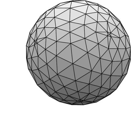
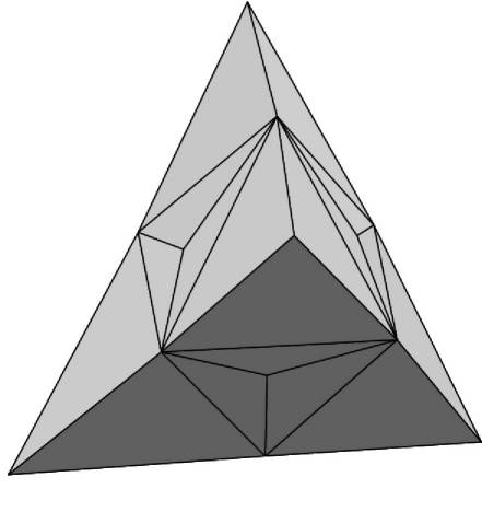
Figure 5: Discrete Willmore spheres of inscribable ($W=0$) and non-inscribable ($W>0$) types.

To construct further polyhedra with $|V_{w}|>|V_{b}|$, take a polyhedron $\hat{P}$ whose number of faces is greater then the number of vertices $|\hat{F}|>|\hat{V}|$. Color all the vertices black, add white vertices at the faces and connect them to all black vertices of a face. This yields a polyhedron with $|V_{w}|=|\hat{F}|>|V_{b}|=|\hat{V}|$. Hodgson, Rivin and Smith [24] have found a characterization of inscribable combinatorial types, based on a transfer to the Klein model of hyperbolic 3-space. Their method is related to the methods of construction of discrete minimal surfaces in Section 5.

The example in Figure 5 (right) is one of the few for which the minimum of the discrete Willmore energy can be found by elementary methods. Generally this is a very appealing (but probably difficult) problem of discrete differential geometry (see the discussion in [3]).

Complete understanding of noninscribable simplicial spheres is an interesting mathematical problem. However the phenomenon of existence of such spheres might be seen as a problem in using of the discrete Willmore functional for applications in computer graphics, such as the fairing of surfaces. Fortunately the problem disappears after just one refinement step: all simplicial spheres become inscribable. Let $\bf S$ be an abstract simplicial sphere. Define its refinement $\bf S_{R}$ as follows: split every edge of $\bf S$ in two by inserting additional vertices, and connect these new vertices sharing a face of $\bf S$ by additional edges ($1\to 4$ refinement, see Figure 7 (left)).

Proposition 2.6.

The refined simplicial sphere $\bf S_{R}$ is inscribable, and thus there exists a polyhedron $S_{R}$ with the combinatorics of $\bf S_{R}$ and $W(S_{R})=0$.

Proof.

Koebe’s theorem (see Theorem 5.3, Section 5) states that every abstract simplicial sphere $\bf S$ can be realized as a convex polyhedron $S$ all of whose edges touch a common sphere $S^{2}$. Starting with this realization $S$ it is easy to construct a geometric realization $S_{R}$ of the refinement $\bf S_{R}$ inscribed in $S^{2}$. Indeed, choose the touching points of the edges of $S$ with $S^{2}$ as the additional vertices of $S_{R}$ and project the original vertices of $S$ (which lie outside of the sphere $S^{2}$) to $S^{2}$. One obtains a convex simplicial polyhedron $S_{R}$ inscribed in $S^{2}$. ∎

2.3 Computation of the energy

For derivation of some formulas it will be convenient to use the language of quaternions. Let $\{{\bf 1},{\bf i},{\bf j},{\bf k}\}$ be the standard basis

$${\bf ij}={\bf k},\quad{\bf ij}={\bf k},\quad{\bf ij}={\bf k},\quad{\bf ii}={\bf jj}={\bf kk}=-{\bf 1}$$

of the quaternion algebra ${\mathbb{H}}$. A quaternion $q=q_{0}{\bf 1}+q_{1}{\bf i}+q_{2}{\bf j}+q_{3}{\bf k}$ is decomposed in its real part ${\rm Re}\ q:=q_{0}\in{\mathbb{R}}$ and imaginary part ${\rm Im}\ q:=q_{1}{\bf i}+q_{2}{\bf j}+q_{3}{\bf k}\in{\rm Im}\ {\mathbb{H}}$. The absolute value of $q$ is $|q|:=q_{0}^{2}+q_{1}^{2}+q_{2}^{2}+q_{3}^{2}$.

We identify vectors in ${\mathbb{R}}^{3}$ with imaginary quaternions

$$v=(v_{1},v_{2},v_{3})\in{\mathbb{R}}^{3}\quad\longleftrightarrow\quad v=v_{1}{\bf i}+v_{2}{\bf j}+v_{3}{\bf k}\in{\rm Im}\ {\mathbb{H}}$$

and do not distinguish them in our notation. For the quaternionic product this implies

$$vw=-\langle v,w\rangle+v\times w,$$ (2.2)

where $\langle v,w\rangle$ and $v\times w$ are the scalar and vector products in ${\mathbb{R}}^{3}$.

Definition 2.7.

Let $x_{1},x_{2},x_{3},x_{4}\in{\mathbb{R}}^{3}\cong{\rm Im}\ {\mathbb{H}}$ be points in 3-dimensional Euclidean space. The quaternion

$$q(x_{1},x_{2},x_{3},x_{4}):=(x_{1}-x_{2})(x_{2}-x_{3})^{-1}(x_{3}-x_{4})(x_{4}-x_{1})^{-1}$$

is called the cross-ratio of $x_{1},x_{2},x_{3},x_{4}$.

The cross-ratio is quite useful due to its Möbius properties:

Lemma 2.8.

The absolute value and real part of the cross-ratio $q(x_{1},x_{2},x_{3},x_{4})$ (or equivalently $|q|$ and $|{\rm Im}\ q|$) are preserved by Möbius transformations. The quadrilateral $x_{1},x_{2},x_{3},x_{4}$ is circular if and only if $q(x_{1},x_{2},x_{3},x_{4})\in{\mathbb{R}}$.

Consider two triangles with a common edge. Let $a,b,c,d\in{{\mathbb{R}}^{3}}$ be their other edges, oriented as in Fig.6.

Figure 6: Formula for the angle between circumcircles

Proposition 2.9.

The external angle $\beta\in[0,\pi]$ between the circumcircles of the triangles in Figure 6 is given by any of the equivalent formulas:

$$\cos(\beta) = -\dfrac{{\rm Re}\ q}{\mid q\mid}=-\dfrac{{\rm Re}\ (abcd)}{\mid abcd\mid}=$$ (2.3)

$$= \dfrac{\langle a,c\rangle\langle b,d\rangle-\langle a,b\rangle\langle c,d\rangle-\langle b,c\rangle\langle d,a\rangle}{\mid a\mid\mid b\mid\mid c\mid\mid d\mid}.$$

Here $q=ab^{-1}cd^{-1}$ is the cross-ratio of the quadrilateral.

Proof.

Since ${\rm Re}\ q$, $|q|$ and $\beta$ are Möbius-invariant, it is enough to prove the first formula for the planar case $a,b,c,d\in{\mathbb{C}}$, mapping all four vertices to a plane by a Möbius transformation. In this case $q$ becomes the classical complex cross-ratio. Considering the arguments $a,b,c,d\in{\mathbb{C}}$ one easily arrives at $\beta=\pi-\arg q$. The second representation follows from the identity $b^{-1}=-b/|b|$ for imaginary quaternions. Finally applying (2.2) we obtain

$${\rm Re}\ (abcd)=\langle a,b\rangle\langle c,d\rangle-\langle a\times b,c\times d\rangle=$$

$$\langle a,b\rangle\langle c,d\rangle+\langle b,c\rangle\langle d,a\rangle-\langle a,c\rangle\langle b,d\rangle.$$

∎

2.4 Smooth limit

The discrete energy $W$ is not only a discrete analogue of the Willmore energy. In this section we show that it approximates the smooth Willmore energy, although the smooth limit is very sensitive to the refinement method and should be chosen in a special way. We consider a special infinitesimal triangulation which can be obtained in the limit of $1\to 4$ refinements (see Fig. 7 (left)) of a triangulation of a smooth surface. Intuitively it is clear that in the limit one has a regular triangulation such that almost every vertex is of valence 6 and neighboring triangles are congruent up to sufficiently high order of $\epsilon$ ($\epsilon$ is the order of the distances between neighboring vertices).

Figure 7: Smooth limit of the discrete Willmore energy. Left: The $1\to 4$ refinement. Middle: An infinitesimal hexagon in the parameter plane with a (horizontal) curvature line. Right: The $\beta$-angle corresponding to two neighboring triangles in ${\mathbb{R}}^{3}$.

We start with a comparison of the discrete and smooth Willmore energies for an important modelling example. Consider a neighborhood of a vertex $v\in{\mathcal{S}}$, and represent the smooth surface locally as a graph over the tangent plane at $v$:

$${\mathbb{R}}^{2}\ni(x,y)\mapsto f(x,y)=\Big{(}x,y,{1\over 2}(k_{1}x^{2}+k_{2}y^{2})+o(x^{2}+y^{2})\Big{)}\in{\mathbb{R}}^{3},\quad(x,y)\to 0.$$

Here $x,y$ are the curvature directions and $k_{1},k_{2}$ are the principal curvatures at $v$. Let the vertices $(0,0),a=(a_{1},a_{2})$ and $b=(b_{1},b_{2})$ in the parameter plane form an acute triangle. Consider the infinitesimal hexagon with vertices $\epsilon a,\epsilon b,\epsilon c,-\epsilon a,-\epsilon b,-\epsilon c$, (see Figure 7 (middle)), with $b=a+c$. The coordinates of the corresponding points on the smooth surface are

$$f(\pm\epsilon a) = \epsilon(\pm a_{1},\pm a_{2},\epsilon r_{a}+o(\epsilon)),$$

$$f(\pm\epsilon c) = \epsilon(\pm c_{1},\pm c_{2},\epsilon r_{c}+o(\epsilon)),$$

$$f(\pm\epsilon b) = (f(\pm\epsilon a)+f(\pm\epsilon c))+\epsilon^{2}R,\quad R=(0,0,r+o(\epsilon)),$$

where

$$r_{a}={1\over 2}(k_{1}a_{1}^{2}+k_{2}a_{2}^{2}),\quad r_{c}={1\over 2}(k_{1}c_{1}^{2}+k_{2}c_{2}^{2}),\quad r=(k_{1}a_{1}c_{1}+k_{2}a_{2}c_{2})$$

and $a=(a_{1},a_{2}),c=(c_{1},c_{2})$.

We will compare the discrete Willmore energy $W$ of the simplicial surface comprised by the vertices $f(\epsilon a),\ldots,f(-\epsilon c)$ of the hexagonal star with the classical Willmore energy ${\mathcal{W}}$ of the corresponding part of the smooth surface $\mathcal{S}$. Some computations are required for this. Denote by $\epsilon A=f(\epsilon a),\epsilon B=f(\epsilon b),\epsilon C=f(\epsilon c)$ the vertices of two corresponding triangles (as in Figure 7 (right)), and also by $|a|$ the length of $a$ and by $\langle a,c\rangle=a_{1}c_{1}+a_{2}c_{2}$ the corresponding scalar product.

Lemma 2.10.

The external angle $\beta(\epsilon)$ between the circumcircles of the triangles with the vertices $(0,A,B)$ and $(0,B,C)$ (as in Figure 7 (right)) is given by

$$\beta(\epsilon)=\beta(0)+w(b)+o(\epsilon^{2}),\quad\epsilon\to 0,\quad w(b)=\epsilon^{2}\dfrac{g\cos\beta(0)-h}{|a|^{2}|c|^{2}\sin\beta(0)}.$$ (2.4)

Here $\beta(0)$ is the external angle of the circumcircles of the triangles $(0,a,b)$ and $(0,b,c)$ in the plane, and

$$g = |a|^{2}r_{c}(r+r_{c})+|c|^{2}r_{a}(r+r_{a})+{r^{2}\over 2}(|a|^{2}+|c|^{2}),$$

$$h = |a|^{2}r_{c}(r+r_{c})+|c|^{2}r_{a}(r+r_{a})-\langle a,c\rangle(r+2r_{a})(r+2r_{c}).$$

Proof.

Formula (2.3) with $a=-C,b=A,c=C+\epsilon R,d=-A-\epsilon R$ yields

$$\cos\beta=\dfrac{\langle C,C+\epsilon R\rangle\langle A,A+\epsilon R\rangle-\langle A,C\rangle\langle A+\epsilon R,C+\epsilon R\rangle-\langle A,C+\epsilon R\rangle\langle A+\epsilon R,C\rangle}{|A||C||A+\epsilon R||C+\epsilon R|},$$

where $|A|$ is the length of $A$. Substituting the expressions for $A,C,R$ we see that the term of order $\epsilon$ of the numerator vanishes, and we obtain for the numerator

$$|a|^{2}|c|^{2}-2\langle a,c\rangle^{2}+\epsilon^{2}h+o(\epsilon^{2}).$$

For the terms in the denominator we get

$$|A|=|a|\left(1+{r_{a}^{2}\over 2|a|^{2}}\epsilon^{2}+o(\epsilon^{2})\right),\quad|A+\epsilon R|=|a|\left(1+{(r+r_{a})^{2}\over 2|a|^{2}}\epsilon^{2}+o(\epsilon^{2})\right)$$

and similar expression for $|C|$ and $|C+\epsilon R|$. Substituting this to the formula for $\cos\beta$ we obtain

$$\cos\beta=1-2\left(\dfrac{\langle a,c\rangle}{|a||c|}\right)^{2}+\dfrac{\epsilon^{2}}{|a|^{2}|c|^{2}}\left(h-g(1-2\left(\dfrac{\langle a,c\rangle}{|a||c|}\right)^{2})\right)+o(\epsilon^{2}).$$

Observe that this formula can be read as

$$\cos\beta(\epsilon)=\cos\beta(0)+\dfrac{\epsilon^{2}}{|a|^{2}|c|^{2}}\left(h-g\cos\beta(0)\right)+o(\epsilon^{2}),$$

which implies the asymptotic (2.4). ∎

The term $w(b)$ is in fact the part of the discrete Willmore energy of the vertex $v$ coming from the edge $b$. Indeed the sum of the angles $\beta(0)$ over all 6 edges meeting at $v$ is $2\pi$. Denote by $w(a)$ and $w(c)$ the parts of the discrete Willmore energy corresponding to the edges $a$ and $c$. Observe that for the opposite edges (for example $a$ and $-a$) the terms $w$ coincide. Denote $W_{\epsilon}(v)$ the discrete Willmore energy of the simplicial hexagon we consider. We have

$$W_{\epsilon}(v)=(w(a)+w(b)+w(c))+o(\epsilon^{2}).$$

On the other hand the part of the classical Willmore functional corresponding to the vertex $v$ is

$${\mathcal{W}}_{\epsilon}(v)={1\over 4}(k_{1}-k_{2})^{2}S+0(\epsilon^{2}),$$

where the area $S$ is one third of the area of the hexagon or, equivalently, twice the area of one of the triangles in the parameter domain

$$S=\epsilon^{2}|a||c|\sin\gamma.$$

Here $\gamma$ is the angle between the vectors $a$ and $c$. An elementary geometric consideration implies

$$\beta(0)=2\gamma-\pi.$$ (2.5)

We are interested in the quotient $W_{\epsilon}/{\mathcal{W}}_{\epsilon}$ which is obviously scale invariant. Let us normalize $|a|=1$ and parametrize the triangles by the angles between the edges and by the angle to the curvature line (see Fig. 7 (middle)).

$$(a_{1},a_{2}) = (\cos\phi_{1},\sin\phi_{1}),$$ (2.6)

$$(c_{1},c_{2}) = (\dfrac{\sin\phi_{2}}{\sin\phi_{3}}\cos(\phi_{1}+\phi_{2}+\phi_{3}),\dfrac{\sin\phi_{2}}{\sin\phi_{3}}\sin(\phi_{1}+\phi_{2}+\phi_{3})).$$

The moduli space of the regular lattices of acute triangles is described as follows

$$\Phi=\{\phi=(\phi_{1},\phi_{2},\phi_{3})\in{\mathbb{R}}^{3}|0\leq\phi_{1}<{\pi\over 2},\ 0<\phi_{2}<{\pi\over 2},\ 0<\phi_{3}<{\pi\over 2},\ {\pi\over 2}<\phi_{2}+\phi_{3}\}.$$

Proposition 2.11.

The limit of the quotient of the discrete and smooth Willmore energies

$$Q(\phi):=\lim_{\epsilon\to 0}\dfrac{W_{\epsilon}(v)}{{\mathcal{W}}_{\epsilon}(v)}$$

is independent of the curvatures of the surface and depends on the geometry of the triangulation only. It is

$$Q(\phi)=1-\dfrac{(\cos 2\phi_{1}\cos\phi_{3}+\cos(2\phi_{1}+2\phi_{2}+\phi_{3}))^{2}+(\sin 2\phi_{1}\cos\phi_{3})^{2}}{4\cos\phi_{2}\cos\phi_{3}\cos(\phi_{2}+\phi_{3})},$$ (2.7)

and we have $Q>1$. The infimum $\inf_{\Phi}Q(\phi)=1$ corresponds to one the cases when two of the three lattice vectors $a,b,c$ are in the principal curvature directions

• $\phi_{1}=0,\phi_{2}+\phi_{3}\to{\pi\over 2}$,

• $\phi_{1}=0,\phi_{2}\to{\pi\over 2}$,

• $\phi_{1}+\phi_{2}={\pi\over 2},\phi_{3}\to{\pi\over 2}$.

Proof.

is based on a direct but rather involved computation. We have used the Mathematica computer algebra system for some of the computations. Introduce

$$\tilde{w}:={4w\over(k_{1}-k_{2})^{2}S}.$$

This gives in particular

$$\tilde{w}(b)=2\dfrac{h+g(2\cos^{2}\gamma-1)}{(k_{1}-k_{2})^{2}|a|^{3}|c|^{3}\cos\gamma\sin^{2}\gamma}=2\dfrac{h+g(2{\langle a,c\rangle^{2}\over|a|^{2}|c|^{2}}-1)}{(k_{1}-k_{2})^{2}\langle a,c\rangle(|a|^{2}|c|^{2}-\langle a,c\rangle^{2})}.$$

Here we have used the relation (2.5) between $\beta(0)$ and $\gamma$. In the sum over the edges $Q=\tilde{w}(a)+\tilde{w}(b)+\tilde{w}(c)$ the curvatures $k_{1},k_{2}$ disappear and we get $Q$ in terms of the coordinates of $a$ and $c$:

$$Q = 2((a_{1}^{2}c_{2}^{2}+a_{2}^{2}c_{1}^{2})(a_{1}c_{1}+a_{2}c_{2})+a_{1}^{2}c_{1}^{2}(a_{2}^{2}+c_{2}^{2})+a_{2}^{2}c_{2}^{2}(a_{1}^{2}+c_{1}^{2})+$$

$$2a_{1}a_{2}c_{1}c_{2}((a_{1}+c_{1})^{2}+(a_{2}+c_{2})^{2}))/$$

$$\left((a_{1}c_{1}+a_{2}c_{2})(a_{1}(a_{1}+c_{1})+a_{2}(a_{2}+c_{2}))((a_{1}+c_{1})c_{1}+(a_{2}+c_{2})c_{2})\right).$$

Substituting the angle representation (2.6) we obtain

$$Q=\dfrac{\sin 2\phi_{1}\sin 2(\phi_{1}+\phi_{2})+2\cos\phi_{2}\sin(2\phi_{1}+\phi_{2})\sin 2(\phi_{1}+\phi_{2}+\phi_{3})}{4\cos\phi_{2}\cos\phi_{3}\cos(\phi_{2}+\phi_{3})}.$$

One can check that this formula is equivalent to (2.7). Since the denominator in (2.7) on the space $\Phi$ is always negative we have $Q>1$. The identity $Q=1$ holds only if both terms in the nominator of (2.7) vanish. This leads exactly to the cases indicated in the proposition when the lattice vectors are directed along the curvature lines. Indeed the vanishing of the second term in the nominator implies either $\phi_{1}=0$ or $\phi_{3}\to{\pi\over 2}$. Vanishing of the first term in the nominator with $\phi_{1}=0$ implies $\phi_{2}\to{\pi\over 2}$ or $\phi_{2}+\phi_{3}\to{\pi\over 2}$. Similarly in the limit $\phi_{3}\to{\pi\over 2}$ the vanishing of

$${(\cos 2\phi_{1}\cos\phi_{3}+\cos(2\phi_{1}+2\phi_{2}+\phi_{3}))^{2}}/{\cos\phi_{3}}$$

implies $\phi_{1}+\phi_{2}={\pi\over 2}$. One can check that in all these cases $Q(\phi)\to 1$. ∎

Note that for the infinitesimal equilateral triangular lattice $\phi_{2}=\phi_{3}={\pi\over 3}$ the result is independent of the orientation $\phi_{1}$ with respect to the curvature directions, and the discrete Willmore energy is in the limit Q=3/2 times larger than the smooth one.

Finally, we come to the following conclusion.

Theorem 2.12.

Let $\mathcal{S}$ be a smooth surface with Willmore energy ${\mathcal{W}}({\mathcal{S}})$. Consider a simplicial surface $S_{\epsilon}$ such that its vertices lie on $\mathcal{S}$ and are of degree 6, the distances between the neighboring vertices are of order $\epsilon$, and the neighboring triangles of $S_{\epsilon}$ meeting at a vertex are congruent up to order $\epsilon^{3}$ (i.e. the lengths of the corresponding edges differ by terms of order at most $\epsilon^{4}$), and they build elementary hexagons the lengths of whose opposite edges differ by terms of order at most $\epsilon^{4}$. Then the limit of the discrete Willmore energy is bounded from below by the classical Willmore energy

$$\lim_{\epsilon\to 0}W(S_{\epsilon})\geq{\mathcal{W}}({\mathcal{S}}).$$ (2.8)

Moreover equality in (2.8) holds if $S_{\epsilon}$ is a regular triangulation of an infinitesimal curvature line net of $\mathcal{S}$, i.e. the vertices of $S_{\epsilon}$ are at the vertices of a curvature line net of $\mathcal{S}$.

Proof.

Consider an elementary hexagon of $S_{\epsilon}$. Its projection to the tangent plane of the central vertex is a hexagon which can be obtained from the modelling one considered in Proposition 2.11 by a perturbation of vertices of order $o(\epsilon^{3})$. Such perturbations contribute to the terms of order $o(\epsilon^{2})$ of the discrete Willmore energy. The latter are irrelevant for the considerations of Proposition 2.11. ∎

Possibly minimization of the discrete Willmore energy with the vertices constrained to lie on $S$ could be used for computation of a curvature-line net.

2.5 Bending energy for simplicial surfaces

An accurate model for bending of discrete surfaces is important for modeling in computer graphics.

The bending energy of smooth thin shells is given by the integral [19]

$$E=\int(H-H_{0})^{2}dA,$$

where $H_{0}$ and $H$ are the mean curvatures of the original and deformed surface respectively. For $H_{0}=0$ it reduces to the Willmore energy.

To derive the bending energy for simplicial surfaces let us consider the limit of fine triangulations, where the angles between the normals of neighboring triangles become small. Consider an isometric deformation of two adjacent triangles. Let $\theta$ be the external dihedral angle of the edge $e$, or, equivalently, the angle between the normals of these triangles (see Figure 8) and $\beta(\theta)$ the external intersection angle between the circumcircles of the triangles (see Figure 3) as a function of $\theta$.

Figure 8: To definition of the bending energy for simplicial surfaces

Proposition 2.13.

Assume that the circumcenters of two adjacent triangles do not coincide. Then in the limit of small angles $\theta\to 0$ the angle $\beta$ between the circles behaves as follows:

$$\beta(\theta)=\beta(0)+\dfrac{l}{4L}\theta^{2}+o(\theta^{3}).$$

Here $l$ is the length of the edge and $L\neq 0$ is the distance between the centers of the circles.

Proof.

Let us introduce the orthogonal coordinate system with the origin at the middle point of the common edge $e$, the first basis vector directed along $e$, and the third basis vector orthogonal to the left triangle. Denote by $X_{1},X_{2}$ the centers of the circumcircles of the triangles and by $X_{3},X_{4}$ the end points of the common edge (see Fig. 8). The coordinates of these points are $X_{1}=(0,-l_{1},0),X_{2}=(0,l_{2}\cos\theta,l_{2}\sin\theta),X_{3}=(l_{3},0,0),,X_{4}=(-l_{3},0,0)$. Here $2l_{3}$ is the length of the edge $e$, and $l_{1}$ and $l_{2}$ are the distances from its middle point to the centers of the circumcirlces (for acute triangles). The unit normals to the triangles are $N_{1}=(0,0,1)$ and $N_{2}=(0,-\sin\theta,\cos\theta)$. The angle $\beta$ between the circumcircles intersecting at the point $X_{4}$ is equal to the angle between the vectors $A=N_{1}\times(X_{4}-X_{1})$ and $B=N_{2}\times(X_{4}-X_{2})$. The coordinates of these vectors are $A=(-l_{1},-l_{3},0)$, $B=(l_{2},-l_{3}\cos\theta,-l_{3}\sin\theta)$. This implies for the angle

$$\cos\beta(\theta)=\dfrac{l_{3}^{2}\cos\theta-l_{1}l_{2}}{r_{1}r_{2}},$$ (2.9)

where $r_{i}=\sqrt{l_{i}^{2}+l_{3}^{2}},\ i=1,2$ are the radii of the corresponding circumcircles. Thus $\beta(\theta)$ is an even function, in particular $\beta(\theta)=\beta(0)+B\theta^{2}+o(\theta^{3})$. Differentiating (2.9) by $\theta^{2}$ we obtain

$$B=\dfrac{l_{3}^{2}}{2r_{1}r_{2}\sin\beta(0)}.$$

Also formula (2.9) yields

$$\sin\beta(0)=\dfrac{l_{3}L}{r_{1}r_{2}},$$

where $L=|l_{1}+l_{2}|$ is the distance between the centers of the circles. Finally combining these formulas we obtain $B=l_{3}/(2L)$. ∎

This proposition motivates us to define the bending energy of simplicial surfaces as

$$E=\sum_{e\in E}\dfrac{l}{L}\theta^{2}.$$

For discrete thin-shells this bending energy was suggested and analyzed by Grinspun et al. [20, 19]. The distance between the barycenters was used for $L$ in the energy expression, and possible advantages in using circumcenters were indicated. Numerical experiments demonstrate good qualitative simulation of real processes.

Further applications of the discrete Willmore energy in particular for surface restoration, geometry denoising, and smooth filling of a hole can be found in [8].

3 Circular Nets as Discrete Curvature Lines

Simplicial surfaces as studied in the previous section are too unstructured for analytical investigation. An important tool in the theory of smooth surfaces is the introduction of (special) parametrizations of a surface. Natural analogues of parametrized surfaces are quadrilateral surfaces, i.e. discrete surfaces made from (not necessarily planar) quadrilaterals. The strips of quadrilaterals obtained by gluing quadrilaterals along opposite edges can be considered as coordinate lines on the quadrilateral surface.

We start with a combinatorial description of the discrete surfaces under consideration.

Definition 3.1.

A cellular decomposition ${\mathcal{D}}$ of a two-dimensional manifold (with boundary) is called a quad-graph if the cells have four sides each.

A quadrilateral surface is a mapping $f$ of a quad-graph to ${\mathbb{R}}^{3}$. The mapping $f$ is given just by the values at the vertices of $\mathcal{D}$, and vertices, edges and faces of the quad-graph and of the quadrilateral surface correspond. Quadrilateral surfaces with planar faces were suggested by Sauer [32] as discrete analogs of conjugate nets on smooth surfaces. The latter are the mappings $(x,y)\mapsto f(x,y)\in{\mathbb{R}}^{3}$ such that the mixed derivative $f_{xy}$ is tangent to the surface.

Definition 3.2.

A quadrilateral surface $f:{\mathcal{D}}\to{\mathbb{R}}^{3}$ all faces of which are circular (i.e. the four vertices of each face lie on a common circle) is called a circular net (or discrete orthogonal net).

Circular nets as discrete analogues of curvature line parametirzed surfaces were mentioned by Martin, de Pont, Sharrock and Nutbourne [29, 30] . The curvature lines on smooth surfaces continue through any point. Keeping in mind the analogy to the curvature line parametrized surfaces one may in addition require that all vertices of a circular net are of even degree.

A smooth conjugate net $f:D\to{\mathbb{R}}^{3}$ is a curvature line parametrization if and only if it is orthogonal. The bisectors of the diagonals of a circular quadrilateral intersect orthogonally (see Figure 9) and can be interpreted [11] as discrete principal curvature directions.

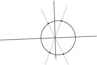
Figure 9: Principal curvature directions of a circular quadrilateral

There are deep reasons to treat circular nets as a discrete curvature line parametrization.

• The class of circular nets as well as the class of curvature line parametrized surfaces is invariant under Möbius transformations.

• Take an infinitesimal quadrilateral $(f(x,y),f(x+\epsilon),y),f(x+\epsilon),y+\epsilon),f(x,y+\epsilon))$ of a curvature line parametrized surface. A direct computation (see [11]) shows that in the limit $\epsilon\to 0$ the imaginary part of its cross-ratio is of order $\epsilon^{3}$. Note that circular quadrilaterals are characterized by having real cross-ratios.

• For any smooth curvature line parametrized surface $f:D\to{\mathbb{R}}^{3}$ there exists a family of discrete circular nets converging to $f$. Moreover the convergence is $C^{\infty}$, i.e. with all derivatives. The details can be found in [5].

One more argument in favor of Definition 3.2 is that circular nets satisfy the consistency principle, which has proven to be one of the organizing principles in discrete differential geometry [10]. The consistency principle singles out fundamental geometries by the requirement that the geometry can be consistently extended to a combinatorial grid one dimension higher. The consistency of circular nets was shown by Doliwa and Santini [16] based on the following classical theorem.

Theorem 3.3.

(Miquel) Consider a combinatorial cube in ${\mathbb{R}}^{3}$ with planar faces. Assume that three neighboring faces of the cube are circular. Then the remaining three faces are also circular.

Equivalently, provided the four-tuples of black vertices corresponding to three neighboring faces of the cube lie on circles, the three circles determined by the triples of points corresponding to three remaining faces of the cube all intersect (at the white vertex in Figure 10). It is easy to see that all vertices of Miquel’s cube lie on a sphere. Mapping the vertex shared by the three original faces to infinity by a Möbius transformation, we obtain an equivalent planar version of Miquel’s theorem. This version, also shown in Figure 10, can be proven by means of elementary geometry.

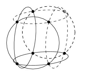
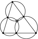
Figure 10: Miquel’s theorem: spherical and planar versions

Finally note that circular nets are also treated as a discretization of triply orthogonal coordinate systems. Triply orthogonal coordinate systems in ${\mathbb{R}}^{3}$ are maps $(x,y,z)\mapsto f(x,y,z)\in{\mathbb{R}}^{3}$ from a subset of ${\mathbb{R}}^{3}$ with mutually orthogonal $f_{x},f_{y},f_{z}$. Due to the classical Dupin theorem, the level surfaces of a triply orthogonal coordinate system intersect along their common curvature lines. Accordingly, discrete triply orthogonal systems are defined as maps from ${\mathbb{Z}}^{3}$ (or a subset thereof) to ${\mathbb{R}}^{3}$ with all elementary hexahedra lying on spheres [2]. Due to Miquel’s theorem a discrete orthogonal system is uniquely determined by the circular nets corresponding to its coordinate two-planes (see [16] and [10]).

4 Discrete Isothermic Surfaces

In this section and in the following one, we investigate discrete analogs of special classes of surfaces obtained by imposing additional conditions in terms of circles and spheres.

We start with minor combinatorial restrictions. Suppose that the vertices of $\mathcal{D}$ are colored black or white so that the two ends of each edge have different colors. Such a coloring is always possible for topological discs. To model the curvature lines, suppose also that the edges of a quad-graph $\mathcal{D}$ may consistently be labelled ‘$+$’ and ‘$-$’, as in Figure 11 (For this it is necessary that each vertex has an even number of edges).

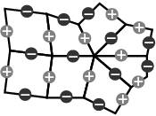
Figure 11: Labelling the edges of a discrete isothermic surface

Let $f_{0}$ be a vertex of a circular net, $f_{1},f_{3},\ldots,f_{4N-1}$ be its neighbors, and $f_{2},f_{4},\ldots,f_{4N}$ its next-neighbors (see Figure 12 (left)). We call the vertex $f_{0}$ generic if it is not co-spherical with all its neighbors and a circular net $f:{\mathcal{D}}\to{\mathbb{R}}^{3}$ generic if all its vertices are generic.

Let $f:{\mathcal{D}}\to{\mathbb{R}}^{3}$ be a generic circular net such that every its vertex is co-spherical with all its next-neighbors. We will call the corresponding sphere central. For analytical description of this geometry let us map the vertex $f_{0}$ to infinity by a Möbius transformation ${\mathcal{M}}(f_{0})=\infty$, and denote by $F_{i}={\mathcal{M}}(f_{i}),i=1,\ldots,4N$ the Möbius images of $f_{i}$. The points $F_{2},F_{4},\ldots,F_{4N}$ are obviously coplanar. The circles of the faces are mapped to straight lines. For the cross-ratios we get

$$q(f_{0},f_{2k-1},f_{2k},f_{2k+1})=\dfrac{F_{2k}-F_{2k+1}}{F_{2k}-F_{2k-1}}=\dfrac{z_{2k+1}}{z_{2k-1}},$$

where $z_{2k+1}$ is the coordinate of $F_{2k+1}$ orthogonal to the plane $\mathcal{P}$ of $F_{2},F_{4},\ldots,F_{4N}$. (Note that since $f_{0}$ is generic none of the $z_{i}$ vanishes). As a corollary we get for the product of all cross-ratios:

$$\prod_{k=1}^{n}q(f_{0},f_{2k-1},f_{2k},f_{2k+1})=1.$$ (4.1)

Figure 12: Central spheres of a discrete isothermic surface: combinatorics (left), and the Möbius normalized picture for $N=2$ (right).

Definition 4.1.

A circular net $f:{\mathcal{D}}\to{\mathbb{R}}^{3}$ satisfying condition (4.1) at each vertex is called a discrete isothermic surface.

This definition was first suggested in [6] for the case of the combinatorial square grid ${\mathcal{D}}={\mathbb{Z}}^{2}$. In this case if the vertices are labelled by $f_{m,n}$ and the corresponding cross-ratios by $q_{m,n}:=q(f_{m,n},f_{m+1,n},f_{m+1,n+1},f_{m,n+1})$, the condition (4.1) reads

$$q_{m,n}q_{m+1,n+1}=q_{m+1,n}q_{m,n+1}.$$

Proposition 4.2.

Every vertex $f_{m,n}$ of a discrete isothermic surface $f:{\mathbb{Z}}^{2}\to{\mathbb{R}}^{3}$ possesses a central sphere, i.e. the points $f_{m,n},f_{m-1,n-1},f_{m+1,n-1},f_{m+1,n+1}$ and $f_{m-1,n+1}$ are co-spherical. Moreover for generic circular maps $f:{\mathbb{Z}}^{2}\to{\mathbb{R}}^{3}$ this property characterizes discrete isothermic surfaces.

Proof.

Use the notation of Figure 12, with $f_{0}\equiv f_{m,n}$, and the same argument with the Möbius transformation $\mathcal{M}$ which maps $f_{0}$ to $\infty$. Consider the plane $\mathcal{P}$ determined by the points $F_{2},F_{4}$ and $F_{6}$. Let as above $z_{k}$ be the coordinates of $F_{k}$ orthogonal to the plane $\mathcal{P}$. Condition (4.1) yields

$$\dfrac{F_{8}-F_{1}}{F_{8}-F_{7}}=\dfrac{z_{1}}{z_{7}}.$$

This implies that the $z$-coordinate of the point $F_{8}$ vanishes, thus $F_{8}\in{\mathcal{P}}$. ∎

The property to be discrete isothermic is also 3D-consistent, i.e. can be consistently imposed on all faces of a cube. This was proven first by Hertrich-Jeromin, Hoffmann and Pinkall [23] (see also [10] for generalizations and modern treatment).

An important subclass of discrete isothermic surfaces is given by the condition that all the faces are conformal squares, i.e. their cross ratio equals $-1$. All conformal squares are Möbius equivalent, in particular equivalent to the standard square. This is a direct discretization of the definition of smooth isothermic surfaces. The latter are immersions $(x,y)\mapsto f(x,y)\in{\mathbb{R}}^{3}$ satisfying

$$\|f_{x}\|=\|f_{y}\|,f_{x}\perp f_{y},f_{xy}\in{\rm span}\{f_{x},f_{x}\},$$ (4.2)

i.e. conformal curvature line parametrizations. Geometrically this definition means that the curvature lines divide the surface into infinitesimal squares.

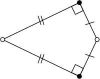
Figure 13: Right-angled kites are conformal squares

The class of discrete isothermic surfaces is too general and the surfaces are not rigid enough. In particular one can show that the surface can vary preserving all its black vertices. In this case, one white vertex can be chosen arbitrarily [7]. Thus, we introduce a more rigid subclass. To motivate its definition, let us look at the problem of discretizing the class of conformal maps $f:D\to{\mathbb{C}}$ for $D\subset{\mathbb{C}}={\mathbb{R}}^{2}$. Conformal maps are characterized by the conditions

$$|f_{x}|=|f_{y}|,\qquad f_{x}\perp f_{y}.$$ (4.3)

To define discrete conformal maps $f:\mathbb{Z}^{2}\supset D\to\mathbb{C}$, it is natural to impose these two conditions on two different sub-lattices (white and black) of $\mathbb{Z}^{2}$, i.e. to require that the edges meeting at a white vertex have equal length and the edges at a black vertex meet orthogonally. This discretization leads to the circle patterns with the combinatorics of the square grid introduced by Schramm [34]. Each circle intersects four neighboring circles orthogonally and the neighboring circles touch cyclically (Fig.14 (left)).

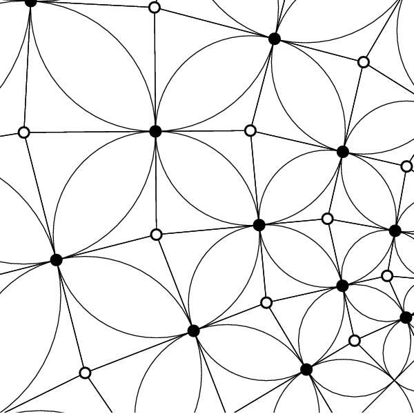
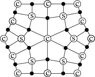
Figure 14: To the definition of discrete S-isothermic surfaces: orthogonal circle patterns as discrete conformal maps (left) and combinatorics of S-quad-graphs (right).

The same properties imposed for quadrilateral surfaces with the combinatorics of the square grid $f:\mathbb{Z}^{2}\supset{\mathcal{D}}\to{\mathbb{R}}^{3}$ lead to an important subclass of discrete isothermic surfaces. Let us require for a discrete quadrilateral surface that:

• the faces are orthogonal kites,

• the edges meet at black vertices orthogonally (black vertices are at orthogonal corners of the kites),

• the kites which do not share a common vertex are not coplanar (locality condition).

Observe that the orthogonality condition (at black vertices) implies that one pair of opposite edges meeting at a black vertex lies on a straight line. Together with the locality condition this implies that there are two kinds of white vertices, which we denote by $\bigcirc\kern-8.0ptc\$ and $\bigcirc\kern-8.0pts\$. Each kite has white vertices of both types and the kites sharing a white vertex of the first kind $\bigcirc\kern-8.0ptc\$ are coplanar.

These conditions imposed on the quad-graphs lead to S-quad-graphs and S-isothermic surfaces (the latter were introduced in [7] for the combinatorics of the square grid).

Definition 4.3.

An S-quad-graph $\mathcal{D}$ is a quad-graph with black and two kinds of white vertices such that the two ends of each edge have different colors and each quadrilateral has vertices of all kinds (see Fig. 14 (right)). Let $V_{b}({\mathcal{D}})$ be the set of black vertices. A discrete S-isothermic surface is a map

$$f_{b}:V_{b}({\mathcal{D}})\rightarrow\mathbb{R}^{3},$$

with the following properties:

1. If $v_{1},\ldots,v_{2n}\in V_{b}({\mathcal{D}})$ are the neighbors of a $\bigcirc\kern-8.0ptc\$-labeled vertex in cyclic order, then $f_{b}(v_{1}),\ldots,f_{b}(v_{2n})$ lie on a circle in $\mathbb{R}^{3}$ in the same cyclic order. This defines a map from the $\bigcirc\kern-8.0ptc\$-labeled vertices to the set of circles in $\mathbb{R}^{3}$.

2. If $v_{1},\ldots,v_{2n}\in V_{b}({\mathcal{D}})$ are the neighbors of an $\bigcirc\kern-8.0pts\$-labeled vertex, then $f_{b}(v_{1}),\ldots,$ $f_{b}(v_{2n})$ lie on a sphere in $\mathbb{R}^{3}$. This defines a map from the $\bigcirc\kern-8.0pts\$-labeled vertices to the set of spheres in $\mathbb{R}^{3}$.

3. If $v_{c}$ and $v_{s}$ are the $\bigcirc\kern-8.0ptc\$-labeled and the $\bigcirc\kern-8.0pts\$-labeled vertex of a quadrilateral of $\mathcal{D}$, then the circle corresponding to $v_{c}$ intersects the sphere corresponding to $v_{s}$ orthogonally.

Discrete S-isothermic surfaces are therefore composed of tangent spheres and tangent circles, with the spheres and circles intersecting orthogonally. The class of discrete S-isothermic surfaces is obviously invariant under Möbius transformations.

Given a discrete S-isothermic surface, one can add the centers of the spheres and circles to it giving a map $V({\mathcal{D}})\rightarrow\mathbb{R}^{3}$. The discrete isothermic surface obtained is called the central extension of the discrete S-isothermic surface. All its faces are orthogonal kites.

An important fact of the theory of isothermic surfaces (smooth and discrete) is the existence of a dual isothermic surface [6]. Let $f:{\mathbb{R}}^{2}\supset D\to{\mathbb{R}}^{3}$ be an isothermic immersion. Then the formulas

$$f^{*}_{x}=\dfrac{f_{x}}{\|f_{x}\|^{2}},\quad f^{*}_{y}=-\dfrac{f_{y}}{\|f_{y}\|^{2}}.$$

define an isothermic immersion $f^{*}:{\mathbb{R}}^{2}\supset D\to{\mathbb{R}}^{3}$ which is called the dual isothermic surface. Indeed, one can easily check that the form $df^{*}$ is closed and $f^{*}$ satisfies (4.2). Exactly the same formulas can be applied in the discrete case.

Proposition 4.4.

Suppose $f:{\mathcal{D}}\to{\mathbb{R}}^{3}$ is a discrete isothermic surface and suppose the edges have been consistently labeled ‘$+$’ and ‘$-$’, as in Fig. 11. Then the dual discrete isothermic surface $f^{*}:{\mathcal{D}}\to{\mathbb{R}}^{3}$ is defined by the formula

$$\Delta f^{*}=\pm\dfrac{\Delta f}{\|\Delta f\|^{2}},$$

where $\Delta f$ denotes the difference of values at neighboring vertices and the sign is chosen according to the edge label.

The closedness of the corresponding discrete form is elementary checked for one kite.

Proposition 4.5.

The dual of the central extension of a discrete S-isothermic surface is the central extension of another discrete S-isothermic surface.

If we disregard the centers, we obtain the definition of the dual discrete S-isothermic surface. The dual discrete S-isothermic surface can be defined also without referring to the central extension [4].

5 Discrete Minimal Surfaces and Circle Patterns: Geometry from Combinatorics

In this section (following [4]) we define discrete minimal S-isothermic surfaces (or discrete minimal surfaces for short) and present the most important facts from their theory. The main idea of the approach of [4] is the following. Minimal surfaces are characterized among (smooth) isothermic surfaces by the property that they are dual to their Gauss map. The duality transformation and this characterization of minimal surfaces carries over to the discrete domain. The role of the Gauss map is played by discrete S-isothermic surfaces whose spheres all intersect one fixed sphere orthogonally.

5.1 Koebe polyhedra

A circle packing in $S^{2}$ is a configuration of disjoint discs which may touch but not intersect. The construction of discrete S-isothermic “round spheres” is based on their relation to circle packings in $S^{2}$. The following theorem is central in this theory.

Theorem 5.1.

For every polytopal cellular decomposition of the sphere, there exists a pattern of circles in the sphere with the following properties. There is a circle corresponding to each face and to each vertex. The vertex circles form a packing with two circles touching if and only if the corresponding vertices are adjacent. Likewise, the face circles form a packing with circles touching if and only if the corresponding faces are adjacent. For each edge, there is a pair of touching vertex circles and a pair of touching face circles. These pairs touch in the same point, intersecting each other orthogonally.

This circle pattern is unique up to Möbius transformations.

The first published statement and proof of this theorem is contained in [13]. For generalizations, see [33], [31], and [9], the latter also for a variational proof.

Theorem 5.1 is a generalization of the following remarkable statement about circle packings due to Koebe [28].

Theorem 5.2.

(Koebe) For every triangulation of the sphere there is a packing of circles in the sphere such that circles correspond to vertices, and two circles touch if and only if the corresponding vertices are adjacent. This circle packing is unique up to Möbius transformations of the sphere.

Observe that, for a triangulation, one automatically obtains not one but two orthogonally intersecting circle packings, as shown in Fig. 15 (right). Indeed, the circles passing through the points of contact of three mutually touching circles intersect these orthogonally, and thus Theorem 5.2 is a special case of Theorem 5.1.

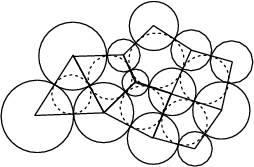
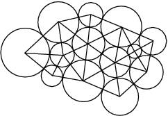
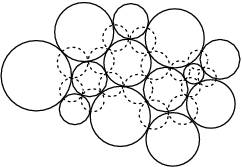
Figure 15: Left: An orthogonal circle pattern corresponding to a cellular decomposition. Middle: A circle packing corresponding to a triangulation. Right: The orthogonal circles.

Consider a circle pattern of Theorem 5.1. Associating white vertices to circles and black vertices to their intersection points, one obtains a quad-graph. Actually we have an S-quad-graph: Since the circle pattern is comprised by two circle packings intersecting orthogonally we have two kinds of white vertices, $\bigcirc\kern-8.0pts\$ and $\bigcirc\kern-8.0ptc\$, corresponding to the circles of the two packings.

Now let us construct the spheres intersecting $S^{2}$ orthogonally along the circles marked by $\bigcirc\kern-8.0pts\$. If we then connect the centers of touching spheres, we obtain a convex polyhedron, all of whose edges are tangent to the sphere $S^{2}$. Moreover, the circles marked with $\bigcirc\kern-8.0ptc\$ are inscribed in the faces of the polyhedron. Thus we have a discrete S-isothermic surface.

We arrive at the following theorem, which is equivalent to Theorem 5.1 (see also [40]).

Theorem 5.3.

Every polytopal cell decomposition of the sphere can be realized by a polyhedron with edges tangent to the sphere. This realization is unique up to projective transformations which fix the sphere.

These polyhedra are called the Koebe polyhedra. We interpret the corresponding discrete S-isothermic surfaces as conformal discretizations of the “round sphere”.

5.2 Definition of discrete minimal surfaces

Let $f:{\mathcal{D}}\to{\mathbb{R}}^{3}$ be a discrete S-isothermic surface. Suppose $x\in{\mathcal{D}}$ is a white $\bigcirc\kern-8.0pts\$ vertex of the quad-graph $\mathcal{D}$, i.e. $f(x)$ is the center of a sphere. Consider all quadrilaterals of $\mathcal{D}$ incident to $x$ and denote by $y_{1}\ldots y_{2n}$ their black vertices and by $x_{1}\ldots x_{2n}$ their white $\bigcirc\kern-8.0ptc\$ vertices. We will call the vertices $x_{1}\ldots x_{2n}$ neghboring $x$ in $\mathcal{D}$. (Generically, $n=2$.) Then $f(y_{j})$ are the points of contact with the neighboring spheres and simultaneously points of intersection with the orthogonal circles centered at $f(x_{j})$ (see Fig. 16).

Consider only the white vertices of the quad-graph. Observe that each $\bigcirc\kern-8.0ptc\$ vertex of a discrete S-isothermic surface and all its $\bigcirc\kern-8.0pts\$ neighbors are coplanar. Indeed the plane of the circle centered at $f(\mbox{$\bigcirc\kern-8.0ptc\ $})$ contains all its $f(\mbox{$\bigcirc\kern-8.0pts\ $})$ neighbors. The same condition imposed at the $\bigcirc\kern-8.0pts\$ vertices leads to a special class of surfaces.

Figure 16: To the definition of discrete minimal surfaces: the tangent plane through the center $f(x)$ of a sphere and the centers $f(x_{j})$ of the neighboring circles. The circles and the sphere intersect orthogonally at the black points $f(y_{j})$.

Definition 5.4.

A discrete S-isothermic surface $f:{\mathcal{D}}\to{\mathbb{R}}^{3}$ is called discrete minimal if for each sphere of $f({\mathcal{D}})$ there exists a plane which contains the center $f(\mbox{$\bigcirc\kern-8.0pts\ $})$ of the sphere as well as the centers $f(\mbox{$\bigcirc\kern-8.0ptc\ $})$ of all neighboring circles orthogonal to the sphere, i.e. if each white vertex of $f({\mathcal{D}})$ is coplanar to all its white neighbors. These planes should be considered as tangent planes to the discrete minimal surface.

Theorem 5.5.

An S-isothermic discrete surface $f$ is a discrete minimal surface, if and only if the dual S-isothermic surface $f^{*}$ corresponds to a Koebe polyhedron. In that case the dual surface $N:=f^{*}:V_{w}({\mathcal{D}})\to{\mathbb{R}}^{3}$ at white vertices $V_{w}({\mathcal{D}})$ can be treated as the Gauss map $N$ of the discrete minimal surface: At $\bigcirc\kern-8.0pts\$vertices $N$ is orthogonal to the tangent planes, and at $\bigcirc\kern-8.0ptc\$vertices $N$ is orthogonal to the planes of the circles centered at $f(\mbox{$\bigcirc\kern-8.0ptc\ $})$.

Proof.

That the S-isothermic dual of a Koebe polyhedron is a discrete minimal surface is fairly obvious. On the other hand, let $f:{\mathcal{D}}\rightarrow{\mathbb{R}}^{3}$ be a discrete minimal surface and let $x\in{\mathcal{D}}$ and $y_{1}\ldots y_{2n}\in{\mathcal{D}}$ be as above. Let $f^{*}:{\mathcal{D}}\rightarrow{\mathbb{R}}^{3}$ be the dual S-isothermic surface. We need to show that all circles of $f^{*}$ lie in one and the same sphere $S$ and that all the spheres of $f^{*}$ intersect $S$ orthogonally. Since the quadrilaterals of a discrete S-isothermic surface are kites the minimality condition of Definition 5.4 can be reformulated as follows: There is a plane through $f(x)$ such that the points $\{f(y_{j})\;|\;j\text{ even}\}$ and the points $\{f(y_{j})\;|\;j\text{ odd}\}$ lie in planes which are parallel to it at the same distance on opposite sides (see Fig. 16). It follows immediately that the points $f^{*}(y_{1})\ldots f^{*}(y_{2n})$ lie on a circle $c_{x}$ in a sphere $S_{x}$ around $f^{*}(x)$. The plane of $c_{x}$ is orthogonal to the normal $N$ to the tangent plane at $f(x)$. Let $S$ be the sphere which intersects $S_{x}$ orthogonally in $c_{x}$. The orthogonal circles through $f^{*}(y_{1})\ldots f^{*}(y_{2n})$ also lie in $S$. Hence, all spheres of $f^{*}$ intersect $S$ orthogonally and all circles of $f^{*}$ lie in $S$. ∎

Theorem 5.5 is a complete analogue of Christoffel’s characterization [15] of continuous minimal surfaces.

Theorem 5.6.

(Christoffel) Minimal surfaces are isothermic. An isothermic immersion is a minimal surface, if and and only if the dual immersion is contained in a sphere. In that case the dual immersion is in fact the Gauss map of the minimal surface.

Thus a discrete minimal surface is a discrete S-isothermic surface which is dual to a Koebe polyhedron; the latter is its Gauss map and is a discrete analogue of a conformal parametrization of the sphere.

The simplest infinite orthogonal circle pattern in the plane consists of circles with equal radius $r$ and centers on a square grid with spacing $\frac{1}{2}\sqrt{2}\,r$. One can project it stereographically to the sphere, construct orthogonal spheres through half of the circles and dualize to obtain a discrete version of Enneper’s surface. See Fig. 1(right). Only the circles are shown.

5.3 Construction of discrete minimal surfaces

A general method to construct discrete minimal surfaces is schematically shown in the following diagram.

continuous minimal surface

$\Downarrow$

image of curvature lines under Gauss-map

$\Downarrow$

cell decomposition of (a branched cover of) the sphere

$\Downarrow$

orthogonal circle pattern

$\Downarrow$

Koebe polyhedron

$\Downarrow$

discrete minimal surface

As usual in the theory on minimal surfaces [25], one starts constructing such a surface with a rough idea of how it should look. To use our method, one should understand its Gauss map and the combinatorics of the curvature-line pattern. The image of the curvature-line pattern under the Gauss map provides us with a cell decomposition of (a part of) $S^{2}$ or a covering. From these data, applying Theorem 5.1, we obtain a Koebe polyhedron with the prescribed combinatorics. Finally, the dualization step yields the desired discrete minimal surface. For the discrete Schwarz P-surface the construction method is demonstrated in Fig. 17 and Fig. 18.

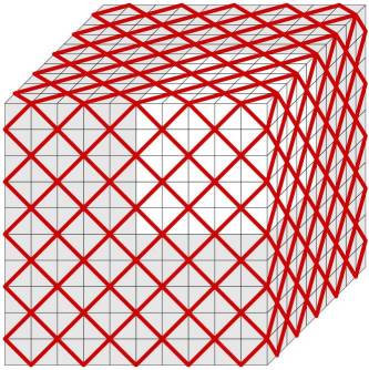
Gauss image of the curvature lines

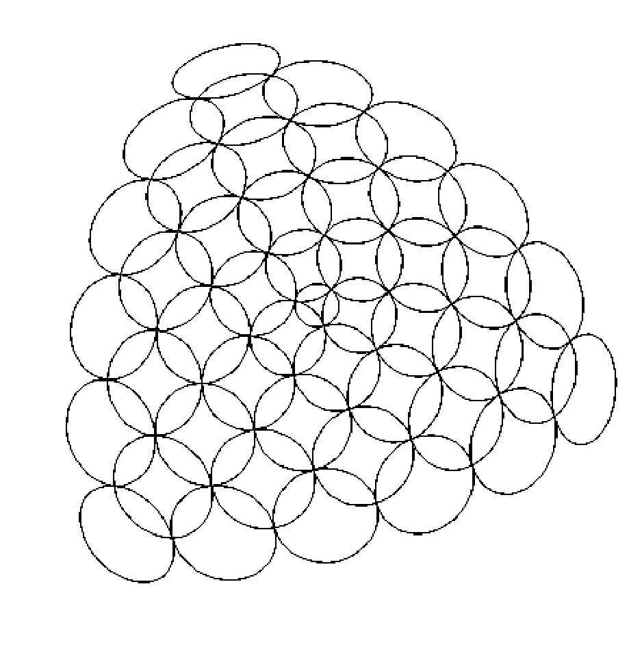
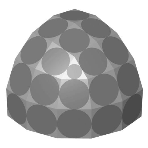
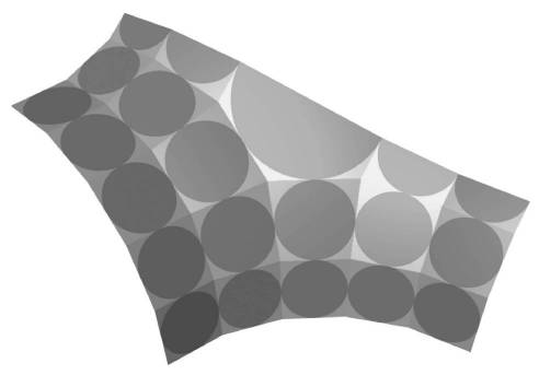
 $\rightarrow{}$ circle pattern
 $\rightarrow{}$ Koebe polyhedron  $\rightarrow{}$ discrete minimal surface

Figure 17: Construction of the discrete Schwarz P-surface.

Let us emphasize that our data, aside from possible boundary conditions, are purely combinatorial—the combinatorics of the curvature line pattern. All faces are quadrilaterals and typical vertices have four edges. There may exist distinguished vertices (corresponding to the ends or umbilic points of a minimal surface) with a different number of edges.

The most nontrivial step in the above construction is the third one listed in the diagram. It is based on the generalized Koebe Theorem 5.1. It implies the existence and uniqueness for the discrete minimal S-isothermic surface under consideration, but not only this. A constructive proof of the generalized Koebe theorem suggested in [9] is based on a variational principle and also provides a method for the numerical construction of circle patterns. An alternative algorithm by Thurston was implemented in Stephenson’s program circlepack (see [38] for an exhaustive presentation of the theory of circle packings and their numerics). The first step is to transfer the problem from the sphere to the plane by a stereographic projection. Then the radii of the circles are calculated. If the radii are known, it is easy to reconstruct the circle pattern. The above-mentioned variational method is based on the observation that the equations for the radii are the equations for a critical point of a convex function of the radii. The variational method involves minimizing this function to solve the equations.

Let us describe the variational method of [9] for construction of (orthogonal) circle patterns in the plane and demonstrate how it can be applied to construct the discrete Schwarz-P surface.

Instead of the radii $r$ of the circles, we use the logarithmic radii

$$\rho=\log r.$$

For each circle $j$, we need to find a $\rho_{j}$ such that the corresponding radii solve the circle pattern problem. This leads to the following equations, one for each circle. The equation for circle $j$ is

$$2\sum_{\makebox[0.0pt]{\scriptsize$\text{neighbors }k$}}\arctan e^{\rho_{k}-\rho_{j}}=\Phi_{j},$$ (5.1)

where the sum is taken over all neighboring circles $k$. For each circle $j$, $\Phi_{j}$ is the nominal angle covered by the neighboring circles. It is normally $2\pi$ for interior circles, but it differs for circles on the boundary or for circles where the pattern branches.

Theorem 5.7.

The critical points of the functional

$$S(\rho)=\sum_{(j,k)}\big{(}\operatorname{Im}\operatorname{Li}_{2}(ie^{\rho_{k}-\rho_{j}})+\operatorname{Im}\operatorname{Li}_{2}(ie^{\rho_{j}-\rho_{k}})-{\pi\over 2}(\rho_{j}+\rho_{k})\big{)}+\sum_{j}\Phi_{j}\rho_{j}.$$

correspond to orthogonal circle patterns in the plane with cone angles $\Phi_{j}$ at the centers of circles ($\Phi_{j}=2\pi$ for internal circles). Here, the first sum is taken over all pairs $(j,k)$ of neighboring circles, the second sum is taken over all circles $j$, and the dilogarithm function $\operatorname{Li}_{2}(z)$ is defined by $\operatorname{Li}_{2}(z)=-\int_{0}^{z}\log(1-\zeta)\,d\zeta/\zeta$. The functional is scale-invariant and restricted to the subspace $\sum_{j}\rho_{j}=0$ it is convex.

Proof.

The formula for the functional follows from (5.1) and

$$\dfrac{d}{dx}\operatorname{Im}\operatorname{Li}_{2}(ie^{x})=\dfrac{1}{2i}\log\dfrac{1+ie^{x}}{1-ie^{x}}=\arctan e^{x}.$$

The second derivative of the functional is the quadratic form

$$D^{2}S=\sum_{(j,k)}\frac{1}{\cosh(\rho_{k}-\rho_{j})}\,(d\rho_{k}-d\rho_{j})^{2},$$

where the sum is taken over pairs of neighboring circles, which implies the convexity. ∎

Now the idea is to minimize $S(\rho)$ restricted to $\sum_{j}\rho_{j}=0$. The convexity of the functional implies the existence and uniqueness of solutions of the classical boundary valued problems: Dirichlet (with prescribed $\rho_{j}$ on the boundary) and Neumann (with prescribed $\Phi_{j}$ on the boundary).

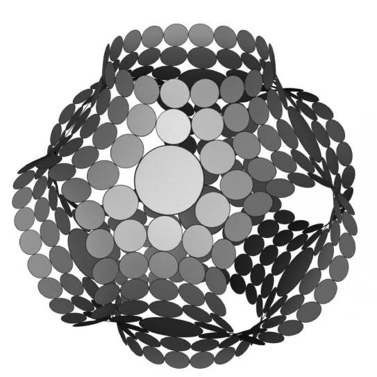
Figure 18: A discrete minimal Schwarz-P surface.

The Schwarz-P surface is a triply periodic minimal surface. It is the symmetric case in a $2$-parameter family of minimal surfaces with $3$ different hole sizes (only the ratios of the hole sizes matter), see [17]. The Gauss map is a double cover of the sphere with $8$ branch points. The image of the curvature line pattern under the Gauss map is shown schematically in Fig. 17 (top left), thin lines. It is a refined cube. More generally, one may consider three different numbers $m$, $n$, and $k$ of slices in the three directions. The $8$ corners of the cube correspond to the branch points of the Gauss map. Hence, not $3$ but $6$ edges are incident with each corner vertex. The corner vertices are assigned the label $\bigcirc\kern-8.0ptc\$. We assume that the numbers $m$, $n$, and $k$ are even, so that the vertices of the quad graph may be labelled ‘$\bigcirc\kern-8.0ptc\$’, ‘$\bigcirc\kern-8.0pts\$’, and ‘$\bullet$’ consistently (see Section 4).

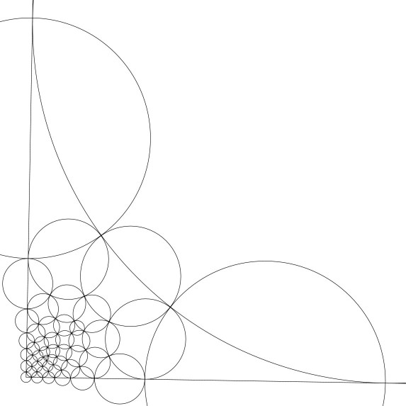
Figure 19: A piece of the circle pattern for a Schwarz-P surface after stereographic projection to the plane.

We will take advantage of the symmetry of the surface and construct only a piece of the corresponding circle pattern. Indeed the combinatorics of the quad-graph has the symmetry of a rectangular papallelepipedon. We construct an orthogonal circle pattern with the symmetry of the rectangular papallelepipedon eliminating the Möbius ambiguity of Theorem 5.1. Consider one fourth of the sphere bounded by two orthogonal great circles connecting the north and the south poles of the sphere. There are two distinguished vertices (corners of the cube) in this piece. Mapping the north pole to the origin and the south pole to infinity by stereographic projection we obtain a Neumann boundary value problem for orthogonal circle patterns in the plane. The symmetry great circles become two orthogonal straight lines. The solution of this problem is shown in Fig. 19. The Neumann boundary data are $\Phi=\pi/2$ for the lower left and upper right boundary circles and $\Phi=\pi$ for all other boundary circles (along the symmetry lines).

Now map this circle pattern to the sphere by the same stereographic projection. One half of the spherical circle pattern obtained (above the equator) is shown in Fig. 17 (top right). This is one eighth of the complete spherical pattern. Now lift the circle pattern to the branched cover, construct the Koebe polyhedron and dualize it to obtain the Schwarz-P surface; see Fig. 17 (bottom row). A translational fundamental piece of the surface is shown in Fig. 18.

We summarize these results in a theorem.

Theorem 5.8.

Given three even positive integers $m$, $n$, $k$, there exists a corresponding unique (unsymmetric) S-isothermic Schwarz-P surface.

Surfaces with the same ratios $m:n:k$ are different discretizations of the same continuous Schwarz-P surface. The cases with $m=n=k$ correspond to the symmetric Schwarz-P surface.

Further examples of discrete minimal surfaces can be found in [4] and [14].

Orthogonal circle patterns on the sphere are treated as the Gauss map of the discrete minimal surface and are central in this theory. Although circle patterns on the plane and on the sphere differ just by the stereographic projection some geometric properties of the Gauss map can get lost when represented in the plane. Moreover to produce branched circle patterns in the sphere it is important to be able to work with circle patterns directly on the sphere. A variational method which works directly on the sphere was suggested in [35, 4]. This variational principle for spherical circle patterns is analogous to the variational principles for Euclidean and hyperbolic patterns presented in [9]. Unlike the Euclidean and hyperbolic cases the spherical functional is not convex, which makes difficult to use it in the theory. However the spherical functional has proved to be amazingly powerful for practical computation of spherical circle patterns (see [4] for detail). In particular, it can be used to produce branched circle patterns in the sphere.

Numerous examples of discrete minimal surfaces are constructed with the help of the spherical functional in the contribution of Bücking [14] to this volume.

6 Discrete Conformal Surfaces and Circle Patterns

Conformal immersions

$$f:{\mathbb{R}}^{2}\supset D \to {\mathbb{R}}^{3}$$

$$(x,y) \mapsto f(x,y)$$

are characterized by the properties

$$\|f_{x}\|=\|f_{y}\|,\quad f_{x}\bot f_{y}.$$

Any surface can be conformally parametrized, and a conformal parametrization induces a complex structure on $D$ in which $z=x+iy$ is a local complex coordinate. The development of a theory of discrete conformal meshes and discrete Riemann surfaces is one of the popular topics in discrete differential geometry. Due to their almost square quadrilateral faces and general applicability, discrete conformal parametrizations are important in computer graphics, in particular for texture mapping. Recent progress in this area could be a topic of another paper; it lies beyond the scope of this survey. In this section we mention shortly only the methods based on circle patterns.

Conformal mappings can be characterized as mapping infinitesimal circles to infinitesimal circles. The idea to replace infinitesimal circles with finite circles is quite natural and leads to circle packings and circle patterns (see also Section 4). The corresponding theory for conformal mappings to the plane is well developed (see the recent book of Stephenson [38]). The discrete conformal mappings are constructed using a version of Koebe’s theorem or a variational principle which imply the corresponding existence and uniqueness statements as well as a numerical method for construction (see Section 5). It is proven that a conformal mapping can be approximated by a sequence of increasingly fine, regular circle packings or patterns [34, 22].

Several attempts have been made to generalize this theory for discrete conformal parametrizations of surfaces.

The simplest natural idea is to ignore the geometry and take only the combinatorial data of the simplicial surface [38]. Due to Koebe’s theorem there exists essentially unique circle packing representing this combinatorics. One treats it as a discrete conformal mapping of the surface. This method has been successfully applied by Hurdal et al. [26] for flat mapping of the human cerebellum. However a serious disadvantage is that the results depend only on the combinatorics and not on the geometry of the original mesh.

An extension of Stephenson’s circle packing scheme which takes the geometry into account is due to Bowers and Hurdal [12]. They treat circle patterns with non-intersecting circles corresponding to vertices of the original mesh. The geometric data in this case are the so called inversive distances of pairs of neighboring circles, which can be treated as imaginary intersection angles of circles. The idea is to get a discrete conformal mapping as a circle pattern in the plane with the inversive distances coinciding with the inversive distances of small spheres in space. The latter are centered at the vertices of the original meshes. The disadvantage of this method is that there are almost no theoretical results regarding the existence and uniqueness of inversive distance patterns.

Kharevich, Springborn and Schröder suggested another way [27] to handle the geometric data. They consider the circumcircles of the faces of a simplicial surface and take their intersection angles $\theta$. The circumcircles are taken intrinsically, i.e. they are round circles with respect to the surface metric. The latter is a flat metric with conical singularities at vertices of the mesh. The intersection angles $\theta$ are the geometric data to be respected, i.e. ideally for a discrete conformal mapping one wishes a circle pattern in the plane with the same intersection angles $\theta$. An advantage of this method is that similarly to the circle packing method it is based on a solid theoretical background — the variational principle for patterns of intersecting circles [9]. However to get a circle pattern flat one has to change the intersection angles $\theta\mapsto\tilde{\theta}$ and it seems that there is no geometric way to do this (in [27] the angles $\tilde{\theta}$ of the circle pattern in the plane are defined as minimizing the sum of differences squared $(\theta-\tilde{\theta})^{2}$). A solution to this problem could possibly be achieved by a method based on Delaunay triangulations of circle patterns with disjoint circles. The corresponding variational principle has been found recently in [36].

It seems that discrete conformal surface parametrizations are at the beginning of a promising development. Although now only some basic ideas about discrete conformal surface parametrizations have been clarified and no approximation results are known, there is good chance for a fundamental theory with practical applications in this field.

References

- [1] W. Blaschke, Vorlesungen über Differentialgeometrie III, Die Grundlehren der mathematischen Wissentschaften, Berlin: Springer-Verlag, 1929.
- [2] A.I. Bobenko, Discrete conformal maps and surfaces, Symmetries and Integrability of Difference Equations (P.A. Clarkson and F.W. Nijhoff, eds.), London Mathematical Society Lecture Notes Series, vol. 255, Cambridge University Press, 1999, pp. 97–108.
- [3] , A conformal functional for simplicial surfaces, Combinatorial and Computational Geometry (J.E. Goodman, J. Pach, and E. Welzl, eds.), MSRI Publications, vol. 52, Cambridge University Press, 2005, pp. 133–143.
- [4] A.I. Bobenko, T. Hoffmann, and B.A. Springborn, Minimal surfaces from circle patterns: Geometry from combinatorics, Annals of Math. 164(1) (2006), 1–34.
- [5] A.I. Bobenko, D. Matthes, and Y.B. Suris, Discrete and smooth orthogonal systems: -approximation, Internat. Math. Research Notices 45 (2003), 2415–2459.
- [6] A.I. Bobenko and U. Pinkall, Discrete isothermic surfaces, J. reine angew. Math. 475 (1996), 187–208.
- [7] , Discretization of surfaces and integrable systems, Discrete integrable geometry and physics (A.I. Bobenko and R. Seiler, eds.), Oxford Lecture Series in Mathematics and its Applications, vol. 16, Clarendon Press, Oxford, 1999, pp. 3–58.
- [8] A.I. Bobenko and P. Schröder, Discrete Willmore flow, Eurographics Symposium on Geometry Processing (2005) (M. Desbrun and H. Pottmann, eds.), The Eurographics Association, 2005, pp. 101–110.
- [9] A.I. Bobenko and B.A. Springborn, Variational principles for circle patterns and Koebe’s theorem, Transactions Amer. Math. Soc. 356 (2004), 659–689.
- [10] A.I. Bobenko and Yu.B. Suris, Discrete Differential Geometry. Consistency as Integrability, 2005, arxiv:math.DG/0504358, preliminary version of a book.
- [11] A.I. Bobenko and S.P. Tsarev, Curvature line parametrization from circle patterns, 2007, arXiv:0706.3221.
- [12] P.L. Bowers and M.K. Hurdal, Planar conformal mappings of piecewise flat surfaces, Visualization and Mathematics III. (H.-C. Hege and K. Polthier, eds.), Springer-Verlag, 2003, pp. 3–34.
- [13] G.R. Brightwell and E.R. Scheinerman, Representations of planar graphs, SIAM J. Disc. Math. 6(2) (1993), 214–229.
- [14] U. Bücking, Minimal surfaces from circle patterns: Boundary value problems, examples, this volume.
- [15] E. Christoffel, Über einige allgemeine Eigenschaften der Minimumsflächen, J. reine angew. Math. 67 (1867), 218–228.
- [16] J. Cieslinski, A. Doliwa, and P.M. Santini, The integrable discrete analogues of orthogonal coordinate systems are multi-dimensional circular lattices, Phys. Lett. A 235(5) (1997), 480–488.
- [17] U. Dierkes, S. Hildebrandt, A. Küster, and O. Wohlrab, Minimal surfaces I., Grundlehren der mathematischen Wissenschaften, vol. 295, Berlin: Springer-Verlag, 1992.
- [18] W. Fenchel, Über Krümmung und Windung geschlossener Raumkurven, Math. Ann. 101 (1929), 238–252.
- [19] E. Grinspun, A discrete model of thin shells, this volume.
- [20] E. Grinspun, A.N. Hirani, M. Desbrun, and P. Schröder, Discrete shells, Eurographics/SIGGRAPH Symposium on Computer Animation (D. Breen and M. Lin, eds.), The Eurographics Association, 2003, pp. 62–67.
- [21] B. Grünbaum, Convex Polytopes, Graduate Texts in Math., vol. 221, Springer-Verlag, New York, 2003, Second edition prepared by V. Kaibel, V. Klee and G. M. Ziegler (original edition: Interscience, London 1967).
- [22] Z.-X. He and O. Schramm, The -convergence of hexagonal disc packings to the Riemann map, Acta Math. 180 (1998), 219–245.
- [23] U. Hertrich-Jeromin, T. Hoffmann, and U. Pinkall, A discrete version of the Darboux transform for isothermic surfaces, Discrete integrable geometry and physics (A.I. Bobenko and R. Seiler, eds.), Oxford Lecture Series in Mathematics and its Applications, vol. 16, Clarendon Press, Oxford, 1999, pp. 59–81.
- [24] C.D. Hodgson, I. Rivin, and W.D. Smith, A characterization of convex hyperbolic polyhedra and of convex polyhedra inscribed in a sphere, Bull. Am. Math. Soc., New Ser. 27 (1992), 246–251.
- [25] D. Hoffman and H. Karcher, Complete embedded minimal surfaces of finite total curvature, Geometry V: Minimal surfaces (R. Osserman, ed.), Encyclopaedia of Mathematical Sciences, vol. 90, Springer-Verlag, Berlin, 1997, pp. 5–93.
- [26] M. Hurdal, P.L. Bowers, K. Stephenson, D.W.L. Sumners, K. Rehm, K. Schaper, and D.A. Rottenberg, Quasi-conformality flat mapping the human cerebellum, Medical Image Computing and Computer-Assisted Intervention, Springer-Verlag, 1999, pp. 279–286.
- [27] L. Kharevich, B. Springborn, and P. Schröder, Discrete conformal mappings via circle patterns, ACM Transactions on Graphics 25:2 (2006), 1–27.
- [28] P. Koebe, Kontaktprobleme der konformen Abbildung, Abh. Sächs. Akad. Wiss. Leipzig Math.-Natur. Kl. 88 (1936), 141–164.
- [29] R.R. Martin, J. de Pont, and T.J. Sharrock, Cyclide surfaces in computer aided design, The Mathematics of Surfaces (J. Gregory, ed.), The Institute of Mathematics and its Applications Conference Series. New Series, vol. 6, Clarendon Press, Oxford, 1986, pp. 253–268.
- [30] A.W. Nutbourne, The solution of a frame matching equation, The Mathematics of Surfaces (J. Gregory, ed.), The Institute of Mathematics and its Applications Conference Series. New Series, vol. 6, Clarendon Press, Oxford, 1986, pp. 233–252.
- [31] I. Rivin, A characterization of ideal polyhedra in hyperbolic 3-space, Ann. of Math. 143 (1996), 51–70.
- [32] R. Sauer, Differenzengeometrie, Berlin: Springer-Verlag, 1970.
- [33] O. Schramm, How to cage an egg, Invent. Math. 107(3) (1992), 543–560.
- [34] , Circle patterns with the combinatorics of the square grid, Duke Math. J. 86 (1997), 347–389.
- [35] B.A. Springborn, Variational principles for circle patterns, Ph.D. thesis, TU Berlin, 2003, arXiv:math.GT/0312363.
- [36] , A variational principle for weighted Delaunay triangulations and hyperideal polyhedra, 2006, arXiv:math.GT/0603097.
- [37] E. Steinitz, Über isoperimetrische Probleme bei konvexen Polyedern, J. reine angew. Math. 159 (1928), 133–143.
- [38] K. Stephenson, Introduction to circle packing: The theory of discrete analytic functions, Cambridge University Press, 2005.
- [39] T.J. Willmore, Riemannian geometry, Oxford Science Publications, 1993.
- [40] Günter M. Ziegler, Lectures on Polytopes, Graduate Texts in Mathematics, vol. 152, Springer-Verlag, New York, 1995, Revised edition, 1998.