Hubble diagram of gamma-ray bursts calibrated with Gurzadyan-Xue cosmology

Abstract

Aims.

Methods.

Results.

Abstract

Context. Gamma-ray bursts (GRBs) being the most luminous among known cosmic objects carry an essential potential for cosmological studies if properly used as standard candles.

Aims. In this paper we test with GRBs the cosmological predictions of the Gurzadyan-Xue (GX) model of dark energy, a novel theory that predicts, without any free parameters, the current vacuum fluctuation energy density close to the value inferred from the SNIa observations. We also compare the GX results with those predicted by the concordance scenario $\Lambda$-CDM.

Methods. According to the statistical approach by Schaefer (2007), the use of several empirical relations obtained from GRBs observables, after a consistent calibration for a specific model, enables one to probe current cosmological models. Based on this recently introduced method, we use the 69 GRBs sample collected by Schaefer (2007); and the most recently released SWIFT satellite data (Sakamoto et al. 2007) together with the 41 GRBs sample collected by Rizzuto et al. (2007), which has the more firmly determined redshifts. Both data samples span a distance scale up to redshift about 7.

Results. We show that the GX models are compatible with the Hubble diagram of the Schaefer (2007) 69 GRBs sample. Such adjustment is almost identical to the one for the concordance $\Lambda$-CDM. ¿From this particular analysis we can obtain the corresponding values of the matter density parameter $\Omega_{m}$ describing GX models. When the similar procedure is applied to the Rizzuto et al. (2007) and Sakamoto et al. (2007) SWIFT satellite data, we verify that the SWIFT sample does not delineate a Hubble diagram as clearly as featured by the 69 GRBs sample.

Conclusions. The analysis of the samples of Schaefer (2007) and those by Rizzuto et al. (2007) and of SWIFT (Sakamoto et al. 2007) shows that more data and efforts are needed to elucidate both issues: the gamma-ray bursts/standard-candle and lack of a theoretical understanding of the physics subjacent to the empirical relations.

1 Introduction

Recently Gamma-Ray Bursts (GRBs) were used for cosmography aims, for the analyses of the high-redshift behavior of the $\Lambda$-CDM cosmological scenario, as well as for several alternative cosmologies (see Schaefer (2003, 2007); Bloom, et al. (2003); Dai, et al. (2004); Ghirlanda, et al. (2004); Friedman & Bloom (2005); Liang & Zhang (2005, 2006); Xu et al (2005); Wang & Dai (2006); Firmani, et al. (2006); and other papers). The potential power of GRBs for cosmological studies, obviously, resides both in their very high luminosity, which the highest among known astrophysical objects, and the fact that they undergo practically no extinction over cosmological distances. Hence, one can get the possibility to trace significantly higher distance scales than it is possible via supernovae, that is, to trace very deep in the expansion history of the universe. The situation however, not as simple.

Schaefer (2007) has developed a statistical approach based on the empirical correlations obtained from several observed GRBs characteristics and obtained the Hubble diagram for the GRBs after calibrated them for the concordance and other cosmological models. This approach has been used also in (Cuesta, et al. (2007)). The key issue is the use of the empirical relations, e.g. of Ghirlanda, Liang-Zhang and others, in the absence of understanding of their underlying nature, i. e., the genuine character of the scatter in the GRBs luminosity vs. luminosity indicators relations and of their mutual links. To this difficulty Schaefer (2007) has shown that, although the scatter of each of empirical relations can be not as small, their joint action can lead to a smaller scatter, useful for probing certain cosmological models. Increase of the statistics and deeper studies of the systematics and selection effects will certainly increase the informativity of Schaefer’s approach.

In the present paper we use the same approach as Schaefer (2007), to obtain the gamma-ray burst Hubble diagram for the cosmological models proposed by Gurzadyan and Xue (2003). The original motivation for GX cosmological models is the fact that, they predict the current vacuum fluctuation energy density close to the value inferred from the SNIa observations (Perlmutter (1998); Riess, et al. (1998); Perlmutter (1999); Riess, et al. (2004, 2006)) without any free parameter.

2 The Cosmological Models

Gurzadyan and Xue (2002, 2003) have derived a formula for the dark energy, which fits the observed value without free parameters

$$\rho_{GX}=\frac{\pi}{8}\frac{\hbar c}{L_{p}^{2}}\frac{1}{a^{2}}=\frac{\pi}{8}\frac{c^{4}}{G}\frac{1}{a^{2}},$$ (1)

where $\hbar$ is the Planck constant, the Planck length is $L_{p}=\left(\hbar G\right)^{\frac{1}{2}}c^{-3/2}$, $c$ is the speed of light, and $G$ is the gravitational constant. Here $a$ is the upper cutoff scale in computation of vacuum fluctuations and has to be close to the event horizon (Djorgovski & Gurzadyan (2006)). According to (Zeldovich (1968)), the vacuum energy (1) corresponds to the cosmological term.GX formula (1) defines a broad set of cosmological models (Vereshchagin (2006)). For the latter the existence of a separatrix was shown (Vereshchagin & Yegorian (2006a)), which divides the space of cosmological solutions into two classes: Friedmannian-like with initial singularity and non-Friedmannian solutions which begin with nonzero scale factor and vanishing matter density. Each solution is characterized by the single quantity, a density parameter which is defined in the same way as in the standard cosmological model $\Omega_{m}=\frac{8\pi G_{0}\mu_{0}}{3H_{0}^{2}},$ where $\mu$ is the matter density, $H$ is the Hubble parameter, and index ”$0$” refers to their values today. The separatrix is given by

$$\Omega_{sep}=\frac{2}{3}\frac{1}{1-\frac{K}{\pi^{2}}}\approx\frac{2}{3},$$ (2)

where $K=\pm 1,0$ parametrize the spatial curvature. The origin of the separatrix was revealed in (Khachatryan (2007)), and attributed to existence of invariants in GX models.

Analytical solutions for the GX models both for matter density and the scale factor are obtained (Vereshchagin & Yegorian (2006b)). It turns out that the most simple solutions for the scale factor are again those of the separatrix. In one model it is exponential, in the others they are polynomials. Vereshchagin and Yegorian (2006b, 2008) generalized GX models to include radiation and looked for other consequences of the models.

The predictions of the GX models were shown to be compatible to supernovae and Cosmic Microwave Background data in (Djorgovski & Gurzadyan (2006)). A likelihood analysis of supernovae and radio galaxies data was performed in (Vereshchagin & Yegorian (2006c), Khachatryan, et al. (2007)).

3 Luminosity Distance Formula for GX-models

The models are described by the two equations for the mass density and scale factor (Vereshchagin & Yegorian (2006b))

$$\dot{\mu}+3H\left(\mu+\frac{p}{c^{2}}\right)=-\dot{\mu}_{\Lambda}+\left(\mu+\mu_{\Lambda}\right)\left(\frac{2\dot{c}}{c}-\frac{\dot{G}}{G}\right),$$

$$H^{2}+\frac{kc^{2}}{a^{2}}-\frac{\Lambda}{3}=\frac{8\pi G}{3}\mu,$$ (3)

where a dot denotes time derivative. For matter (pressure $p=0$) we have solution for matter mass density with GX-dark energy (Khachatryan (2007))

$$\mu_{m}(t)=\left(b_{m}^{GX}+\frac{\pi a(t)}{4}\right)\frac{c^{2}(t)}{G(t)a^{3}(t)},$$ (4)

where $b_{m}$ is a GX-invariant for matter. For the scale factor

$$\dot{a}(t)=c(t)\sqrt{\frac{8\pi b_{m}^{GX}}{3a(t)}+\pi^{2}-k}.$$ (5)

The luminosity distance $d_{L}$ is (Peebles (1993); Daly & Djorgovski (2005))

$$d_{L}(z)=a_{0}f_{k}(\kappa_{s})(1+z),$$

$$\kappa_{s}=\frac{1}{a_{0}H_{0}}\int_{0}^{z}\frac{c(\acute{z})}{h(\acute{z})}d\acute{z},$$

$$h(z)=\frac{H(z)}{H_{0}},1+z=\frac{a_{0}}{a}$$

where $\kappa_{s},z$ are normalized distance and redshift, respectively. The function $f_{k}(\kappa_{s})$ is defined as

$$f_{k}(x)=\left\{\begin{array}[c]{c}\sin(x),k=1,\\ x,k=0,\\ \sinh(x),k=-1,\end{array}\right.$$ (6)

here $k$ is the effective curvature $K-\pi^{2}/3$ as in (2). The luminosity distance $d_{L}(z)$ for GX models

$$d_{L}(z)=a_{0}(1+z)f_{k}\left(\frac{1}{\sqrt{\beta}}\ln\left|\frac{g(z)-1}{g(0)-1}\,\,\frac{g(0)+1}{g(z)+1}\right|\right),$$ (7)

where

$$g(z)=\sqrt{\frac{\alpha}{\beta}(z+1)+1},\hskip 8.5359pt\alpha=\frac{8\pi b_{m}^{GX}}{3a_{0}}\;,\hskip 8.5359pt\beta=\pi^{2}-k\;.$$ (8)

For the separatrix $\alpha=b_{m}^{GX}=0$ we have a simple equation for the luminosity distance

$$d_{L}(z)=a_{0}(1+z)f_{k}\left(\frac{\ln|z+1|}{\sqrt{\pi^{2}-k}}\right).$$ (9)

4 Gamma Ray Bursts calibrated with GX models

For the present analysis we benefit of the largest GRBs sample having properly determined redshifts and luminosities currently available. The first was constructed by Schaefer (2007) and includes 69 GRBs whose main observables: time lag, variability, peak energy, maximum energy in $\gamma$-rays and rise time, which were obtained from the GRBs data provided by many $\gamma$-ray and X-ray satellites, and ground-based observatories, as collected in Greiner’s homepage: http://www.mpe.mpg.de/ jcg/grbgen.html The second one is the 41 GRBs sample with firmly determined redshift as collected by Rizzuto et al. (2007) from the SWIFT satellite.

We performed the calibration procedure (linear regression analysis) of five luminosity relations: time lag vs. luminosity ($\tau_{\text{\tiny lag}}-L$), variability vs. luminosity ($V-L$), peak energy vs. luminosity ($E_{\textrm{peak}}-L$), peak energy vs. geometrically corrected gamma-ray energy ($E_{\textrm{peak}}-E_{\gamma}$), and risetime vs. luminosity ($\tau_{\text{\tiny RT}}-L$) (Schaefer (2007); Cuesta, et al. (2007)). We use the OLS Bisector method (Isobe et al. (1999)) to find a relation between each pair of these GRBs observational properties. The best-fit line for all luminosity relations is given by the general expression $\log{\cal L}=a+b\log{{\cal I}},$ where $\cal L$ is the luminosity and $\cal I$ is the luminosity indicator, and $a$ is the intercept and $b$ is the slope in each of the calibration plots here presented. Their uncertainties are:

$$\sigma^{2}_{{\log(L_{i})}}=\sigma^{2}_{a}+(\sigma_{b}\,x_{i})^{2}+(b\,\sigma_{x_{i}})^{2}+\sigma^{2}_{\text{\tiny sys}}\;,$$ (10)

where $\sigma_{\log{L_{i}}}$ defines the standard deviation in the luminosity ${L_{i}}$, $\sigma_{a}$ is the standard deviation in the intercept $a$, $\sigma_{b}$ is the standard deviation in the intercept $b$, $\sigma_{x_{i}}$ is the standard deviation in each $x_{i}$ variable representing $\log{I}$, and $\sigma_{\text{\tiny sys}}$ is the systematic error associated to each luminosity ${L_{i}}$ estimate. The results of the calibration procedure are given in the Table 1, and the plot for all luminosity relations is given in the Fig. (1).

Table 1: Calibration Results

Luminosity Relation	$a$	$\sigma_{a}$	$b$	$\sigma_{b}$	$\sigma_{\text{\tiny sys}}$
$\tau_{\text{lag}}-L$	52.20	0.07	-1.01	0.09	0.36
$V-L$	52.41	0.08	1.78	0.19	0.47
$E_{\textrm{peak}}$-$L$	52.15	0.05	1.69	0.10	0.41
$E_{\textrm{peak}}$-Eγ	50.49	0.05	1.62	0.11	0.21
$\tau_{\text{\tiny RT}}-L$	52.45	0.07	-1.22	0.11	0.47

(a) Time lag vs. $L$

(b) Variability vs. $L$

(c) $E_{\textrm{peak}}$  vs. $L$

(d) $E_{\textrm{peak}}$  vs. E_γ  (Ghirlanda Relation)

(e) Rise time vs. $L$

Figure 1: COLOR-ONLINE Results of the calibration procedure. Notice that all relations were corrected to the rest frame of the GRB and also by using the luminosity best-fit line obtained from the nonlinear regression method. (a) Time lags for 39 GRBs. (b) Variability for 51 GRBs vs. isotropic luminosity. (c) $E_{\textrm{peak}}$  values for 64 GRBs vs. isotropic luminosity. (d) $E_{\textrm{peak}}$ values for 27 GRBs vs. total burst energy in the gamma rays. (e) Rise time for 62 GRBs vs. isotropic luminosity.

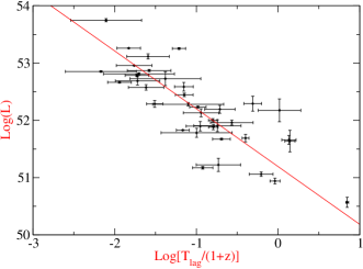
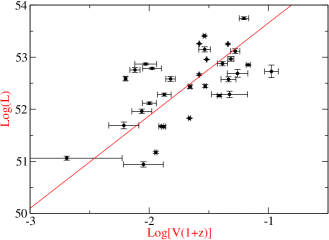
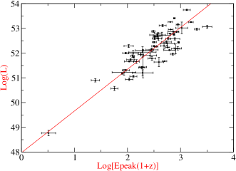
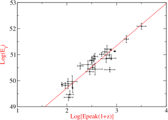
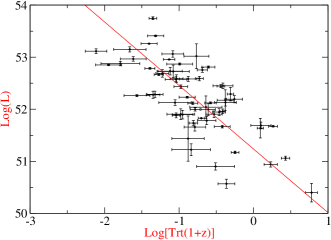
Using the same method as Schaefer (2007), we obtained the best estimated distance moduli $\mathrm{bar}{\mu}_{i}$

$$\mathrm{bar}{\mu}=\frac{1}{w}\sum_{i=1}^{5}w_{i}\mathrm{bar}{\mu}_{i},\quad w_{i}=1/\sigma^{2}_{i}\quad\textrm{and}\quad\left[w=\sum_{i=1}^{5}w_{i}\right]\;,$$ (13)

where the summation is over the relations with available data, $\mathrm{bar}{\mu}_{i}$ is the best estimated distance modulus from the $i$-th relation, and $\sigma_{i}$ is the corresponding uncertainty. Then applying the error propagation law to the equation (13) we obtained the standard deviation associated to this best estimated as $\sigma_{\mathrm{bar}{\mu}}=1/\sqrt{w}$.

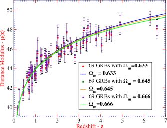
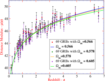
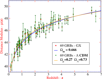
The Fig.(3) presents the Hubble Diagram for the 69 GRBs calibrated with the GX models and its comparison with the $\Lambda$-CDM model, for the parameters given in the inset. Fig.(2) shows the Hubble Diagram for the 69 GRBs calibrated with the GX models obtained after a slight variation of the separatrix solution for each cosmological model, i.e., depending on the curvature $k=0,-1$.

(a) k = 0

(b) k = -1

Figure 2: COLOR-ONLINE Hubble Diagram of 69 GRBs calibrated with GX models. (a) Case $k=0$ and different values of $\Omega_{\textrm{m}}$. (b) Case $k=-1$ and different values of $\Omega_{\textrm{m}}$. The corresponding parameters are indicated in the insets.

Figure 3: COLOR-ONLINE Hubble diagram of 69 GRBs calibrated with GX models as obtained from the empirical relations provided by Fig.-1. The blue line represents GX models calibrated with $\Omega_{\textrm{m}}=0.66$,  $k=0$ and $H_{0}=70$  k m   s M . Orange line is for the concordance cosmology $\Omega_{\textrm{m}}=0.27$, $\Omega_{\Lambda}=0.73$.

5 Results

5.1 GX compatibility with the 69 GRBs sample

We now compare GX models with the data set of 69 GRBs of Schaefer (2007). We use general least square technique for all models with different density and curvature parameters. We find the best fit as $\Omega_{m}=2/3,\,\,k=0$. The $\chi^{2}$ value for that parameters is $1.037$ with 68 DoF. The best fit curve is shown in Fig.(4(a)) for the value of the curvature parameter $k=0$, while in Fig.(4(b)) the best fit curve is shown for $k=-1$. In both figures, which combine gamma-ray bursts, supernova type Ia and radio-galaxies, several other HD from the GX model are plotted for different parameter $\Omega_{m}$, as indicated. Notice that the discrete set of data in the curves of Fig.(5) are due to the lack of an extensive study in the parameter space of $\Omega_{m}$. We plan to address this point in a forthcoming communication.

(a) k = 0

(b) k = -1

Figure 4: COLOR-ONLINE a) The Hubble diagram for SNIa, radio-galaxies (RG), and GRBs calibrated both with GX model with $k=0$, $H_{0}=70$  k m   s M , and $\Lambda$-CDM with $H_{0}=73$  k m   s M . SNIa: green points. RG: magenta points. GRBS: red points and black error bars. b) Hubble diagram for GX with $k=-1$ and $H_{0}=70$  k m   s M

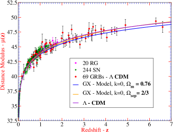
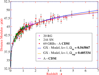
For the same parameters we have $\chi^{2}\approx 2$ with 264 DoF for SN (Khachatryan, et al. (2007)). The pair best fit values of the matter density parameter are close to the separatrix value for $k=0,-1,1$, which once again shows the important role of the separatrix in GX models. Indeed, we see that the separatrix fits the best the observational data, with the shown values of the matter density parameter $\Omega_{m}$ and the curvature $k$.

Figure 5: COLOR-ONLINE $\chi^{2}$ for the Hubble diagrams vs the $\Omega_{m}$ for $k=0,-1,1$ GX-models. The fit points (circles) correspond to the separatrix.

Concerning the $k=-1$ models, let us note that the ellipticity detected in the Cosmic Microwave Background radiation temperature maps is characteristic of photon beam motion in hyperbolic spaces (Gurzadyan et al 2005, 2007). Thus, it can act as a model-independent indication of the non precisely zero curvature of the Universe (Penrose 2005, Wiltshire 2007).

5.2 GX compatibility with the 41 SWIFT Satellite GRBs sample

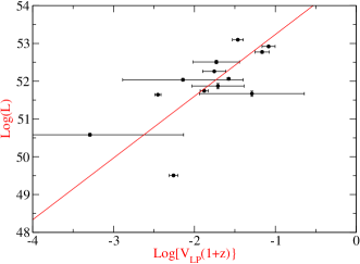
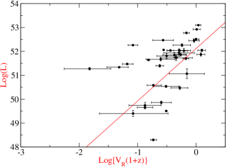
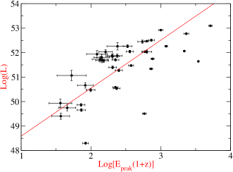
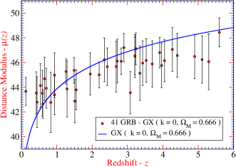
In this section we use the recently released SWIFT satellite, BAT instrument GRBs data (Sakamoto et al. 2007), namely, a sample of 41 GRBs known to have firmly determined redshifts (Rizzuto et al. 2007). We performed a similar procedure as Schaefer (2007), by constructing only three (3) luminosity indicator empirical relations from the SWIFT data. In particular by using the two variabilities defined by Rizzuto et al. (2007), which were constructed taking into account the specific operational characteristics of the BAT instrument when analyzing the GRBs mask-tagged light curves. Those luminosity vs. luminosity indicator empirical relations are as follows [see a more detailed discussion, definitions and references in Rizzuto et al. (2007)]:

• Luminosity vs. Indicator: $V_{\rm R}$ Variability.— We built this relation based on data of $V_{\rm R}$ variability provided by Rizzuto et al. (2007) and SWIFT Flux data from Sakamoto et al. (2007). Rizzuto et al. (2007) proved that a Poissonian variance describes the statistical fluctuations of the GRBs light curves (see Apendix A in Rizzuto et al. 2007). The main reason is that the count rates that were used in the analysis already had their background substracted

• Luminosity vs. Indicator: Peak Luminosity.— This relation was constructed for each GRBs as given in Table 1. of Rizzuto et al. (2007), which was obtained after extracting the mask-tagged light curve by using a binning time of 50 ms in the energy band [15-350] KeV (redshift corrected). The 1 s time interval with the highest total counts was found, and assumed as the time interval corresponding to 1 s peak count rate in the subsequent analysis

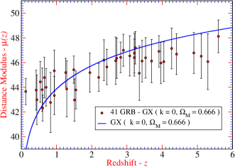
• Luminosity vs. Indicator: $V_{\rm LP}$ Variability.— The same procedure as above, but notice that it was supposed that no extra-Poissonian variance had to be substracted from the already mask-tagged light curves

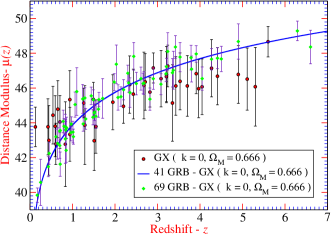
Our results for the SWIFT GRBs data analysis are presented in the Figure-6, where the three empirical relations (6(a) $V_{\rm LP}$ vs. $L$, 6(b) $V_{\rm R}$ vs. $L$, 6(c) $E_{\textrm{peak}}$  vs. $L$) described above are plotted. Besides, Fig.(6d-6f) present three Hubble diagrams obtained by varying the normalization constant in the variability relations. Notice that Fig.(6e) combines the SWIFT and Schaefer 69 GRBs data. These figures summarize the whole process of testing the consistency of the GX model (for several values of the parameters $k$ and $\Omega_{m}$) with SWIFT GRBs data, as shown in Tables 3-11. The attentive reader should bear in mind that only three of those calibration processes are illustrated in Figure-6. Fig.(6d-6f) reveal also the sensitivity of the calibration procedure for these definitions of the GRBs variability on the normalization constant. The combined HD in Fig(6e) appears to be still consistent with the GX cosmological model, but it is also clear that the SWIFT GRBs data distort the better delineate HD of the Schaefer’s 69 GRBs sample. This suggests that more data of high redshift GRBs detected by SWIFT would be needed to clarify the viability of using them as insight into GRBs precision cosmology. In this respect, perhaps the use of the SWIFT 77 GRBs sample with measured redshifts collected by Butler et al. (2007) may be of some help. That sample upon arrival of other new datasets will be used in future studies.

(a) Variability $V_{\rm LP}$ vs. $L$

(b) Variability $V_{\rm R}$ vs. $L$

(c) $E_{\textrm{peak}}$  vs. $L$

(d) Hubble diagram

(e) HD for $V_{\rm R}$, $V_{\rm LP}$ with equal normalization constant 0.05

(f) HD for $V_{\rm R}$, $V_{\rm LP}$ with different normalization constant

Figure 6: COLOR-ONLINE Results of the calibration procedure for the SWIFT satellite 41 GRBs with redshift firmly determined (Rizzuto et al. 2007). Notice that all relations were corrected to the rest frame of the GRB and also by using the luminosity best-fit line obtained from the nonlinear regression method. (a) Variability $V_{\rm LP}$ for 13 GRBs vs. isotropic luminosity. (b) Variability $V_{\rm R}$ for 37 GRBs vs. isotropic luminosity. (c) $E_{\textrm{peak}}$  values for 41 GRBs vs. peak isotropic luminosity. (d) Hubble diagram (HD) from above relations with $V_{\rm R}=V_{\rm LP}$ normalization constant 0.02. (e) HD combining 41 SWIFT and 69 Schaefer’s GRBs samples, using $V_{\rm R}$, $V_{\rm LP}$ variabilities with equal normalization constant 0.05. (f) $V_{\rm R}$, $V_{\rm LP}$ variabilities with different normalization constant

6 Conclusion

We have used the approach by Schaefer (2007) to obtain the gamma-ray bursts Hubble diagram for the cosmological GX models with dark energy. We have shown their fit to the observational data of GRBs with redshift up to $z\sim 6$, and have obtained the best fit values for the parameter $\Omega_{m}$ defining the models, see Table 2; e.g. the best fits for GRB69 correspond to $\Omega_{m}=0.64\pm 0.005$, for SN+RG $\Omega_{m}=0.508\pm 0.004$.

Since GX-models predict the current value of dark energy defining from SN1a data, this fact is remarkable in the context of degeneracy between the cosmological parameters.

Table 2: The confidence levels for the used datasets separately and together, with corresponding values of $\Omega_{m}$; all cases are for $k=0$.

Sample	$\chi^{2}$	$\Omega_{m}$
SN244+RG20	1.23	0.508
GRB69	1.04	0.64
GRB41	1.41	0.66
SN244+RG20+GRB69	1.58	0.66
GRB69+GRB41	1.16	0.66
GRBAll+SN244+RG20	1.56	0.66

The key issue in such an analysis is up to which extent the gamma-ray bursts can be used as standard candles, i. e. in revealing of the genuine scatter in the empirical relations used for obtaining the Hubble diagram. Given the lack in the understanding of the physics of those relations, handling the new data (Sato et al 2007; Sakamoto et al 2007; Rizzuto et al 2007) must need a particular care. For example, recently Campana et al (2007) claimed weakening of the Ghirlanda relation ($\chi^{2}$ up to 2 or 3) using a sample of 5 bursts observed by SWIFT. Even assuming that this result is correct, it will influence our evaluations negligibly ($\chi^{2}=1.040$ instead of 1.037). However, Ghirlanda et al (2007) reconsidered the same SWIFT sample and showed that, that relation survives practically unmodified. Recently also Cabrera et al (2007) have reported the correspondence of a sample of SWIFT data with those of other satellites and, hence, absence of outliers.

In sum, the preliminary character of testing of cosmological models via the gamma-ray burst Hubble diagram indeed remains until the understanding of the nature of the used empirical relations and availability of more observational data.

We thank the referee for many helpful comments. The last three authors are partially supported by INTAS.

Table 3: Calibration relations for the GX cosmological model with parameters $k$ and $\Omega_{m}$ as indicated. $A$ and $B$ represent the linear regression intersept and slope as defined in the text, while $\sigma_{A}$ and $\sigma_{B}$ represent their respective errors, obtained through the linear regression after using the SLOPES method. Here $L$ is the luminosity, $\tau_{\text{\tiny lag}}$ is the time lag, $V$ is the variability, $E_{peak}$ is the peak (or maximum) energy, $E_{\gamma}$ is the corresponding energy in gamma-rays, and $\tau_{RT}$ is the rise-time.

Luminosity Relation	A	B	$\sigma_{A}$	$\sigma_{B}$
$k=0,\,\,\Omega_{m}=0.6666$
$\tau_{\text{lag}}-L$	52.2	-1.08	0.0724	0.12
$V-L$	52.4	1.76	0.102	0.247
$E_{\textrm{peak}}$-$L$	52.2	1.71	0.0548	0.112
$E_{\textrm{peak}}$-Eγ	50.5	1.62	0.0525	0.119
$\tau_{\text{\tiny RT}}-L$	52.5	-1.25	0.0691	0.122

Table 4: Calibration relations for the GX cosmological model with parameters $k$ and $\Omega_{m}$ as indicated.

Luminosity Relation	A	B	$\sigma_{A}$	$\sigma_{B}$
$k=0,\,\,\,\Omega_{m}=0.633$
$\tau_{\text{lag}}-L$	52.2	-1.09	0.0747	0.123
$V-L$	52.4	1.71	0.101	0.243
$E_{\textrm{peak}}$-$L$	52.1	1.67	0.0539	0.112
$E_{\textrm{peak}}$-Eγ	50.4	1.6	0.0538	0.121
$\tau_{\text{\tiny RT}}-L$	52.4	-1.22	0.0676	0.12

Table 5: Calibration relations for the GX cosmological model with parameters $k$ and $\Omega_{m}$ as indicated.

Luminosity Relation	A	B	$\sigma_{A}$	$\sigma_{B}$
$k=0,\,\,\,\Omega_{m}=0.645$
$\tau_{\text{lag}}-L$	52.2	-1.09	0.0733	0.121
$V-L$	52.5	1.78	0.103	0.248
$E_{\textrm{peak}}$-$L$	52.2	1.73	0.0552	0.112
$E_{\textrm{peak}}$-Eγ	50.5	1.63	0.0522	0.119
$\tau_{\text{\tiny RT}}-L$	52.5	-1.26	0.07	0.123

Table 6: Calibration relations for the GX cosmological model with parameters $k$ and $\Omega_{m}$ as indicated.

Luminosity Relation	A	B	$\sigma_{A}$	$\sigma_{B}$
$k=0,\,\,\,\Omega_{m}=0.76$
$\tau_{\text{lag}}-L$	52.1	-1.05	0.0706	0.118
$V-L$	52.4	1.71	0.101	0.243
$E_{\textrm{peak}}$-$L$	52.1	1.67	0.0523	0.111
$E_{\textrm{peak}}$-Eγ	50.4	1.6	0.0538	0.121
$\tau_{\text{\tiny RT}}-L$	52.4	-1.22	0.0678	0.12

Table 7: Calibration relations for the GX cosmological model with parameters $k$ and $\Omega_{m}$ as indicated.

Luminosity Relation	A	B	$\sigma_{A}$	$\sigma_{B}$
$k=0,\,\,\,\Omega_{sep}=2/3$
$\tau_{\text{lag}}-L$	52.2	-1.08	0.0723	0.12
$V-L$	52.4	1.76	0.102	0.247
$E_{\textrm{peak}}$-$L$	52.2	1.71	0.0548	0.112
$E_{\textrm{peak}}$-Eγ	50.5	1.62	0.0525	0.119
$\tau_{\text{\tiny RT}}-L$	52.5	-1.25	0.0691	0.122

Table 8: Calibration relations for the GX cosmological model with parameters $k$ and $\Omega_{m}$ as indicated.

Luminosity Relation	A	B	$\sigma_{A}$	$\sigma_{B}$
$k=-1,\,\,\,\Omega_{m}=0.566$
$\tau_{\text{lag}}-L$	52.3	-1.11	0.0755	0.123
$V-L$	52.5	1.82	0.104	0.25
$E_{\textrm{peak}}$-$L$	52.3	1.77	0.0562	0.112
$E_{\textrm{peak}}$-Eγ	50.6	1.66	0.0516	0.125
$\tau_{\text{\tiny RT}}-L$	52.6	-1.29	0.0724	0.125

Table 9: Calibration relations for the GX cosmological model with parameters $k$ and $\Omega_{m}$ as indicated.

Luminosity Relation	A	B	$\sigma_{A}$	$\sigma_{B}$
$k=-1,\,\,\,\Omega_{m}=0.578$
$\tau_{\text{lag}}-L$	52.3	-1.1	0.0746	0.122
$V-L$	52.5	1.81	0.103	0.249
$E_{\textrm{peak}}$-$L$	52.2	1.75	0.0558	0.112
$E_{\textrm{peak}}$-Eγ	50.6	1.65	0.0521	0.121
$\tau_{\text{\tiny RT}}-L$	52.6	-1.28	0.0713	0.124

Table 10: Calibration relations for the GX cosmological model with parameters $k$ and $\Omega_{m}$ as indicated.

Luminosity Relation	A	B	$\sigma_{A}$	$\sigma_{B}$
$k=-1,\,\,\,\Omega_{m}=0.605$
$\tau_{\text{lag}}-L$	52.3	-1.09	0.0732	0.121
$V-L$	52.5	1.78	0.103	0.248
$E_{\textrm{peak}}$-$L$	52.2	1.73	0.0551	0.112
$E_{\textrm{peak}}$-Eγ	50.5	1.63	0.0522	0.119
$\tau_{\text{\tiny RT}}-L$	52.5	-1.26	0.0698	0.123

Table 11: Calibration relations of the SWIFT satellite GRBs data for the GX cosmological model with parameters $k$ and $\Omega_{m}$ as indicated. Several values of the normalization constant were used in an attempt to understand the sensitivity of the resulting HD to such a parameter (see Fig.6d, 6f). Also the systematic error is provided.

Luminosity Relation	A	B	$\sigma_{A}$	$\sigma_{B}$	$\sigma_{sys}$
$k=0,\,\,\,\Omega_{m}=0.666$
$V-L$(Vr=0.05)	49.902	1.98	0.487	0.448	0.729
$V-L$(Vr=0.02)	49.902	1.98	0.487	0.966	0.966
$V-L$(Vlp=0.05)	52.744	1.634	0.222	0.3	0.3
$V-L$(Vlp=0.005)	51.11	1.634	0.443	0.352	0.352
$E_{\textrm{peak}}$-$L$(Band=1MeV)	52.5	1.961	0.19	0.805	0.805

References

- Astier, et al. (2006) Astier, P., et. al, Astron. Astrophys., 447 (2006) 31.
- Bloom, et al. (2003) Bloom, J. S., Frail, D. A., Kulkarni, S. R., ApJ 594 (2003) 674.
- Butler, et al. (2007) Butler, N. R., et al. (2007) arXiv:0706.1275v3 [astro-ph]
- Cuesta, et al. (2007) Cuesta, H. J. Mosquera, et al., submitted to JCAP (2007).
- Cabrera, et al. (2007) Cabrera J. I., et al, arXiv:0704.0791 (MNRAS in press)
- Campana, et al. (2007) Campana, S., et al., Astron. and Astrophys. 464 (2007) L25.
- Daly & Djorgovski (2005) Daly, R.A. & Djorgovski, S.G., astro-ph/0512576.
- Dai, et al. (2004) Dai, Z. G., Liang, E. W., Xu, D., ApJ 12, (2004) L101.
- Djorgovski & Gurzadyan (2006) Djorgovski, S.G. & Gurzadyan, V.G., Nucl.Phys. B 173, (2007) 6.
- Firmani, et al. (2006) Firmani, C., Avila-Reese, V., Ghisellini, G., Ghirlanda, G., MNRAS 372, (2006) L28.
- Friedman & Bloom (2005) Friedman, A. S. & Bloom, J. S., ApJ 627, (2005) 1.
- Ghirlanda, et al. (2004) Ghirlanda, G., Ghisellini, G., Lazzati, D., ApJ 616, (2004) 331.
- Ghirlanda, et al. (2007) Ghirlanda, G., Nava L., Ghisellini, G., Firmani C., astro-ph/0704.0234
- Guerra et al. (2000) Guerra, E.J., Daly, R.A. & Wan, L., ApJ 544 (2000) 659.
- Gurzadyan & Xue (2002,2003) Gurzadyan, V.G. & Xue, S.-S., in: “From Integrable Models to Gauge Theories”, p.177, World Scientific, 2002; Mod. Phys. Lett. A18 (2003) 561.
- Gurzadyan, et al. (2005) Gurzadyan, V.G., de Bernardis, P. & Bianco, C.L., et al, Mod. Phys. Lett. A 20, (2005) 813.
- Gurzadyan, et al. (2007) Gurzadyan, V.G., Bianco, C.L. & Kashin, A.L., et al, Phys. Lett. A 363, 121 (2007).
- Isobe et al. (1999) Isobe, T., et al., ApJ 364, 104 (1999).
- Khachatryan, et al. (2007) Khachatryan, H.G., Vereshchagin, G.V. & Yegorian, G., Il Nuovo Cimento B 122 (2007) 197.
- Khachatryan (2007) Khachatryan, H.G., Mod. Phys. Lett. A22 (2007) 333.
- Liang & Zhang (2005) Liang, E.W. & Zhang, B., ApJ 633, (2005) 611.
- Liang & Zhang (2006) Liang, E.W. & Zhang, B., MNRAS 369, (2006) L37.
- Peebles (1993) Peebles, P.J.E. Principles of Physical Cosmology, Princeton Univ. Press, 1993.
- Penrose (2005) Penrose, R., The Road to Reality, #28.10, Jonathan Cape, London, 2005.
- Perlmutter (1998) Perlmutter, S., et al., Nature 391 (1998) 51.
- Perlmutter (1999) Perlmutter, S., et al., ApJ 517 (1999) 565.
- Riess, et al. (1998) Riess A., et al., AJ, 116 (1998) 1009.
- Riess, et al. (2004) Riess, A., et al., ApJ, 607 (2004) 665.
- Riess, et al. (2006) Riess, A., et al., astro-ph/0611572.
- Rizzuto, et al. (2007) Rizzuto, D., et al., Mon. Not. R. Astron. Soc. 379 (2007) 619-628
- Sakamoto, et al. (2007) Sakamoto, T., et al., arXiv:0707.4626v1, [astro-ph] (2007)
- Sato, et al. (2007) Sato, K., et al., arXiv:0708.0263, to appear in ApJL.
- Schaefer (2003) Schaefer, B. E., ApJ 583 (2003) L67.
- Schaefer (2007) Schaefer, B. E., ApJ 660 (2007) 16.
- Vereshchagin (2006) Vereshchagin, G.V., Mod. Phys. Lett. A21 (2006) 729.
- Vereshchagin & Yegorian (2006a) Vereshchagin, G.V. & Yegorian, G., Phys. Lett. B 636 (2006a) 150.
- Vereshchagin & Yegorian (2006b) Vereshchagin, G.V. & Yegorian, G., Class. Quantum Grav. 23 (2006b) 5049.
- Vereshchagin & Yegorian (2006c) Vereshchagin, G.V. & Yegorian G., astro-ph/0604566.
- Vereshchagin & Yegorian (2008) Vereshchagin, G.V. & Yegorian, G., Int. J. Mod. Phys. D17 (2008) 203.
- Wang & Dai (2006) Wang, F.Y. & Dai, Z.G., MNRAS 368, (2006) 371.
- Wiltshire (2007) Wiltshire D., New J.Phys. 9, (2007) 377.
- Xu et al (2005) Xu, D., Dai, Z. G. & Liang, E. W., ApJ 633, (2005) 603.
- Zeldovich (1968) Zeldovich, Ya. B., JETP Lett. 6 (1967) 883; Sov. Phys. - Uspekhi 95 (1968) 209.