Fine Tuning in Supersymmetric Models

Abstract

The solution of a fine tuning problem is one of the principal motivations of Supersymmetry. However experimental constraints indicate that many Supersymmetric models are also fine tuned (although to a much lesser extent). We review the traditional measure of this fine tuning used in the literature and propose an alternative. We apply this to the MSSM and show the implications.

Although Supersymmetry removes fine tuning from the Higgs mass, LEP constraints may have exposed a MSSM fine tuning problem in the mass of the $Z$ boson. The minimisation of tuning is now a major motivation in model building (see e.g.Kitano:2005wc ).

Barbieri and GiudiceBarbieri:1987fn measured tuning in $M_{Z}^{2}$, with respect to a parameter $p_{i}$, using a measure $\triangle_{BG}(p_{i})=\Big{|}\frac{p_{i}}{O(p_{i})}\frac{\partial O(p_{i})}{\partial p_{i}}\Big{|}$, giving the percentage change in the observable, $O(p_{i})$, due to a one percent change in the parameter $p_{i}$. A large $\triangle_{BG}(p_{i})$ implies that small changes in the parameter result in large changes in the observable, so the parameter must be carefully “tuned” to the observed value. Since there is one $\triangle_{BG}(p_{i})$ per parameter, they defined the largest to be the tuning for that point, $\triangle_{BG}={\rm max}({\triangle_{BG}(p_{i})})$.

However this measure has several problems when applied to complicated theories. Firstly a tuning measure should really consider all of the parameters simultaneously. Also, in attempts to alleviate the tuning in $M_{Z}^{2}$, the problem is often moved into other observables Schuster:2005py . This can be missed when only one observable is considered. So a method that can determine both an individual tuning for each observable and an combined tuning, in which all of the observables are considered, is desirable. Additionally, $\triangle_{BG}$ only considers infinitesimal variations in the parameters. Since MSSM observables are complicated functions of many parameters, there may be locations where some observables are stable (unstable) locally, but unstable (stable) over finite variations. Finally, there is also an implicit assumption that all values of the parameters in the effective softly broken Lagrangian ${\cal L}_{SUSY}$ are equally likely, but they have been written down without knowledge of the high-scale theory, and are unlikely to match the parameters in the high-scale Lagrangian, e.g. ${\cal L}_{GUT}$.

We propose an alternative measure which accounts for some of these difficulties. Tuning occurs when small variations in dimensionless parameters lead to large variations in dimensionless observables. For every point $P^{\prime}=\{p_{i}^{\prime}\}$ we define two volumes in parameter space: $F$ is the volume formed from dimensionless variations in parameters, $a\leq\frac{p_{i}}{p_{i}^{\prime}}\leq b$, with arbitrary range $[a,b]$; $G$ is the subset of $F$ restricted to dimensionless variations of the observables, $a\leq\frac{O_{j}(\{p_{i}\})}{O_{j}(\{p_{i}^{\prime}\})}\leq b$. This is illustrated in Fig.(1). Tuning is then defined by $\triangle=\frac{F}{G}$.

$\triangle$ quantifies the shrinking of parameter space. This is more in touch with our intuitive notion of tuning than the stability of the observable. With only one or two parameters, $\triangle_{BG}$ also describes shrinkage in the parameter space and yields the same results as our new measure. The traditional measure’s ability to do this leads to it’s utility as a tuning measure there. Equally it’s failure to do so in many dimensions demonstrates it’s limitations.

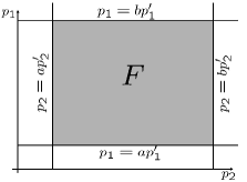
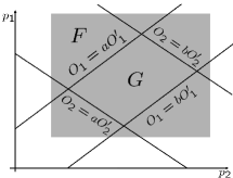
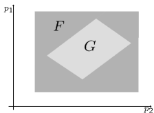
Figure 1: Left: In two dimensions the bounds placed on the parameters, $a\leq\frac{p_{i}}{p_{i}^{\prime}}\leq b$, appear as four lines in parameter space giving the dark grey area (2d volume), $F$. Middle: Bounds on the two observables, $a\leq\frac{O_{j}(\{p_{i}\})}{O_{j}(\{p_{i}^{\prime}\})}\leq b$ introduce four more lines which restrict $F$, giving the restricted subset, volume $G$. Right: Two dimensional volume (area) $F$ (dark grey) and the restricted subset, area $G$ (light grey).

As a first test of our measure we apply it to the Standard Model Hierarchy Problem. At one loop we can write, $m^{2}_{h}=m^{2}_{0}-C\Lambda^{2}$, where we treat $\Lambda^{2}$, the ultraviolet cutoff, and $m_{0}^{2}$, the bare mass, as the parameters. $C$ is a positive constant which includes gauge and Yukawa couplings.

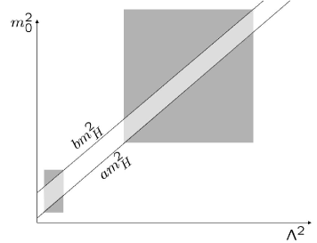
Figure 2: The two dimensional volume (area) $F$ (dark grey) and the restricted subset, area $G$ (light grey) for two different points in the two dimensional parameter space.

Varying these parameters about some point $P^{\prime}(m_{0}^{2},\lambda^{2})$ over the dimensionless interval $[a,b]$ defines an area, $F$ in the 2-d parameter space. Applying the same bounds to variations in the Higgs mass gives us two lines in the parameter space. Restricting $F$ to only allow such variations in the observables then defines our area $G$.

This is shown in Fig.(2) for two different points. For one, the values of the parameters are of the same order as the observable, $m_{h}^{2}$. Here G is not much smaller than $F$. The parameters of the other point are significantly larger than $m_{h}^{2}$. There $F$ is much larger than $G$, so this point is more tuned than the first. In general the areas are, $F=(b-a)^{2}m_{0}^{2}\Lambda^{2}$ and $G=(b-a)^{2}\Lambda^{2}m_{h}^{2}$, $\Rightarrow\triangle=\frac{F}{G}=1+\frac{C\Lambda^{2}}{m_{h}^{2}}=\triangle_{BG}$. In this simple case we find the same result as $\triangle_{BG}$.

In the MSSM there are many parameters, making analytical study difficult. Here we used a numerical version of our measure. We take random dimensionless fluctuations about a point, $P^{\prime}=\{p_{k}\}$, to get $N$ new points $\{P_{i}\}$. These are passed to a modified version of Softsusy 2.0.5Allanach:2001kg and each point $P_{i}$ is evolved from the GUT scale until electroweak symmetry is broken. An iterative procedure is used to predict $M_{Z}^{2}$ and then all the sparticle and Higgs masses are determined.

As before $F$ is the volume formed by dimensionless variations in the parameters. $G_{O_{i}}$ is the sub-volume of $F$ restricted to $a\leq\frac{O_{i}(\{p_{k}\})}{O_{i}(\{p_{k}^{\prime}\})}\leq b$ and $G$ is the sub-volume of $F$ restricted by $a\leq\frac{O_{j}(\{p_{k}\})}{O_{j}(\{p_{k}^{\prime}\})}\leq b$ for all observables $O_{j}$ predicted in Softsusy. For every $O_{i}$ a count ($N_{O_{i}}$) is kept of how often the point lies in the range $G_{O_{i}}$ as well as an overall count ($N_{O}$) of points are in $G$. Tuning is then measured using, $\triangle_{O_{i}}\approx\frac{N}{N_{O_{i}}}$, for individual observables and $\triangle\approx\frac{N}{N_{O}}$ for the overall tuning for that point.

We considered points on the MSUGRA benchmark slope sps1a Allanach:2002nj , defined by $m_{0}=-a_{0}=0.4m_{\frac{1}{2}}$, $sgn(\mu)=1$, $\tan{\beta}=10$. The benchmark point for this slope has $m_{0}=100{\rm GeV}$. Table 1 shows the tuning for $M_{Z}^{2}$ for two different ranges of variations in the parameters. Displayed first are tunings obtained by only allowing one parameter to vary, as for $\triangle_{BG}(p_{i})$. Results for R1 and R2 are the same, within statistical errors.

Also shown is our tuning measure for $M_{Z}^{2}$, where all parameters vary simultaneously. Here there is a $2\sigma$ deviation between results from R1 and R2. This could be a large statistical fluctuation or actual dependence on the range. However, for individual tunings, like $\triangle_{M_{Z}^{2}}$, a further complication may explain the deviation.

In particular, using Softsusy to predict the masses for the random points, sometimes we may have a tachyon, the Higgs potential unbounded from below, or non-perturbativity. Such points don’t belong in volume $G$ as they will give dramatically different physics. However it is unclear in which volumes, $G_{O_{i}}$ (significantly $G_{M_{Z}^{2}}$), the point lies. Such points never register as hits in any of the $G_{O_{i}}$ and this may artificially inflate the individual tunings, including $\triangle_{M_{Z}^{2}}$. Keeping the range as small as allowed by errors, minimises the number of problem points.

	$\triangle_{M_{Z}^{2}}(m_{\frac{1}{2}})$	$\triangle_{M_{Z}^{2}}(\mu)$	$\triangle_{M_{Z}^{2}}(y_{t})$	$\triangle_{M_{Z}^{2}}(ALL)$
$R1$	$38^{+4}_{-4}$	$41^{+5}_{-5}$	$25^{+2}_{-2}$	$56^{+4}_{-4}$
$R2$	$34^{+4}_{-3}$	$47^{+6}_{-5}$	$24^{+2}_{-2}$	$44^{+4}_{-4}$

Table 1: Tuning in $M_{Z}^{2}$ for sps1a. R1 and R2 are the dimensionless ranges $[\frac{1}{2},2]$ and $[0.9,1.1]$ respectively.

Next, using the smaller range, we applied our tuning measure for $M_{Z}^{2}$ to 12 more points on the sps1a slope. Moving along this slope in $m_{\frac{1}{2}}$ is an increase in the overall Susy breaking scale, since the magnitude of every soft breaking term is increasing. We have plotted the results of this investigation in Fig.(3).

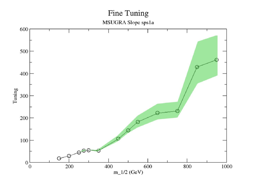
Figure 3: Tuning in $M_{Z}^{2}$ for sps1a slope. Statistical errors (one standard deviation) are shown by the shaded area about the plot.

As expected there is a clear increase in tuning as the Susy breaking scale is raised. The statistical error, shown by the shaded region, also increases with tuning, making the numerical approach most difficult to apply when tuning is large. However precise determinations of tuning are only relevant for moderate and low tunings. With tunings greater than $500$, precise values are not a likely requirement.

More work is needed before we can say anything definite about the overall tuning for the points here. We expect that the dominant tuning in the MSSM is $M_{Z}^{2}$, but nonetheless it will be interesting to see if there are any other significant contributions.

In summary the SM requires a tuning $\approx 10^{34}$ and this provides strong motivation for low energy supersymmetry. From searches at LEP it now appears that the MSSM may also be tuned, though only $\approx 10^{2}$. If true, rather than being a pathology, this may provide a hint for a GUT theory. Current measures of tuning cannot address this question, though, as they neglect the many parameter nature of fine tuning, ignore additional tunings in other observables, consider local stability only and assume ${\cal L}_{SUSY}$ is parametrised in the same way as ${\cal L}_{GUT}$. Here we have presented a new measure to address these issues. We have applied this measure, with uniform probability distributions, to the MSSM confirming that tuning in the $Z$ Boson mass increases with the Susy breaking scale.

References

- (1) R. Kitano and Y. Nomura, Phys. Lett. B 631, 58 (2005) [arXiv:hep-ph/0509039].
- (2) R. Barbieri and G. F. Giudice, Nucl. Phys. B 306, 63 (1988).
- (3) P. C. Schuster and N. Toro, arXiv:hep-ph/0512189.
- (4) B. C. Allanach, Comput. Phys. Commun. 143, 305 (2002) [arXiv:hep-ph/0104145].
- (5) B. C. Allanach et al., in Proc. of the APS/DPF/DPB Summer Study on the Future of Particle Physics (Snowmass 2001) ed. N. Graf, In the Proceedings of APS / DPF / DPB Summer Study on the Future of Particle Physics (Snowmass 2001), Snowmass, Colorado, 30 Jun - 21 Jul 2001, pp P125 [arXiv:hep-ph/0202233].
- (6) P. Athron and D. J. Miller, arXiv:0705.2241 [hep-ph].