Self-Similar Solutions of Viscous-Resistive ADAFs With Poloidal Magnetic Fields

Abstract

We carry out the self-similar solutions of viscous-resistive accretion flows around a magnetized compact object. We consider an axisymmetric, rotating, isotheral steady accretion flow which contains a poloidal magnetic field of the central star. The dominant mechanism of energy dissipation is assumed to be the turbulence viscosity and magnetic diffusivity due to magnetic field of the central star. We explore the effect of viscosity on a rotating disk in the presence of constant magnetic diffusivity. We show that the dynamical quantities of ADAFs are sensitive to the advection and viscosity parameters. Increase of the $\alpha$ coefficient in the $\alpha$-prescription model decreases the radial velocity and increases the density of the flow. It also affects the poloidal magnetic field considerably.

1 INTRODUCTION

Accretion onto black holes has been intensely studied for the last three decades (see Kato et al. 1998 for a review), and several types of models were proposed. Standard accretion disk model of Shakura $\&$ Sunyaev (1973) has been very useful in interpretation of observations in binary systems and active galactic nuclei, AGN (Pringle 1981), is based on a number of simplifying assumptions. In particular, the flow is assumed to be geometrically thin and with a Keplerian angular velocity distribution. This assumption allows gradient terms in the differential equations describing the flow to be neglected, reducing them to a set of algebraic equations and thereby fixes the angular momentum distribution of the flow. For low accretion rates, $\dot{M}$, this assumption is generally considered to be reasonable. Since the end of seventies, however, it has been realized that for high accretion rates, advection of energy with the flow can crucially modifies the properties of the innermost parts of accretion disks around black holes.

The natural improvement over the Shakura-Sunyeav model was to consider the case when cooling is less efficient than viscous heating. This may happen in two cases: either when the disk is extremely optically thick and the radiation is trapped for a timescale longer than the accretion timescale( see Abramowicz et al. 1988) or when it is extremely optically thin, a regime in which cooling processes are inefficient ( Narayan $\&$ Yi 1995b).

The study of advection accretion flows around low-luminosity black hole candidates and neutron stars are currently a very active field of research, both theoretically and observationally (see Narayan et al. 1998 for a review). Observational evidences for the existence of low luminosity black holes at the center of galaxies and in the active galactic nuclei AGN (Cherepashchuk 1996; Ho 1999) make necessary to revise theoretical models of the accretion disks. Thereby development of the subject of advection-dominated accretion flow (ADAF) in recent years lead to global solutions of advection accretion disks around accreting black hole systems and neutron stars. In this case, viscously generated internal energy is not radiated away efficiently as the gas falls into the potential well of the central mass (as in the standard thin disks model, Shakura & Sunyaev 1973) but retained within the accreting gas and advected radially inward (Narayan & Yi 1994, hereafter NY1994) and might eventually be lost into the central object or in contrast, a considerable portion of it might give rise to wind onto black holes and neutron stars (Blandford & Begelman 1999). By definition, Advection-Dominated Accretion Disks, ADAFs, have very low radiative efficiency as a consequence they can be considerably hotter than the gas flow in the standard thin disk models (Narayan & Yi 1995 a,b) and therefore they are ultra-dim for their accretion rates (Phinney 1981; Rees et al. 1982). On the other hand, since all the internal energy is stored as thermal energy, the gas becomes extremely hot and the kinetic temperature of ions approaches the virial limit what means that even at high initial angular momentum, the disk becomes very thick, forming practically a quasi-spherical accretion flow (Narayan & Yi 1995a). A general description of an advective accretion flow around a compact star was put forward by Narayan & Yi (1994, 1995a): they parameterized the degree of advection with one parameter $f$, defined as the ratio between the thermal energy stored in the disk and advected the central object ( not radiated), and the total thermal energy generated by viscosity at each radius. The general result obtained both from self-similar solutions and numerical calculations is that high advection $(f\sim 1)$ produces a hotter, thicker disk with a larger infall radial velocity and conversely a sub-Keplerian circular velocity.

A remarkable problem arises when the accretion disk was threaded by magnetic field. There are good reasons for believing that the magnetic fields are important in accretion processes in ADAFs. Some authors tried to study magnetized accretion flows analytically. For example ,Kaburaki (2000) presented a set of analytical solutions for a fully advective accretion flow in a global magnetic field. Shadmehri (2004), hereafter SH2004, extended this analysis by considering a non-constant resistivity. He obtained a set of self-similar solutions in spherical coordinates that described quasi-spherical magnetized accretion flow. The full account of the processes, connected with a presence of magnetic field in the flow, is changing considerably the picture of the accretion flow.

In ADAF models, energy dissipation in the accretion flow can be assumed to be due to turbulent viscosity and electrical resistivity. Under some conditions, it is important that we consider the effect of resistivity on accretion flows. Kuwabara et al. (2000) showed the results of global MHD simulations of an accretion flow initially threaded by large-scale poloidal magnetic fields including the effects of magnetic turbulent diffusivity. They found the importance of strength of magnetic diffusivity when they studied it in magnetically driven mass accretion. They pointed out that the mass outflow depends on the strength of magnetic diffusivity, so that for a highly diffusive disk, no outflow takes place. Thereby in this paper, we want to explore how the structure of a steady state thick disk depends on its resistivity and viscosity so we pursue SH2004’s work, resistive disks, when accretion flow experiences the rotation as well as viscosity dissipation. We consider ADAFs with the pure inflow and investigate the effect of viscosity on some physical quantities of the flows such as the radial and angular velocities, the density and the magnetic field flux. In order to study the dynamics of these flows, several simplified assumptions must be made in the analysis. The fluid is treated at least approximately as non-relativistic and also a poloidal model is adopted for electromagnetic field in which, it has a poloidal component in the disk. However, we will present self-similar solutions for viscous-resistive ADAFs.

This paper is organized as follows. Section 2, we present the equations of magnetohydrodynamics as the basic equations. General principles are presented in section 3. We show that the equations can be solved using the self-similar method and the numerical solutions are discussed in section 4 followed by results in section 5, summery and conclusion in section 6.

2 The Basic Equations

As we stated in introduction, we are interested in constructing a model for describing accretion disks in global magnetic fields. The macroscopic behavior of such flows can be studied by MHD equations. For simplicity the self-gravity of the disks and the effect of general relativity have been neglected. The flow is described in terms of the flow-frame time derivative or co-moving derivative, i.e. $\frac{D}{Dt}$ that defined as: $\frac{D}{Dt}=\frac{\partial}{\partial t}+(\textbf{u}\cdot\nabla)$. So, we can describe the accretion flows by the fundamental governing equations which are written by the equation of continuity:

$$\frac{D\rho}{Dt}+\rho{\nabla}\cdot\textbf{u}=0,$$ (1)

the equation of motion:

$$\rho\frac{D\textbf{u}}{Dt}=-{\nabla}p-\rho{\nabla}\Phi+\mu\nabla^{2}\textbf{u}+(\mu_{b}+\frac{1}{3}){\nabla}({\nabla}\cdot\textbf{u})+\frac{1}{4\pi}\textbf{J}\times\textbf{B},$$ (2)

the equation of energy:

$$\rho\left[\frac{D\epsilon}{Dt}+p\frac{D}{Dt}(\frac{1}{\rho})\right]=Q^{+}-Q^{-}=Q^{adv},$$ (3)

and the Maxwell‘s equations:

$${\nabla}\cdot\textbf{B}=0,$$ (4)

$$\frac{D\textbf{B}}{Dt}={\nabla}\times(\textbf{u}\times\textbf{B})+\eta\nabla^{2}\textbf{B},$$ (5)

where $\rho$ is the density of the gas, p the gas pressure, $\epsilon$ the internal energy, u the flow velocity, B the magnetic field, $\textbf{J}={\nabla}\times\textbf{B}$ the current density, $\eta$ the magnetic diffusivity in which for simplicity it is assumed to be a constant parameter (see, e.g., Kaburaki 2000), $\mu$ and $\mu_{b}$ are the shear and bulk viscosities, $Q^{adv}$ represents the advective transport of energy and is defined as the difference between the viscous heating rate $Q^{+}$ and radiative cooling rate $Q^{-}$. We neglect self-gravity so that $\Phi$ is assumed to be due to a central object. Also we neglect radiation pressure in the equations because in the optically thin ADAFs, $P^{gas}\gg P^{rad}$.

We employ the parameter $f=\frac{Q^{adv}}{Q^{+}}$(e.g., NY1994) to measure the degree to which the accretion flow is advection-dominated. In general, it will vary with r and depends on the details of the heating and cooling processes. For simplicity, it is assumed a constant. So, for advection-dominated flows we have $Q^{adv}\simeq Q^{+}\gg Q^{-}$. This corresponds to an optically thin ADAF where the viscous energy is stored in the gas as internal energy and the amount of cooling is negligible compared to the heating. In this case, the accreting gas has a very low density and accretion rates are low, sub-Eddington (Ichimaru 1977; Rees et al. 1982; NY1994; Abramowics et al. 1995). Correspondingly, for radiative-cooling-dominated flows we have $Q^{+}\simeq Q^{-}\gg Q^{adv}$. This corresponds to a cooling-dominated flow where the viscous energy is released in the gas as radiative energy and the amount of energy advected is negligible. The optically thick Shakura-Sunyaev disks correspond to this case.

Now, we formulate the basic equations (1)-(5) in spherical polar coordinates as follows:

$$\frac{\partial\rho}{\partial t}+\frac{1}{r^{2}}\frac{\partial}{\partial r}(r^{2}\rho u_{r})+\frac{1}{r}\frac{\partial}{\partial\theta}(\rho u_{\theta})=0,$$ (6)

The three components of the momentum equations give (e.g., Mihalas $\&$ Mihalas 1984):

$$\rho\left[\frac{\partial u_{r}}{\partial t}+u_{r}\frac{\partial u_{r}}{\partial r}+\frac{u_{\theta}}{r}\frac{\partial u_{r}}{\partial\theta}+\frac{u_{\phi}}{r\sin\theta}\frac{\partial u_{r}}{\partial\phi}-\frac{1}{r}(u_{\theta}^{2}+u_{\phi}^{2})\right]=-\frac{GM\rho}{r^{2}}-\frac{\partial p}{\partial r}$$ (7)

$$+\frac{\partial}{\partial r}\left[2\mu\frac{\partial u_{r}}{\partial r}+(\mu_{b}-\frac{2}{3}\mu)\left(\frac{1}{r^{2}}\frac{\partial}{\partial r}(r^{2}u_{r})+\frac{1}{r\sin\theta}\frac{\partial}{\partial\theta}(u_{\theta}\sin\theta)+\frac{1}{r\sin\theta}\frac{\partial u_{\phi}}{\partial\phi}\right)\right]$$

$$+\frac{1}{r}\frac{\partial}{\partial\theta}\left[r\mu\frac{\partial}{\partial r}\left(\frac{u_{\theta}}{r}\right)+\frac{\mu}{r}\frac{\partial u_{r}}{\partial\theta}\right]+\frac{1}{r\sin\theta}\frac{\partial}{\partial\phi}\left[\frac{\mu}{r\sin\theta}\frac{\partial u_{r}}{\partial\phi}+r\mu\frac{\partial}{\partial r}\left(\frac{u_{\phi}}{r}\right)\right]$$

$$+\frac{\mu}{r}\left[4r\frac{\partial}{\partial r}\left(\frac{u_{r}}{r}\right)-\frac{2}{r\sin\theta}\frac{\partial}{\partial\theta}(u_{\theta}\sin\theta)-\frac{2}{r\sin\theta}\ \frac{\partial u_{\phi}}{\partial\phi}+r\cot\theta\frac{\partial}{\partial r}\left(\frac{u_{\theta}}{r}\right)+\frac{\cot\theta}{r}\frac{\partial u_{r}}{\partial\theta}\right]$$

$$+\frac{1}{4\pi}\left\{-B_{\phi}\frac{1}{r}\frac{\partial}{\partial r}(rB_{\phi})-B_{\theta}\frac{1}{r}\left[\frac{\partial}{\partial r}(rB_{\theta})-\frac{\partial}{\partial\theta}B_{r}\right]\right\}$$

$$\rho\left[\frac{\partial u_{\theta}}{\partial t}+u_{r}\frac{\partial u_{\theta}}{\partial r}+\frac{u_{\theta}}{r}\frac{\partial u_{\theta}}{\partial\theta}+\frac{u_{\phi}}{r\sin\theta}\frac{\partial u_{\theta}}{\partial\phi}+\frac{1}{r}(u_{r}u_{\theta}-u_{\phi}^{2}\cot\theta)\right]$$ (8)

$$=-\frac{1}{r}\frac{\partial p}{\partial\theta}+\frac{1}{r}\frac{\partial}{\partial r}\left[r\mu\frac{\partial}{\partial r}\left(\frac{u_{\theta}}{r}\right)+\frac{\mu}{r}\frac{\partial u_{r}}{\partial\theta}\right]$$

$$+\frac{1}{r}\frac{\partial}{\partial\theta}\left[\frac{2\mu}{r}(\frac{\partial u_{\theta}}{\partial\theta}+(\mu_{b}-\frac{2}{3}\mu)\left(\frac{1}{r^{2}}\frac{\partial}{\partial r}(r^{2}u_{r})+\frac{1}{r\sin\theta}\frac{\partial}{\partial\theta}(u_{\theta}\sin\theta)+\frac{1}{r\sin\theta}\frac{\partial u_{\phi}}{\partial\phi}\right)\right]$$

$$+\frac{1}{r\sin\theta}\frac{\partial}{\partial\phi}\left[\frac{\mu\sin\theta}{r}\frac{\partial}{\partial\theta}\left(\frac{u_{\phi}}{\sin\theta}\right)+\frac{\mu}{r\sin\theta}\frac{\partial u_{\theta}}{\partial\phi}\right]$$

$$+\frac{\mu}{r}\left\{\frac{2\cot\theta}{r}\left[\sin\theta\frac{\partial}{\partial\theta}\left(\frac{u_{\theta}}{\sin\theta}\right)-\frac{1}{\sin\theta}\frac{\partial u_{\phi}}{\partial\phi}\right]+3r\frac{\partial}{\partial r}\left(\frac{u_{\theta}}{r}\right)+\frac{3}{r}\frac{\partial u_{r}}{\partial\theta}\right\}$$

$$+\frac{1}{4\pi}\left\{B_{r}\frac{1}{r}\left[\frac{\partial}{\partial r}(rB_{\theta})-\frac{\partial B_{r}}{\partial\theta}\right]-B_{\phi}\frac{1}{r\sin\theta}\frac{\partial}{\partial\theta}(B_{\phi}\sin\theta)\right\}$$

$$\rho\left[\frac{\partial u_{\phi}}{\partial t}+u_{r}\frac{\partial u_{\phi}}{\partial r}+\frac{u_{\theta}}{r}\frac{\partial u_{\phi}}{\partial\theta}+\frac{u_{\phi}}{r\sin\theta}\frac{\partial u_{\phi}}{\partial\phi}+\frac{u_{\phi}}{r}(u_{r}+u_{\theta}\cot\theta)\right]=-\frac{1}{r\sin\theta}\frac{\partial p}{\partial\phi}$$ (9)

$$+\frac{\partial}{\partial r}\left[\frac{\mu}{r\sin\theta}\frac{\partial u_{r}}{\partial\phi}+r\mu\frac{\partial}{\partial r}\left(\frac{u_{\phi}}{r}\right)\right]+\frac{1}{r}\frac{\partial}{\partial\theta}\left[\frac{\mu\sin\theta}{r}\frac{\partial}{\partial\theta}\left(\frac{u_{\phi}}{\sin\theta}\right)+r\mu\frac{\partial}{\partial r}\left(\frac{u_{\phi}}{r}\right)\right]$$

$$+\frac{1}{r\sin\theta}\frac{\partial}{\partial\phi}\left[\frac{2\mu}{r}\left(\frac{1}{\sin\theta}\frac{\partial u_{\phi}}{\partial\phi}+u_{r}+u_{\theta}\cot\theta\right)+(\mu_{b}-\frac{2}{3}\mu)\right.$$

$$\left.\times\left(\frac{1}{r^{2}}\frac{\partial}{\partial r}(r^{2}u_{r})+\frac{1}{r\sin\theta}\frac{\partial}{\partial\theta}(u_{\theta}\sin\theta)+\frac{1}{r\sin\theta}\frac{\partial u_{\phi}}{\partial\phi}\right)\right]$$

$$+\frac{1}{r\sin\theta}\frac{\partial}{\partial\phi}\left[\frac{\mu\sin\theta}{r}\frac{\partial}{\partial\theta}\left(\frac{u_{\phi}}{\sin\theta}\right)+\frac{\mu}{r\sin\theta}\frac{\partial u_{\theta}}{\partial\phi}\right]$$

$$+\frac{\mu}{r}\left\{2\cot\theta\left[\frac{\sin\theta}{r}\frac{\partial}{\partial\theta}\left(\frac{u_{\phi}}{\sin\theta}\right)+\frac{1}{\sin\theta}\frac{\partial u_{\theta}}{\partial\phi}\right]+3r\frac{\partial}{\partial r}\left(\frac{u_{\phi}}{r}\right)+\frac{3}{r\sin\theta}\frac{\partial u_{r}}{\partial\phi}\right\}$$

$$+\frac{1}{4\pi}\left\{B_{r}\frac{1}{r}\frac{\partial}{\partial r}(rB_{\phi})+B_{\theta}\frac{1}{r\sin\theta}\frac{\partial}{\partial\theta}(B_{\phi}\sin\theta)\right\}$$

while the equation of the energy gives:

$$\rho\left[\frac{\partial\epsilon}{\partial t}+u_{r}\frac{\partial\epsilon}{\partial r}+\frac{u_{\theta}}{r}\frac{\partial\epsilon}{\partial\theta}+\frac{u_{\phi}}{r\sin\theta}\frac{\partial\epsilon}{\partial\phi}-\frac{p}{\rho^{2}}\left(\frac{\partial}{\partial t}+u_{r}\frac{\partial}{\partial r}+\frac{u_{\theta}}{r}\frac{\partial}{\partial\theta}+\frac{u_{\phi}}{r\sin\theta}\frac{\partial}{\partial\phi}\right)\rho\right]$$ (10)

$$=2\mu f\left\{\left(\frac{\partial u_{r}}{\partial r}\right)^{2}+\frac{1}{r^{2}}\left(\frac{\partial u_{\theta}}{\partial\theta}+u_{r}\right)^{2}+\left[\frac{1}{r\sin\theta}\frac{\partial u_{\phi}}{\partial\phi}+\frac{1}{r}(u_{r}+u_{\theta}\cot\theta)\right]^{2}\right.$$

$$\left.+\frac{1}{2}\left[r\frac{\partial}{\partial r}\left(\frac{u_{\theta}}{r}\right)+\frac{1}{r}\frac{\partial u_{r}}{\partial\theta}\right]^{2}+\frac{1}{2}\left[r\frac{\partial}{\partial\phi}\left(\frac{u_{\phi}}{r}\right)+\frac{1}{r\sin\theta}\frac{\partial u_{r}}{\partial\phi}\right]^{2}\right.$$

$$\left.+\frac{1}{2}\left[\frac{\sin\theta}{r}\frac{\partial}{\partial\theta}\left(\frac{u_{\phi}}{\sin\theta}\right)+\frac{1}{r\sin\theta}\frac{\partial u_{\theta}}{\partial\phi}\right]^{2}\right\}$$

$$+f(\mu_{b}-\frac{2}{3}\mu)\left(\frac{1}{r^{2}}\frac{\partial}{\partial r}(r^{2}u_{r})+\frac{1}{r\sin\theta}\frac{\partial}{\partial\theta}(u_{\theta}\sin\theta)+\frac{1}{r\sin\theta}\frac{\partial u_{\phi}}{\partial\phi}\right)$$

also, the r-component of the induction equation

$$\frac{\partial B}{\partial t}=\frac{\partial}{\partial\theta}\left\{r\sin\theta\left[u_{\rm r}B_{\rm\theta}-\eta\frac{1}{r}\left(\frac{\partial}{\partial r}(rB_{\theta})-\frac{\partial B_{r}}{\partial\theta}\right)\right]\right\},$$ (11)

the $\theta$-component

$$\frac{\partial B}{\partial t}=\frac{\partial}{\partial r}\left\{r\sin\theta\left[u_{\rm r}B_{\rm\theta}-\eta\frac{1}{r}\left(\frac{\partial}{\partial r}(rB_{\theta})-\frac{\partial B_{r}}{\partial\theta}\right)\right]\right\},$$ (12)

the $\phi$-component

$$\frac{\partial B}{\partial t}=\frac{\partial}{\partial r}(ru_{\rm\varphi}B_{\rm r}-ru_{\rm r}B_{\rm\varphi})+\frac{\partial}{\partial\theta}(u_{\rm\varphi}B_{\rm\theta})+\frac{\partial}{\partial r}\left[\frac{\eta}{r}\frac{\partial}{\partial r}(rB_{\phi})\right]+\frac{\partial}{\partial\theta}\left[\frac{\eta}{r\sin\theta}\frac{\partial}{\partial\theta}(B_{\phi}\sin\theta)\right].$$ (13)

3 General Principles

As stated, we used a total of eight partial differential equations governing the non-self gravitating flow. These equations relate 15 dependent variables: $p,\rho,\epsilon,\mu,\mu_{b},\eta$ and the components of $\textbf{u},\textbf{J}$ and B. The equations must be closed by specifying suitable prescriptions for the viscosity and for the thermodynamics. Thus for the set of equations adopted, we make the following standard assumptions: we consider a steady ($\frac{\partial}{\partial t}=0$), rotating, axisymmetric ($\frac{\partial}{\partial\varphi}=0$), quasi spherical accreting flow (so it is convenient that we use spherical coordinates ($r,\theta,\phi$) in our discussion) with Keplerian angular velocity $\Omega_{k}(r)=(\frac{GM}{r^{3}})^{\frac{1}{2}}$ around a central object and with a purely poloidal magnetic field threading the disk. We assume that the fluid can be treated at least approximately as non-relativistic.

The kinematic viscosity coefficient, $\nu=\frac{\mu}{\rho}$, is generally parameterized using the $\alpha$-prescription (Shakura-Sunyaev 1973),

$$\nu=\alpha c_{s}H,$$ (14)

where $H=\frac{c_{s}}{\Omega_{k}}$ is known as the vertical scale height , $c_{s}=\sqrt{\frac{p}{\rho}}$ is the isothermal sound speed and the dimensionless coefficient $\alpha$ is assumed to be independent of r. Also it is important that we consider the effect of resistivity on accretion flows. So, we introduce the parameter $\eta$ as the magnetic diffusivity and insert it as a constant parameter in our equations. Both the kinematic viscosity coefficient $\nu$ and the magnetic diffusivity $\eta$ have the same units and are assumed to be due to turbulence in the accretion flow. Thus it is physically reasonable to express $\eta$ such as $\nu$ via the $\alpha$-prescription of Shakura-Sunyaev (1973) as follows (Bisnovatyi-Kogan & Ruzmaikin 1976),

$$\eta=\eta_{\circ}c_{s}H.$$ (15)

where the dimensionless coefficient $\eta_{\circ}$ is assumed independent of r. Bisnovatyi-Kogan and Ruzmaikin (1976) introduced $\eta_{\circ}$ and proposed that $\eta_{\circ}\sim\alpha$. Substituting $H$ and $c_{s}$ into the relations (14) and (15), we find them locally proportional to the pressure:

$$\nu=\alpha\frac{p}{\rho\Omega_{k}},$$ (16)

$$\eta=\eta_{\circ}\frac{p}{\rho\Omega_{k}}.$$ (17)

Their ratio is one definition of the magnetic Prandtl number as follows,

$$P_{m}=\frac{\nu}{\eta}=\frac{u_{T}\ell}{\eta}.$$ (18)

where $u_{T}$ is the random velocity of diffusing particle and $\ell$ is its mean free path. For a fully ionized hydrogen plasma Prandtl number is very large compared with unity due to the large length scale $\ell$ of the disk. In the following we consider conditions where $Pm\leq 1$. That means, viscous and resistive forces can be contributed in the energy dissipation similarly when it is equal to unity and resistive forces are dominate when $P_{m}$ is smaller than unity.

To determine thermodynamical properties of the flow in the energy equation (10), we require a constitutive relation as a function of two state variables. Therefore we choose an equation for the internal energy as $\epsilon=\frac{p}{\rho(\Gamma-1)}$ where $\Gamma$ is the ratio of specific heats of the gas.

To satisfy $\nabla\cdot\textbf{B}=0$, we may introduce a convenient functional form for the magnetic field. Owning to the axisymmetry, the magnetic field can be written as

$$\textbf{B}=\textbf{B}_{p}(r,\theta)+B_{\phi}(r,\theta)\textbf{e}_{\phi}$$ (19)

The effect of magnetic diffusivity on magnetically driven mass accretion was studied by Kuwabara et al. (2000). They showed that the effects of resistivity are that magnetic field lines do not rotate with the same angular speed as the disk matter and thus it suppresses the injection of magnetic helicity and magneto-centrifugal acceleration. So, neglecting the toroidal component of field, $B_{\phi}$, we can express the poloidal component, $\textbf{B}_{p}$, in terms of a magnetic flux function $\Psi(r,\theta)$:

$$\textbf{B}=\textbf{B}_{p}(r,\theta)=\frac{1}{2\pi}\nabla\times\left(\frac{\Psi}{r\sin\theta}\textbf{e}_{\phi}\right),$$ (20)

in which satisfies $\nabla\cdot\textbf{B}=\nabla\cdot\textbf{B}_{p}=0$. Magnetic flux function $\Psi(r,\theta)$ is related to the magnetic vector potential by $\Psi=rA_{\phi}$ with $A_{\phi}$ the toroidal component of the vector potential. The magnetic flux contained inside the circle $\rm r$=constant, $\theta=$constant is,

$$\int_{0}^{r}B_{\theta}(r^{\prime},\theta)2\pi r^{\prime}dr^{\prime}=2\pi\Psi(r,\theta)~{}~{}~{}~{}(+constant),$$ (21)

Since $B_{p}\cdot\nabla\Psi=0$, $\Psi$ labels magnetic lines or their surfaces of revolution, magnetic surfaces.

Similarity, one can write the flow velocity in the form

$$\textbf{u}=\textbf{u}_{p}(r,\theta)+u_{\phi}(r,\theta)\textbf{e}_{\phi},$$ (22)

subsequently, we show that the poloidal component of velocity has only a radial component $u_{p}=u_{r}$. We take $u_{r}$ to be a negative, since we want to consider infall of material.

It is clear that the basic equations are nonlinear and we cannot solve them analytically. Therefore, it is useful to have a simple means to investigate the properties of solutions. This is most easily done in terms of a set of dimensionless parameters which can be expected to be similar at all times. Here, one can employ the method of self-similar to fluid equations.

4 Self-Similar Solutions

To better understanding the the physical processes of our viscous-resistive ADAF accretion disks, we seek self-similar solutions of the above equations. The self-similar method is familiar from its wide applications to the full set of MHD equations. As long as we are not interested in boundaries of the problem, such solutions can accurately describe the behavior of the solutions in an intermediate region far from the radial boundaries.

Writing the equations in non-dimensional forms, that is, scaling all the physical variables by their typical values, brings out the non-dimensional variables. We can simply show that a solution of the following forms, satisfy the equations of our model:

$$\rho(r,\theta)=\rho_{\circ}\rho(\theta)(r/r_{\circ})^{-3/2},$$ (23)

$$\ p(r,\theta)=p_{\circ}P(\theta)(r/r_{\circ})^{-5/2},$$ (24)

$$\ u_{\rm r}(r,\theta)=r\Omega_{\rm K}(r)U(\theta),$$ (25)

$$\ u_{\rm\varphi}(r,\theta)=r\sin\theta\Omega_{\rm K}(r)\Omega(\theta),$$ (26)

$$\ B_{\rm r}(r,\theta)=\frac{B_{\circ}}{2\pi\sin\theta}\frac{d\Psi(\theta)}{d\theta}(r/r_{\circ})^{-5/4},$$ (27)

$$\ B_{\rm\theta}(r,\theta)=-\frac{3B_{\circ}\Psi(\theta)}{8\pi\sin\theta}(r/r_{\circ})^{-5/4}.$$ (28)

where $\rho_{\circ}$, $p_{\circ}$, $B_{\circ}$ and $r_{\circ}$ provide a non-dimensional form for our equations. Also $u_{\theta}=0$ is considered, since the most important assumption we made is that the flow is steady ($\frac{\partial}{\partial t}=0$) and also with respect to above solutions we find $r^{2}\rho u_{r}$ is independent of r but it is a function of $\theta$). It represents mass accretion rate in a given $\theta$. If we integrate this over the angle $\theta$, we obtain the net mass accretion rate

$$\dot{M}=-2{\dot{M}}_{\circ}\int\rho U\sin\theta d\theta$$ (29)

where ${\dot{M}}_{\circ}=2\pi\rho_{\circ}r^{2}_{\circ}\sqrt{\frac{GM}{r_{\circ}}}$.

We adopt $\alpha$-prescription (16) so that $\mu=\nu\rho=\alpha\frac{p}{\Omega_{k}}$. The bulk viscosity is not usually discussed in the context of accretion flows. Thus we assume $\mu_{b}=0$. Substituting the above solutions in the equations (7)-(13), we obtain a set of coupled ordinary differential equations in terms of $\theta$ for the three components of the equation of motion:

$$\rho\left(1-\frac{U^{2}}{2}-\Omega^{2}\sin^{2}\theta\right)= C_{\rm 1}P\left(2.5-\alpha U+\alpha\frac{dU}{d\theta}\cot\theta\right)$$ (30)

$$+\alpha C_{\rm 1}\frac{d}{d\theta}\left(P\frac{dU}{d\theta}\right)$$

$$+\frac{3C_{\rm 1}\Psi}{64\pi^{3}\sin\theta}\left[\frac{3\Psi}{16\sin\theta}-\frac{d}{d\theta}\left(\frac{1}{\sin\theta}\frac{d\Psi}{d\theta}\right)\right],$$

$$-\rho\Omega^{2}\sin\theta\cos\theta= -C_{\rm 1}\frac{dP}{d\theta}+\frac{\alpha}{2}C_{\rm 1}P\frac{dU}{d\theta}+\alpha C_{\rm 1}\frac{d}{d\theta}(PU)$$

$$+\frac{C_{\rm 2}}{16\pi^{3}\sin\theta}\frac{d\Psi}{d\theta}\left[\frac{3\Psi}{16\sin\theta}-\frac{d}{d\theta}\left(\frac{1}{\sin\theta}\frac{d\Psi}{d\theta}\right)\right],$$

$$\frac{1}{2}\rho U\Omega\sin\theta= -\frac{3}{4}\alpha C_{\rm 1}P\Omega\sin\theta+\alpha C_{\rm 1}\frac{d}{d\theta}\left(P\sin\theta\frac{d\Omega}{d\theta}\right)$$ (32)

$$+2\alpha C_{\rm 1}P\frac{d\Omega}{d\theta}\cos\theta,$$

the energy equation becomes:

$$\rho U\frac{3\Gamma-5}{2(\Gamma-1)}= \alpha\rho f\left[3U^{2}+\left(\frac{dU}{d\theta}\right)^{2}+\frac{9}{4}\Omega^{2}\sin\theta^{2}+\left(\frac{d\Omega}{d\theta}\right)^{2}\sin^{2}\theta\right]$$ (33)

$$+\frac{f\eta_{\rm 0}C_{\rm 2}}{16\pi^{3}}\left[\frac{3\Psi}{16\sin\theta}-\frac{d}{d\theta}\left(\frac{1}{\sin\theta}\frac{d\Psi}{d\theta}\right)\right]^{2},$$

equations (11) and (12) give:

$$-\rho\frac{d}{d\theta}(\Omega\Psi)-\rho\Omega\frac{d\Psi}{d\theta}=0,$$ (34)

the equation (13) gives:

$$-\frac{3\rho U\Psi}{4\eta_{\rm 0}C_{\rm 1}P\sin\theta}=\frac{3\Psi}{16\sin\theta}-\frac{d}{d\theta}\left(\frac{1}{sin\theta}\frac{d\Psi}{d\theta}\right).$$ (35)

where $C_{\rm 1}=\frac{p_{\circ}}{\rho_{\circ}}\left(\frac{GM}{r_{\circ}}\right)^{-1}=\frac{2p_{\circ}}{\rho_{\circ}u^{2}_{ff}}$ and $C_{\rm 2}=\frac{B^{2}_{\circ}}{\rho_{\circ}}\left(\frac{GM}{r_{\circ}}\right)^{-1}$.

The above equations constitute a set of ordinary differential equations for functions $U(\theta)$, $\Psi(\theta)$, $P(\theta)$ and $\Omega(\theta)$ as follows:

$$\frac{d^{2}U}{d\theta^{2}}= -\frac{2.5}{\alpha}+U-\frac{dU}{d\theta}\cot\theta-\frac{1}{P}\frac{dP}{d\theta}\frac{dU}{d\theta}$$ (36)

$$+\frac{\rho}{\alpha C_{\rm 1}P}(1-\frac{U^{2}}{2}-\Omega^{2}\sin^{2}\theta)+\frac{2U\rho}{\beta_{\circ}\eta_{\circ}\alpha C_{\rm 1}}\left(\frac{3\Psi}{8\pi P\sin\theta}\right)^{2},$$

$$\frac{d^{2}\Psi}{d\theta^{2}}=\frac{d\Psi}{d\theta}\cot\theta+\left(\frac{3}{16}+\frac{3U\rho}{4\eta_{\circ}C_{\rm 1}P}\right)\Psi,$$ (37)

$$\frac{d^{2}\Omega}{d\theta^{2}}=\frac{\rho U\Omega}{2\alpha C_{\rm 1}P}+\frac{3}{4}\Omega-3\frac{d\Omega}{d\theta}cot\theta-\frac{1}{P}\frac{dP}{d\theta}\frac{d\Omega}{d\theta},$$ (38)

$$\frac{dP}{d\theta}=\frac{3\alpha P}{2(1-\alpha U)}\frac{dU}{d\theta}-\frac{3\rho U\Psi}{8\pi^{2}\beta_{\circ}\eta_{\circ}C_{\rm 1}P\sin^{2}\theta(1-\alpha U)}\frac{d\Psi}{d\theta},$$ (39)

$$\frac{d\Omega}{d\theta}=-\frac{2\Omega}{\Psi}\frac{d\Psi}{d\theta}.$$ (40)

where $\beta_{\circ}=\frac{P_{\circ}}{B^{2}_{\circ}/8\pi}$. Integrating the last equation, and doing some simplifications we have $\Omega\Psi^{2}=K$, where $K$ is an arbitrary constant. Also we can obtain $\rho$ as follows,

$$\rho=-\frac{\beta_{\circ}\eta_{\circ}C_{\rm 1}}{2}\left(\frac{8\pi P\sin\theta}{3U\Psi}\right)^{2}\left[\frac{1.5(5-3\Gamma)U}{3f(\Gamma-1)}+3\alpha U^{2}\right.$$

$$\left.+\alpha(\frac{dU}{d\theta})^{2}+\frac{9}{4}\alpha\Omega^{2}\sin^{2}\theta+\alpha\sin^{2}\theta(\frac{d\Omega}{d\theta})^{2}\right].$$ (41)

From equation (40) we can find:

$$\frac{d^{2}\Psi}{d\theta^{2}}=\frac{3}{4}\frac{\Psi}{\Omega^{2}}(\frac{d\Omega}{d\theta})^{2}-\frac{\Psi}{2\Omega}(\frac{d^{2}\Omega}{d\theta})^{2}\\$$ (42)

Comparing equations (37) and (42) we can eliminate $\Psi$ and then the result can be compared with equation (38), finally we have:

$$3(\frac{d\Omega}{d\theta})^{2}+2A\frac{d\Omega}{d\theta}-B=0,$$ (43)

where

$$A=\frac{\Omega}{P}\frac{dP}{d\theta}+4\Omega\cot\theta,$$

$$B=\left[\frac{9}{4}+(\frac{1}{\alpha}+\frac{3}{\eta_{0}})\frac{\rho U}{c_{1}P}\right]\Omega^{2},$$

Equation (43) is an ordinary first order differential equation for $\Omega^{{}^{\prime}}=\frac{d\Omega}{d\theta}$, and it has two roots:

$$\Omega^{{}^{\prime}}=\frac{-A\pm\sqrt{{A^{2}+3B}}}{3}$$ (44)

substituting the above solution in the main equations of the system, (36)-(37)-(39), and eliminating $\Psi$ we obtain:

$$\frac{dP}{d\theta}= \frac{3\alpha P}{2(1-\alpha U)}\frac{dU}{d\theta}+\frac{3\rho KU}{16\pi^{2}\beta_{0}\eta_{0}C_{1}P\Omega^{2}\sin^{2}\theta(1-\alpha U)}\frac{d\Omega}{d\theta}+\frac{\rho\Omega^{2}\sin\theta\cos\theta}{C_{1}(1-\alpha U)}$$ (45)

$$\frac{d^{2}U}{d^{2}\theta}= -\frac{2.5}{\alpha}+U-\cot\theta\frac{dU}{d\theta}-\frac{1}{P}\frac{dP}{d\theta}\frac{dU}{d\theta}+\frac{\rho}{C_{1}\alpha P}(1-\frac{U^{2}}{2}-\Omega^{2}\sin^{2}\theta)$$ (46)

$$+\frac{2UK\rho}{\beta_{0}\eta_{0}\alpha C_{1}\Omega}(\frac{3}{8\pi\rho\sin\theta})$$

$$\rho= -\frac{\beta_{0}\eta_{0}C_{1}}{2}(\frac{8\pi P\sin\theta\Omega^{\frac{1}{2}}}{3UK^{\frac{1}{2}}})^{2}\left[\frac{1.5(5-3\Gamma)}{3f(\Gamma-1)}+3\alpha U^{2}+\alpha\frac{dU}{d\theta}+\frac{9}{4}\alpha\Omega^{2}\sin^{2}\theta\right.$$ (47)

$$\left.+\alpha\sin^{2}\theta(\frac{d\Omega}{d\theta})^{2}\right]$$

Equations (44)-(47) constitute a system of ordinary non-linear differential equations for the four self-similar variables, $\Omega,P,U,\rho$. Indeed, the behavior of the solutions depends on boundary conditions which are supposed based on some physical assumptions such as symmetry with respect to the equatorial plane, etc.

There are many techniques for solving these nonlinear equations. Analytical methods can yield solutions for some simplified problems. But, in general this approach is too restrictive and we have to use the numerical methods. Here, one can employ the method of relaxation to the fluid equations (Press et al. 1992). In this method we replace ordinary differential equations by approximate finite-difference equations on a grid of points that spans the domain of interest. The relaxation method determines the solution by starting with a guess and improving it, iteratively. Based on it, this system of equations can be solved for all unknowns as a function of $\theta$, once if we have a complete set of boundary conditions which put some physical constraints on the flow. The boundary conditions are distributed between the equatorial plane, $\theta=\frac{\pi}{2}$ and the rotation axis, $\theta=0$. The boundary conditions at $\theta=0$ are:

$$\frac{dU}{d\theta}=\frac{d\Omega}{d\theta}=\frac{dP}{d\theta}=\frac{d\Psi}{d\theta}=0~{}~{}~{},~{}~{}~{}U=0,$$ (48)

and in this method the boundary conditions at $\theta=\frac{\pi}{2}$ are:

$$\frac{dU}{d\theta}=\frac{d\Omega}{d\theta}=\frac{dP}{d\theta}=\frac{d\Psi}{d\theta}=0.,$$ (49)

We have found condition $\frac{d\Psi}{d\theta}=0$ by the relation $\Omega\Psi^{2}=K$ for both two boundaries which demand the magnetic flux enclose by the polar axis goes to zero. So field line thread the equator vertically. We have a limitation to reach $\theta=0$ numerically. So we try to use boundary condition very close to polar axis with very small value of $\theta$. We can obtain physical solutions if we consider the big value of $\Omega$ and so $\Psi\simeq 0$ at $\theta=\epsilon$. Also, at $\theta=\frac{\pi}{2}$ the equations (44) and (47) gives:

$$\rho=\frac{P}{U}\delta,$$

$$U\delta=\gamma P\left[\frac{3}{2}\epsilon^{{}^{\prime}}+3\alpha U^{2}+\frac{9}{4}\alpha\right],$$

where

$$\epsilon^{{}^{\prime}}=\frac{3(5-\Gamma)}{2f(\Gamma-1)},~{}~{}~{}~{}~{}\delta=-\frac{9\alpha C_{1}\eta_{0}}{4(\eta_{0}+3\alpha)},~{}~{}~{}\gamma=-\frac{32\beta_{0}\eta_{0}C_{1}\pi^{2}}{9K},$$

The boundary conditions on the above equations require that variables are assumed to be regular at the endpoints. Also the net mass accretion rate (29) provides one boundary condition for $\rho$:

$$\int_{0}^{\frac{\pi}{2}}\rho(\theta)U(\theta)\sin\theta d\theta=-\frac{1}{2},$$

For solving the MHD equations numerically, we need these boundary conditions. Using these boundary conditions require to choose $K,\epsilon^{{}^{\prime}},\delta,\gamma$ properly. So we are going to have a astrophysical approximations for this variables.

For our illustrative parameters, we consider approximate equipartition of magnetic and kinetic energies for matter flowing into a neutron star. In quasi-spherical accretion flows, approximate equipartition proposed by Shwartsman (1971),

$$\frac{B^{2}}{8\pi}\simeq\frac{1}{2}\rho u_{r}^{2},$$ (50)

where $u_{r}$ corresponds to an Alfv́en speed $u_{A}=\frac{B}{\sqrt{4\pi\rho}}\simeq u_{\rm{ff}}$ (free-fall speed). The density of the infalling materials can be reasonably approximated by free-fall behavior. In the accretion disks around the magnetized compact object, due to the complicated nonlinear effects from the interaction between accretion materials and the magnetic fields of the compact object, the mechanisms that led to the magnetic field chandeled accretion flow still remain unsolved. However, it is widely accepted that due to strong gravity of the compact object, a very steep and supersonic flow hits the magnetosphere boundary and deforms its structure drastically. The infalling flow is halted at distance $r\sim r_{A}$ where the magnetic energy density balances the flow kinetic energy, or $u_{A}=u_{\rm{ff}}$. Here $u_{A}$ is calculated from free fall density and velocity:

$$\rho_{\rm{ff}}=\frac{\dot{M}}{4\pi r_{\rm A}^{2}u_{\rm ff}},~{}~{}~{}~{}~{}~{}~{}~{}~{}~{}~{}u_{\rm{ff}}=\sqrt{\frac{2GM}{r}}$$ (51)

where $\dot{M}$ is the mass accretion rate and $r_{A}$ Alfv́en radius. Interestingly, the numerical simulations (Paatz $\&$ Camenzind 1996, Koldoba, Lovlace $\&$ Ustyugova 2002) show that at this distance $r\sim r_{A}$ the material funnels through the magnetosphere and fall onto the magnetic poles. The funnel flow is found to reach the star’s magnetic poles with the velocity close to that of free-fall velocity.

The magnetic configuration outside of a compact star, such a neutron star, is a dipole field then in spherical polar coordinates we have

$$\textbf{B}=B_{p}R^{3}\left(\frac{2\cos\theta}{r^{3}}\textbf{e}_{r}+\frac{\sin\theta}{r^{3}}\textbf{e}_{\theta}\right)$$ (52)

where R is the radius of the neutron star and $B_{p}$ is the magnetic field at the magnetic poles. Thus in the equatorial plane ($\theta=\frac{\pi}{2}$), the equation (52) becomes $B\simeq\frac{B_{p}R^{3}}{r^{3}}$. So we obtain,

$$\frac{\dot{M}}{4\pi r_{\rm A}^{2}u_{ff}}\simeq\frac{B^{2}_{p}R^{6}}{8\pi GMr_{\rm A}^{5}}.$$ (53)

The equation (53) implies that the infalling mass close to the equatorial plane of a neutron star is stopped at a radial distance,

$$r_{\rm A}=B_{p}^{4/7}R^{12/7}{\dot{M}}^{-2/7}(2GM)^{-1/7}$$ (54)

for $M\sim M_{\odot}$, ${\dot{M}}\sim 1.85\times 10^{16}gs^{-1}(\dot{M}<\dot{M}_{Edd}=1.39\times 10^{18}\frac{M}{M\odot}gs^{-1})$, $B_{p}\sim 10^{12}G$ and $R\sim 10^{6}cm$, the equation (54) gives $r_{\circ}\sim r_{\rm A}\sim 5.2\times 10^{8}cm$. Thus we can obtain $B_{\circ}=B_{p}\left(\frac{R}{r_{\circ}}\right)^{3}\sim 10^{6}G$ and $\rho_{\circ}\sim 3.6\times 10^{-10}g~{}{cm}^{-3}$. On the other hand, the gas pressure, density and temperature are related by

$$p_{\circ}=\frac{\rho_{\circ}kT}{\mu_{\circ}m_{H}}$$ (55)

where $\mu_{\circ}$ is the mean molecular weight, k Boltzman constant and $m_{H}\sim m_{p}$ is the mass of the hydrogen atom. We assume the accreting materials to be mainly hydrogen and to be nearly ionized. For accreted materials, the potential energy released is $\frac{GM_{*}M_{acc}}{r_{\circ}}$ and the thermal energy is $2\times\frac{3}{2}kT$ ($T_{\rm vir}=\frac{T_{\rm th}}{2}$); therefore, $T_{th}=\frac{GM_{*}M_{\rm acc}}{3kr_{\circ}}\sim 5.5\times 10^{9}K$ we obtain $p_{\circ}\sim 3.2\times 10^{8}dyne~{}cm^{-2}$. Consequently, in turn it can be reduced that $\beta_{\circ}=0.01$, $C_{1}=0.8$ and $C_{2}=2\times 10^{3}$.

Imposing two boundary conditions (48) and (49) to the equations (44)-(47), we obtain numerical solutions for the flows with a fixed value of $\eta_{\circ}=0.1$, $\Gamma=4/3$ and $\alpha=0.01,0.05$ and $0.1$ with a sequence of the increasing values of parameter f or decreasing cooling. Figures 1-5 show our results.

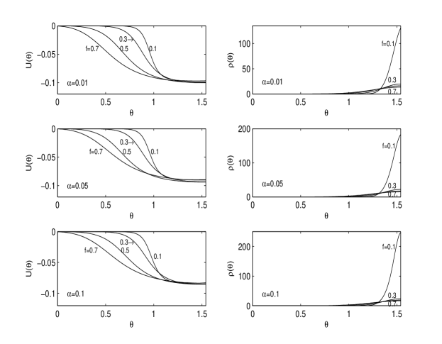
Figure 1: The self-similar solutions of radial velocity $U$ (left panels) and density $\rho$ (right panels) as a function of polar angel $\theta$ corresponding to for Top: $\alpha$=0.01, Middle: $\alpha$=0.05 and Bottom: $\alpha$=0.1.

5 Results: Typical Solutions

We have obtained numerical solutions of equations (44)-(47) for variety of values of the viscosity parameter $\alpha$ and advection parameter $f$. Figures 1-4 show a typical sequence of solutions correspond to $\alpha=0.01,0.05,0.1$ and $f=0.1,0.3,0.5,0.7$. The solutions may be considered either as flows with a fixed value of viscosity parameter and with a sequence of increasing advection parameter or decreasing cooling (Figures 1 and 3) or a sequence of different values of viscosity parameter $\alpha$ in a fixed advection regime (Figures 2 and 4).

The six panels in Figure 1 show the variations with respect to the polar angle $\theta$ of various dynamical quantities in the solutions. The top left panel displays the dimensionless radial velocity $U(\theta)$ as a function of $\theta$. The velocity is zero at $\theta=0$ (this is a boundary condition) and maximum at $\theta=\frac{\pi}{2}$. So the maximum accretion velocity is at equatorial region and on the polar axis there is no mass inflow. As we expected the velocity is sub-Keplerian. We find that in the boundary, $U(\theta)$ is essentially independent of advection parameter $f$. But in the intermediate, the radial velocity is modified by $f$; in the SH2004 solutions, two distinct regions in the $U(\theta)$ profile could be recognized. The bulk of accretion occurs from equatorial plane at $\theta=\frac{\pi}{2}$ to a surface at $\theta=\theta_{s}$, inside of which the radial velocity is zero. While NY1994 solutions there is no zero inflow in $0<\theta<\frac{\pi}{2}$. Our solutions show that in a given $\theta$ the radial velocity is increased when we increase the advection parameter. The middle and bottom left panels display the radial velocity in $\alpha=0.05,0.1$ for a sequence of advection parameters respectively.

The top right panel shows profile of the density $\rho(\theta)$. The density contrast in the equatorial and polar regions increase with decreasing advection parameter $f$. The density grows and becomes concentrated toward the equatorial plane. For a given $\alpha$, solutions with small values of $f$ behave like standard thin disks, as might be expected since these solutions correspond to $f\rightarrow 0$ and so advect very little energy. In the opposite advection-dominated limit, which corresponds to $f\rightarrow 1$, our solutions describe nearly spherical flows which rotate at much below the Keplerian velocity. This is demonstrated in Figure 5 where we display iso-density contours in the meridional plane. The middle and bottom right panels display the density profiles in $\alpha=0.05,0.1$ for a sequence of advection parameters respectively. This advection-dominated solutions have very similar properties to the approximated solutions derived by NY1994 and SH2004. The results show that these quantities are very sensitive to the advection parameter. For low advection regimes, $f=0.1,0.3$, we have to separate the regime for radial inflow. But for high advection regimes $f=0.5,0.7$, the radial velocity is non zero around the pole.

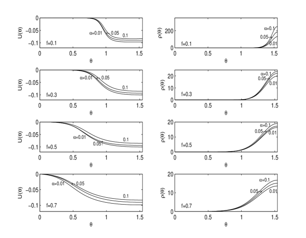
Figure 2: The self-similar solutions of radial velocity $U$ (left panels) and density $\rho$ (right panels) as a function of polar angel $\theta$ corresponding to $\Gamma=4/3$, $\eta_{0}=0.1$, $\beta_{0}=0.01$ and $\alpha=0.01,0.05,0.1$ for $f=0.1,0.3,0.5,0.7$ from Top to Bottom, respectively.

The behavior of the solutions, self-similar radial velocity and density profile, are demonstrated in Figure 2 for different values of advection parameters with variation of viscosity parameters. The panels in Figure 2 show that For a fixed $f$, the density maximum increases with increasing viscosity parameter while the radial velocity decreases with increasing it. In this case, increasing the viscosity parameter corresponds to increasing heating mechanisms, so in a fixed advection regime, there are more energy to advect into central star. The top Panels in Figure 5 Show that the disk to be thick. The solution with the same $f$ but with different values of $\alpha$ are virtually indistinguishable from one another. There are probably, more significantly variations when $\alpha$ exceeds above $0.1$. Recently King et al. 2007 assart that in a thin and fully ionized disk the best observational evidence suggest a typical range $\alpha\sim 0.1-0.4$ where relevant numerical simulations tend to drive estimates for $\alpha$ which are an order of magnitude smaller. However, such large values of $\alpha$ are probably unlikely (eg. Narayan, Loab, $\&$ Kumar 1994; Hawley, Gammie, $\&$ Balbus 1994), and so we have not explored this region of the $\alpha$ parameter.

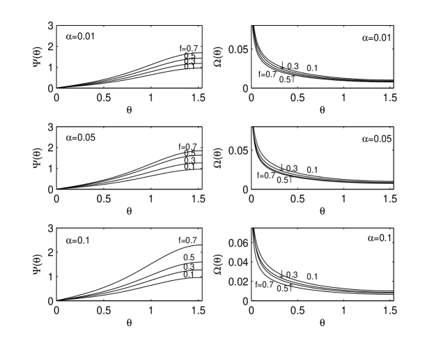
Figure 3: The self-similar solutions of magnetic flux $\Psi$ (left panels) and angular momentum $\Omega$ (right panels) as a function of polar angel $\theta$ corresponding to $\Gamma=4/3$, $\eta_{0}=0.1$, $\beta_{0}=0.01$, $f=0.1,0.3,0.5,0.7$ for Top: $\alpha$=0.01, Middle: $\alpha$=0.05 and Bottom: $\alpha$=0.1 in rotating accretion flows.

The $U(\theta)$ and $\rho(\theta)$ profiles both peak at $\theta=\frac{\pi}{2}$. Therefore, in all our solutions the bulk of accretion occurs along the equatorial plane and accretion rate goes to zero along the rotational pole. An interesting feature of these solutions, as already mentioned, for low advection ,$f$, we have a thin disk; in all cases there is a low density with a higher temperature corona above the disk.

Figure 3 displays the magnetic flux function and the angular velocity for different values of advection parameter in a fixed viscosity parameter. Integration of equation (40) yields $\Omega\Psi^{2}=K$, where $K$ is an arbitrary constant. So angular velocity and magnetic flux function should have opposite behavior along $\theta$ direction. We plot them with choosing proper input parameters which introduced in the end of the last section. Figure 3 shows that magnetic flux function, $\Psi(\theta)$, varies by only $\sim 50$ percent. The magnetic flux function increases by increasing advection in accretion disk in a fixed viscosity. The behavior of angular velocity is exactly opposite. Figure 4 displays the behavior of the magnetic flux and angular velocity for different values of viscosity parameter in a fixed advection. The solutions implies that in a fixed, low $f$, the effect of different $\alpha$ is indistinguishable.

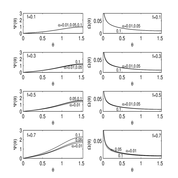
Figure 4: The self-similar solutions of magnetic flux $\Psi$ and angular momentum $\Omega$ as a function of polar angel $\theta$ corresponding to $\Gamma=4/3$, $\eta_{0}=0.1$, $\beta_{0}=0.01$ and $\alpha=0.01,0.05,0.1$ for $f=0.1,0.3,0.5,0.7$ from Top to Bottom, respectively.

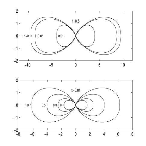
Figure 5: Isodensity contours in the meridional plane for $\Gamma=4/3$, $\eta_{0}=0.1$, $\beta_{0}=0.01$ for Top: $f$=0.5 and $\alpha$=0.01, 0.05, 0.1, Bottom: $\alpha$=0.01 and $f$=0.1, 0.3, 0.5, 0.7.

6 SUMMERY AND CONCLUSION

The main aim of this investigation was to obtain axisymmetric self-similar advection-dominated solution for viscose-resistive accretion flow. We have presented the results of self-similar solutions of the effect of the viscosity and rotation on magnetically driven accretion flows from a flow threaded by poloidal magnetic fields where only serious approximation we have made is the use of an isotropic $\alpha$ viscosity and constant magnetic diffusivity. Attention has restricted to flow accretions in which self-gravitation is negligible. We included the magnetic diffusivity so that its value was constant throughout our analysis. Using the basic equations of fluid dynamics in spherical polar coordinates $(r,\theta,\phi)$, we have employed the method of self-similar for thick discs to derive a set of coupled differential equations which govern the dynamics of the system. We then solved the equations by the method of relaxation by considering boundary conditions and using $\alpha$-prescription (Shakura & Sunyaev, 1973) in order to extract some of the similarity functions in terms of the polar angle $\theta$. Figures are considered for $\alpha=0.01,0.05,$ and $0.1$ so that for any $\alpha$ we considered $f=0.1,0.3,0.5$ and $0.7$.

We showed that the radial and rotational velocities are well below the Keplerian velocity. The Bulk of accretion with nearly constant velocity occur in the region which extend from equatorial plane to a given $\theta$ which highly depends on advection parameter $f$. In a non-advective regime, low $f$, we have a standard thin accretion disk but for high $f$ the accretion is nearly spherical. The geometrical shape of the flow is determined by the amount of viscosity and advection, in a fixed magnetic diffusivity. The accretion disk with efficient cooling ($f\rightarrow 0$) has low-density, high temperature corona which implies that the regular thin disks may be accompanied by advection-dominated corona which can drive low-density wind.

Our results show the flow of ionized accretion materials is not disklike in morphology. The closest along our solution in the accretion literature is Bondi (1952) spherical accretion. Our flows differ in important ways from Bondi problem. The gas in our model rotates and has viscose interaction through which angular momentum is transported outward. Also, our flow has magnetic interaction with dipole magnetic field of the central star which it can redistribute the angular momentum within the accretion disk. The angular velocity is significantly sub-Keplerian, and this may have an important role in spin-up of accreting stars. Stars which their spins grow by interacting with accretion materials are likely to reach a steady state with a rotation rate below the break-up limit. This advection-dominated solution may be a good solution for angular momentum problem in the star formation.

However, our results improve the physics of advection-dominated accretion disks. It is important that the magnetic diffusivity can modify the dynamical quantities of the disks. We developed NY1994 solutions to a realistic model for ADAFs by adding magnetic diffusivity. But in future we are going to investigate the effect of non-constant magnetic diffusivity, $\eta_{0}$. Several developments can be investigated to reach a much realistic description of the physics of accretion disks around the magnetized compact objects.

References

• (1) Abramowicz, M. A., Czerny, B., Lasota, J. P., & Szuszkiewicz, E. 1988, ApJ, 332, 646
• (2) Abramowicz, M. A., Chen, X., Lasota, J. P., & Regev, O. 1995, ApJ, 438, L37
• (3) Bisnovatyi-Kogan, G. S., & Ruzmaikin, A. A. 1976, Ap&SS, 42, 401
• (4) Blandford, R. D., & Begelman, M. C. 1999, MNRAS, 303, L1
• (5) Bondi, H., 1952, MNRAS, 112, 195
• (6) Cherepashchuk, A. M. 1996 Uspekhi Fiz. Nauk 166, 809
• (7) Hawley, J. F., Gammie, C. F., & Balbus, S. A., 1994, ASPC, 54, 73H
• (8) Ho, L. 1999, In: Proc. Conf. Observational Evidences for Black Holes in the Universe, Calcutta, 1998. Kluwer, P. 157
• (9) Ichimaru, S. 1977, ApJ, 214, 840
• (10) Kaburaki, O. 2000, ApJ, 531, 210
• (11) Kato, S., Fukue, J., & Mineshige, S. 1998, Black Hole accretion disks
• (12) King, A. R., Pringle, J. E., & Livio, M. 2007,Astro-ph:/0701803
• (13) Koldoba, A., V., Lovelace, R., V., E. & Ustyugova, A., V., 2002, AJ, 123, 2019
• (14) Kuwabara, T., Shibata, K., Kudoh, T., & Matsumoto, R. 2000, PASJ, 52, 1109
• (15) Mihalas,D., $\&$ Mihalas, B. W. 1984, Foundations of Radiation Hydrodynamics (New York: Oxford Univ. Press)
• (16) Narayan, R., Loab. A., & Kumar, P. 1994, ApJ, 431, 359
• (17) Narayan, R., & Yi, I. 1994, ApJ, 428, L13
• (18) Narayan, R., & Yi, I. 1995a, ApJ, 444, 238
• (19) Narayan, R., & Yi, I. 1995b, ApJ, 452, 710
• (20) Narayan, R., Mahadevan, R., & Quataert, E. 1998, in The Theory of Black Hole Accretion Disks, ed. M. A. Abramowicz, G. BjΓΆrnsson, & J. E. Pringle (Cambridge: Cambridge Univ. Press), 148
• (21) Paatz, G. & Camenzind, M., 1996, A&A, 308, 77
• (22) Phinney, E. S. 1981, in Plasma Astrophysics, ed. T. D. Guyenne & G. Lev (ESA SP-161), 337
• (23) Press, W. H., Teukolsky, S. A., Vetterling, W. T., & Flannery, B. P. 1992, Numerical Recipes.
• (24) Pringle, J. E. 1981, ARA&A, 19, 137p
• (25) Rees, M. J., Begelman, M. C., Blandford, R. D., & Phinney, E. S. 1982, Nat, 295, 17
• (26) Schwartzman, V. F. 1971, Soviet Astron, 15, 377
• (27) Shadmehri, M. 2004, A&A, 424, 379
• (28) Shakura, N. I., & Sunyaev, R.A. 1973, A&A, 24, 337