UNSTABLE DISK GALAXIES. I. MODAL PROPERTIES

Abstract

I utilize the Petrov-Galerkin formulation and develop a new method for solving the unsteady collisionless Boltzmann equation in both the linear and nonlinear regimes. In the first order approximation, the method reduces to a linear eigenvalue problem which is solved using standard numerical methods. I apply the method to the dynamics of a model stellar disk which is embedded in the field of a soft-centered logarithmic potential. The outcome is the full spectrum of eigenfrequencies and their conjugate normal modes for prescribed azimuthal wavenumbers. The results show that the fundamental bar mode is isolated in the frequency space while spiral modes belong to discrete families that bifurcate from the continuous family of van Kampen modes. The population of spiral modes in the bifurcating family increases by cooling the disk and declines by increasing the fraction of dark to luminous matter. It is shown that the variety of unstable modes is controlled by the shape of the dark matter density profile.

1. INTRODUCTION

Dynamics of self-gravitating stellar systems and plasma fluids are governed by the collisionless Boltzmann equation (CBE) (Binney & Tremaine, 1987). Finding a general solution of the CBE has been a challenging problem in various disciplines of physical sciences. Due to existing difficulties of the general problem, finding a solution to the linearized CBE became the center of attraction in the twentieth century when Landau (1946) and van Kampen (1955) discovered the normal modes of collisionless ensembles. Later in 1970’s, Kalnajs (1971, 1977) developed a matrix theory that was capable of computing normal modes of stellar systems through solving a nonlinear eigenvalue problem. His theory remained as the only analytical perturbation theory used by the community of galactic dynamicists over the past three decades.

Kalnajs (1977) assumed an exponential form $\exp(-{\rm i}\omega t)$ for the time-dependent part of physical quantities where ${\rm i}=\sqrt{-1}$, and solved the linearized CBE for the perturbed distribution function (DF) $f_{1}$ in terms of the perturbed potential $V_{1}$. After expanding the potential and density functions in terms of bi-orthogonal basis sets in the configuration space, he used the weighted residual form of the fundamental equation

$$f_{1}d\textbf{{v}}d\textbf{{x}}=\Sigma_{1}d\textbf{{x}},$$ (1)

to obtain a nonlinear eigenvalue problem for the complex eigenfrequency $\omega$. For self-consistent perturbations the surface density $\Sigma_{1}=\int f_{1}d\textbf{{v}}$ is related to $V_{1}$ through Poisson’s integral, and the symbols $d\textbf{{v}}$ and $d\textbf{{x}}$ denote the elements of velocity and position vectors.

Zang (1976) used Kalnajs’s theory to compute the modes of the isothermal disk (Mestel, 1963), which has the astrophysically important property of a flat rotation curve. His analysis was then extended by Evans & Read (1998a, b) to general scale-free disks with arbitrary cusp slopes. Application of Kalnajs’s theory to soft-centered models of stellar disks has been mainly focused on the isochrone and Kuzmin-Toomre disks (Kalnajs, 1978; Hunter, 1992; Pichon & Cannon, 1997). A disk with exponential light profile and an approximately flat rotation curve was also investigated by Vauterin & Dejonghe (1996). More recently Jalali & Hunter (2005a, hereafter JH) gave new results for soft-centered models of stellar disks. They showed the importance of a boundary integral in the modal properties of unidirectional disks and computed a fundamental bar mode and a secondary spiral mode for the isochrone, Kuzmin-Toomre and a newly introduced family of cored exponential disks. JH also extended Kalnajs’s first order perturbation theory to the second order, and illustrated energy and angular momentum content of different Fourier components. Their bar charts showed that only a few number of expansion terms in the radial angle govern the perturbed dynamics.

Implementation of Kalnajs’s (1977) theory, however, has some technical problems due to the nonlinear dependency of his matrix equations on $\omega$. Most computational methods that deal with nonlinear eigenvalue problems are iterative. They start with an initial guess of the solution and continue with a search scheme in the frequency space. Newton’s method is perhaps the most efficient technique that guarantees a quadratic convergence should the initial guess be close enough to the solution. The key issue in success of any iterative scheme is the attracting or repelling nature of an eigenvalue. It is obvious that only attracting eigenvalues can be captured by iterative methods while we have no priori knowledge of their basins of attraction in order to make our initial guess. The mentioned computational difficulties make it a formidable task to explore all normal modes of a stellar system, which include growing modes as well as stationary van Kampen modes. Moreover, it is not easy to develop a general nonlinear theory based on Kalnajs’s method for studying the interaction of modes.

Polyachenko (2004, 2005) introduced an alternative method for the normal mode calculation of stellar disks whose outcome was a linear eigenvalue problem for $\omega$. His method is capable of finding all eigenmodes of a stellar disk should one use fine grids in the action space. Polyachenko’s method is somehow costly because it results in a large linear system of equations to assure point-wise convergence in the action space and mean convergence of Fourier expansions in the space of the radial angle. Extension of his method to nonlinear regime is another challenging problem yet to be investigated. Tremaine (2005) has also followed an approach similar to Polyachenko (2005) and studied the instability of stellar disks surrounding massive objects. His eigenvalue equations involve action variables, and practically, need to be solved over a discretized grid in the space of actions.

Recent developments in fluid mechanics (Doering & Gibbon, 1995; Mattingly & Sinai, 1999) inspired me to formulate the dynamics of stellar systems in a new framework, which is capable of solving the CBE not only in the linear regime, but also in its full nonlinear form. The method systematically searches for smooth solutions of the CBE by expanding the perturbed DF using Fourier series of angle variables and an appropriate set of trial functions in the space of actions. Coefficients of expansion are unknown time-dependent amplitude functions whose evolution equations are obtained by the Petrov-Galerkin projection (Finlayson, 1972) of the CBE. That is indeed taking the weighted residual form of the CBE by integration over the action-angle space and deriving a system of nonlinear ordinary differential equations (ODEs) for the amplitude functions. The associated first order system of ODEs leads to a linear eigenvalue problem, which is solved using standard numerical methods.

In this paper I present my new method and apply it to explore the modal properties of a model galaxy. In a second paper, I will address the nonlinear evolution of modes and wave interactions. The paper is organized as follows. In sections 2 and 3, I use the Petrov-Galerkin method to project the CBE to a system of ODEs in the time domain and derive a system of linear eigenvalue equations. Section 4 presents the eigenfrequency spectra and their corresponding mode shapes of the cored exponential disk of JH. The stars of this model move in the field of a soft-centered logarithmic potential. I also investigate the effect of physical parameters of the equilibrium model on the modal content. In section 5, I discuss on the nature of a self-gravitating mode and compare the performance of my method with other theories. Some fundamental achievements of this work are summarized in section 6.

2. NONLINEAR THEORY

I use the usual polar coordinates $\textbf{{x}}=(R,\phi)$ and assume that the temporal evolution of the DF and gravitational potential starts from an axisymmetric equilibrium state described by $f_{0}(\textbf{{x}},\textbf{{p}})$ and $V_{0}(R)$ so that

$$f(\textbf{{x}},\textbf{{p}},t) = f_{0}(\textbf{{x}},\textbf{{p}})+f_{1}(\textbf{{x}},\textbf{{p}},t),$$ (2)

$$V(\textbf{{x}},\textbf{{p}},t) = V_{0}(R)+V_{1}(\textbf{{x}},\textbf{{p}},t).$$ (3)

Here $\textbf{{p}}=\left(p_{R},p_{\phi}\right)$ is the momentum vector conjugate to $\textbf{{x}}=\left(R,\phi\right)$. Motion of stars in the equilibrium state is governed by the zeroth order Hamiltonian

$${\cal H}_{0}=\frac{1}{2}\left(p_{R}^{2}+\frac{p_{\phi}^{2}}{R^{2}}\right)+V_{0}(R).$$ (4)

For bounded orbits, $R$ and $\phi$ become librating and rotating, respectively. One can therefore describe the dynamics using the action variables $\textbf{{J}}=\left(J_{R},J_{\phi}\right)$,

$$J_{R}=\oint p_{R}dR,~{}~{}J_{\phi}=\oint p_{\phi}d\phi=p_{\phi},$$ (5)

and their conjugate angles $\Theta=(\theta_{R},\theta_{\phi})$. A transformation $(\textbf{{x}},\textbf{{p}})\rightarrow(\Theta,\textbf{{J}})$ leaves the Hamiltonian ${\cal H}_{0}$ as a function of actions only, ${\cal H}_{0}(\textbf{{J}})$, and therefore, the phase space flows of the equilibrium state lie on a two dimensional torus $\textbf{{J}}=\textbf{{c}}$ with c being a constant 2-vector. An action-angle transformation can locally be found for any bounded regular orbit, but it is a global transformation if only one orbit family occupies the phase space. The axisymmetric potential $V_{0}(R)$ supports only rosette orbits. Radial and circular orbits are the limiting cases of rosette orbits with $J_{\phi}=0$ and $J_{R}=0$, respectively. By representing $f$ in terms of the action-angle variables, the CBE reads

$$\frac{\partial f}{\partial t}+[f,{\cal H}]=0,$$ (6)

where $[,]$ denotes a Poisson bracket taken over the action-angle space. According to Jeans theorem (Jeans, 1915; Lynden-Bell, 1962) $f_{0}$ depends on the phase space coordinates through the integrals of motion, which are the actions in the present formulation, and one obtains $[f_{0},{\cal H}_{0}]=0$. Subsequently, equation (6) may be rewritten as

$$\frac{\partial f_{1}}{\partial t}=-\left[f_{1},{\cal H}_{0}\right]-\left[f_{0},{\cal H}_{1}\right]-\left[f_{1},{\cal H}_{1}\right],$$ (7)

where ${\cal H}_{1}$ is the perturbed Hamiltonian. A dark matter halo contributes both to ${\cal H}_{0}$ and to ${\cal H}_{1}$ if it is live, i.e., if it exchanges momentum/energy with the luminous stellar component. In this paper I confine myself to a rigid halo that only contributes to ${\cal H}_{0}$ through $V_{0}$ and assume that ${\cal H}_{1}=V_{1}$ is the perturbed potential due to self-gravity.

Let me expand $f_{1}$ and $V_{1}$ in Fourier series of angle variables and write

$$f_{1}(\Theta,\textbf{{J}},t) = \!\!\sum_{m,l=-\infty}^{\infty}\sum_{j=0}^{\infty}d^{ml}_{j}(t)\Phi^{ml}_{j}(\textbf{{J}})e^{{\rm i}\left(m\theta_{\phi}+l\theta_{R}\right)},$$ (8)

$$V_{1}(\Theta,\textbf{{J}},t) = \!\!\sum_{m,l=-\infty}^{\infty}\sum_{j=0}^{\infty}b^{ml}_{j}(t)\Psi^{ml}_{j}(\textbf{{J}})e^{{\rm i}\left(m\theta_{\phi}+l\theta_{R}\right)},$$ (9)

where $\Phi^{ml}_{j}(\textbf{{J}})$ and $\Psi^{ml}_{j}(\textbf{{J}})$ are some trial functions in the space of action variables, and $d^{ml}_{j}(t)$ and $b^{ml}_{j}(t)$ are time-dependent amplitude functions. On the other hand, one can expand $V_{1}$ and its corresponding surface density $\Sigma_{1}$ in the configuration space as

$$\Sigma_{1}(R,\phi,t) = \!\!\sum_{m=-\infty}^{\infty}\sum_{j=0}^{\infty}a^{m}_{j}(t)\sigma^{|m|}_{j}(R)e^{{\rm i}m\phi},$$ (10)

$$V_{1}(R,\phi,t) = \!\!\sum_{m=-\infty}^{\infty}\sum_{j=0}^{\infty}a^{m}_{j}(t)\psi^{|m|}_{j}(R)e^{{\rm i}m\phi}.$$ (11)

Here $\psi^{|m|}_{j}(R)$ and $\sigma^{|m|}_{j}(R)$ are bi-orthogonal potential–surface density pairs that satisfy the relation

$$2\pi\int\limits_{0}^{\infty}\psi^{|m|}_{j}(R)\sigma^{|m^{\prime}|}_{j^{\prime}}(R)RdR=D_{j}(m)\delta_{m,m^{\prime}}\delta_{j,j^{\prime}},$$ (12)

where $\delta_{m,m^{\prime}}$ is the Kronecker delta and $D_{j}(m)$ are some constants. It is remarked that the real parts of $\Sigma_{1}$, $V_{1}$ and $f_{1}$ describe physical solutions. In this work I utilize the Clutton-Brock (1972) functions

$$\psi^{|m|}_{j} = -\frac{1}{b}\left(\!{1-\xi\over 2}\!\right)^{1/2}\!\!P^{|m|}_{i}(\xi),~{}~{}\xi={R^{2}-b^{2}\over R^{2}+b^{2}},$$ (13)

$$\sigma^{|m|}_{j} = \left(\!{2|m|+2j+1\over 2\pi b^{2}}\!\right)\left({1-\xi\over 2}\right)^{3/2}\!\!P^{|m|}_{i}(\xi),$$ (14)

that yield (Aoki & Iye, 1978; Hunter, 1980)

$$D_{j}(m)=D_{j}(-m)=-{(2|m|+j)!\over 2bj!}.$$ (15)

$P^{|m|}_{i}(\xi)$ are associated Legendre functions with $i=|m|+j$. Clutton-Brock functions have a length scale $b$, which makes them suitable for reproducing the potential and surface density of soft-centered models. The choice of this parameter is an important step in the calculation of normal modes. I will discuss on this issue later in §4.

Equating (9) and (11), multiplying both sides of the resulting equation by $\exp[-{\rm i}(l\theta_{R}+m\theta_{\phi})]$ and integrating over the $\left(\theta_{R},\theta_{\phi}\right)$-space, lead to (see also Kalnajs 1977 and Tremaine & Weinberg 1984)

$$\!\!\!\sum_{j=0}^{\infty}b^{ml}_{j}(t)\Psi^{ml}_{j}(\textbf{{J}})\!=\!\sum_{j=0}^{\infty}a^{m}_{j}(t)\tilde{\Psi}^{ml}_{j}(\textbf{{J}}),$$ (16)

$$\!\!\!\tilde{\Psi}^{ml}_{j}(\textbf{{J}})\!=\!{1\over\pi}\int\limits_{0}^{\pi}\psi^{|m|}_{j}(R)\cos[l\theta_{R}+m(\theta_{\phi}-\phi)]d\theta_{R},$$ (17)

where $\tilde{\Psi}^{ml}_{j}$ are the Fourier coefficients of the basis potential functions in the configuration space. The trial functions used in the expansion of $V_{1}$ in the action-angle space are not necessarily identical to $\tilde{\Psi}^{ml}_{j}$. However, subsequent mathematical derivations are greatly simplified by setting $\Psi^{ml}_{j}(\textbf{{J}})=\tilde{\Psi}^{ml}_{j}(\textbf{{J}})$, which implies $b^{ml}_{j}(t)=a^{m}_{j}(t)$. To build a relation between $d^{ml}_{j}(t)$ and $a^{m}_{j}(t)$, I use the fundamental equation

$$f_{1}(\Theta,\textbf{{J}},t)d\textbf{{J}}d\Theta=\Sigma_{1}(R,\phi,t)RdRd\phi,$$ (18)

where $d\textbf{{J}}d\Theta$ is the volume of an infinitesimal phase space element. On substituting (8) and (10) in (18), multiplying both sides of the resulting equation by $\psi^{|m|}_{j}(R)e^{-{\rm i}m\phi}$ and integrating, one obtains

$$a^{m}_{j}(t) = \frac{4\pi^{2}}{D_{j}(m)}\sum_{l=-\infty}^{\infty}\sum_{p=0}^{\infty}\Lambda^{ml}_{jp}d^{ml}_{p}(t),$$ (19)

$$\Lambda^{ml}_{jp} = \int\Psi^{ml}_{j}(\textbf{{J}})\Phi^{ml}_{p}(\textbf{{J}})d\textbf{{J}},$$ (20)

which is inserted in (9) to represent $V_{1}$ in terms of the amplitude functions $d^{ml}_{j}(t)$ as

$$V_{1}\!=\!\!\!\!\sum_{m,l,k=-\infty}^{\infty}\sum_{j,p=0}^{\infty}\frac{4\pi^{2}}{D_{j}(m)}\Lambda^{mk}_{jp}\Psi^{ml}_{j}(\textbf{{J}})d^{mk}_{p}(t)e^{{\rm i}\left(m\theta_{\phi}+l\theta_{R}\right)}.$$ (21)

It would be computationally favorable to collect $d^{ml}_{j}(t)$ in a single vector $\textbf{{z}}(t)=\{z_{n}(t)\}$ by defining a map $(m,l,j)\rightarrow n$. In practice the infinite sums in (8) are truncated and approximated by finite sums so that $-l_{\rm max}\leq l\leq l_{\rm max}$, $-m_{\rm max}\leq m\leq m_{\rm max}$ and $0\leq j\leq j_{\rm max}$. For $1\leq n\leq n_{\rm max}$, a simple map between indices will be

$$n = \left(m+m_{\rm max}\right)\left(2l_{\rm max}+1\right)(j_{\rm max}+1)$$ (22)

$$+\left(l+l_{\rm max}\right)(j_{\rm max}+1)+j+1,$$

$$n_{\rm max} = \left(2m_{\rm max}+1\right)\left(2l_{\rm max}+1\right)(j_{\rm max}+1).$$ (23)

One can now use (8) and (21) in (7) and apply the Petrov-Galerkin method to construct the weighted residual form of the CBE. That is to multiply (7) by some weighting functions $W^{ml}_{j}(\Theta,\textbf{{J}})$ and to integrate the identity over the action-angle space. The outcome is the following system of nonlinear ODEs

$${\rm i}{dz_{p}\over dt}\!=\!\sum_{q=1}^{n_{\rm max}}\!A_{pq}z_{q}\!+\!\!\sum_{q,r=1}^{n_{\rm max}}\!B_{pqr}z_{q}z_{r},~{}~{}p=1,2,\cdots,n_{\rm max},$$ (24)

for the amplitude functions $z_{n}(t)\equiv d^{ml}_{j}(t)$. The elements of $A_{pq}$ and $B_{pqr}$ have been determined in Appendix A. Each equation in (24) is the projection of the CBE on a subspace spanned by a weighting function. Therefore, the left hand side of (24) is the projection of $\partial f_{1}/\partial t$, the summation over first order terms is the projection of $-\left[f_{1},{\cal H}_{0}\right]-\left[f_{0},{\cal H}_{1}\right]$, and the second order terms are the projections of $-\left[f_{1},{\cal H}_{1}\right]$. The second order terms of amplitude functions, characterized by $B_{pqr}$, show the interaction of modes in both the radial and azimuthal directions.

Distribution of angular momentum between different Fourier components provides useful information of the disk dynamics. I compute the rate of change of the total angular momentum ${\cal L}$ using (see Appendix B in JH)

$${d{\cal L}\over dt}=-\frac{1}{4}\int\int\left(f_{1}+\overline{f}_{1}\right){\partial\over\partial\theta_{\phi}}\left(V_{1}+\overline{V}_{1}\right)d\textbf{{J}}d\Theta,$$ (25)

where a bar denotes complex conjugate. Substituting (8) and (21) in (25) and evaluating the integrals, yield

$${d{\cal L}\over dt} = {\rm i}\pi^{2}\!\!\!\sum_{m,l=-\infty}^{\infty}\sum_{j,p=0}^{\infty}\biggl{\{}m\left[a^{(-m)}_{j}(t)+\overline{a^{m}_{j}}(t)\right]\Lambda^{ml}_{jp}d^{ml}_{p}(t)$$ (26)

$$-m\left[a^{m}_{j}(t)+\overline{a^{(-m)}_{j}}(t)\right]\Lambda^{ml}_{jp}\overline{d^{ml}_{p}}(t)\biggr{\}}.$$

Define $a^{m}_{j}(t)=u^{m}_{j}(t)+{\rm i}v^{m}_{j}(t)$ with $u^{m}_{j}(t)$ and $v^{m}_{j}(t)$ being real functions of time. According to identity (19), one may further simplify equation (26) to

$${d{\cal L}\over dt} = \sum_{m=-\infty}^{\infty}L_{m}(t),$$ (27)

$$L_{m}(t) = -\frac{m}{2}\sum_{j=0}^{\infty}D_{j}(m)$$ (28)

$$\times\left[u^{m}_{j}(t)v^{-m}_{j}(t)+u^{-m}_{j}(t)v^{m}_{j}(t)\right].$$

The share of the $m$th mode from $d{\cal L}/dt$ is thus determined by $L_{m}(t)$. As one could anticipate for an isolated stellar disk, $d{\cal L}/dt$ vanishes and the total angular momentum remains constant because the terms $L_{m}(t)$ and $L_{-m}(t)$ cancel each other in (27), and $L_{0}(t)$ is annulled by the factor $m$ in (28).

2.1. Trial and Weighting Functions

Choosing the trial functions $\Phi^{ml}_{j}(\textbf{{J}})$ is the most delicate step in the reduction of the CBE to a system of ODEs. One possible way is to set $\partial f_{1}/\partial t=0$ in (7) and solve the first order equation

$$\left[f_{1},{\cal H}_{0}\right]+\left[f_{0},{\cal H}_{1}\right]=0,$$ (29)

for $f_{1}$. Substituting (8) and (9) in (29) gives

$$d^{ml}_{j}\Phi^{ml}_{j}(\textbf{{J}}) = b^{ml}_{j}\varrho^{ml}_{0}(\textbf{{J}})\Psi^{ml}_{j}(\textbf{{J}}),$$ (30)

$$\varrho^{ml}_{0}(\textbf{{J}}) = {l\frac{\partial f_{0}}{\partial J_{R}}+m\frac{\partial f_{0}}{\partial J_{\phi}}\over l\Omega_{R}+m\Omega_{\phi}},$$ (31)

where

$$\Omega_{R}(\textbf{{J}})=\frac{\partial{\cal H}_{0}}{\partial J_{R}},~{}~{}\Omega_{\phi}(\textbf{{J}})=\frac{\partial{\cal H}_{0}}{\partial J_{\phi}}.$$ (32)

Equation (30) suggests to choose

$$\Phi^{ml}_{j}(\textbf{{J}})=\varrho^{ml}_{0}(\textbf{{J}})\Psi^{ml}_{j}(\textbf{{J}}),$$ (33)

as the trial functions (in the space of actions) for an unsteady $f_{1}(\Theta,\textbf{{J}},t)$. These functions have integrable singularities for resonant orbits with $l\Omega_{R}+m\Omega_{\phi}=0$. For unidirectional disks with only prograde orbits, they also include a term with the Dirac delta function $\delta(J_{\phi})$ (see JH). One should therefore avoid the partial derivatives of $\Phi^{ml}_{j}$ with respect to the actions by evaluating the weighted residual form of $[f_{1},{\cal H}_{1}]$ through integration by parts (Appendix A).

For deriving the relation between $a^{m}_{j}$ and $d^{ml}_{j}$ in (19), the fundamental equation (18) was multiplied by the complex conjugates of the basis functions used in the expansion of $V_{1}(R,\phi,t)$. One may follow a similar approach for obtaining the weighted residual form of the CBE and set

$$W^{ml}_{j}(\Theta,\textbf{{J}})=\Psi^{ml}_{j}(\textbf{{J}})e^{-{\rm i}(m\theta_{\phi}+l\theta_{R})},$$ (34)

which are the complex conjugates of the basis functions used in the expansion of $V_{1}(\Theta,\textbf{{J}},t)$ in the action-angle space. The trial and weighting functions introduced as above, are not orthogonal but they result in a simple form for the linear part of the reduced CBE as I explain in §3.

3. LINEAR THEORY

In a first order perturbation analysis, the second order terms of the amplitude functions are ignored. The evolution of modes is then governed by the linear parts of (A10) as

$${\rm i}\textbf{{M}}\cdot{d\over dt}\textbf{{z}}(t)=\textbf{{C}}\cdot\textbf{{z}}(t).$$ (35)

A general solution of (35) has the form $\textbf{{z}}(t)=e^{-{\rm i}\omega t}\textbf{{z}}_{0}$, which leads to the following linear eigenvalue problem

$$\textbf{{C}}(m)\cdot\textbf{{z}}_{0}=\omega\textbf{{M}}(m)\cdot\textbf{{z}}_{0},$$ (36)

for a prescribed azimuthal wavenumber $m$. Operating $\textbf{{M}}^{-1}$ on (36) yields

$$\textbf{{A}}(m)\cdot\textbf{{z}}_{0}=\omega\textbf{{z}}_{0},$$ (37)

where A is a general non-symmetric matrix. A reduction to Hessenberg form followed by the QR algorithm (Press et al., 2001) gives all real and complex eigenvalues. Real eigenvalues correspond to van Kampen modes and complex eigenvalues, which occur in conjugate pairs, give growing/damping modes. I utilize the method of singular value decomposition for finding the eigenvectors and perform the decomposition $\textbf{{A}}-\omega\textbf{{I}}=\textbf{{U}}\cdot\textbf{{S}}\cdot\textbf{{V}}^{T}$ where I is the identity matrix and the diagonal matrix S is composed of the singular values $S_{j}$ ($j=1,2,\cdots,n_{\rm max}$). The column of V that corresponds to the smallest $S_{j}$ is the eigenvector associated with $\omega$.

Calculation of C and M involves evaluation of some definite integrals in the action space. There will be two types of such integrals (instead of three) if one uses the trial functions defined in (33). Let me introduce the auxiliary integral

$${\cal I}^{ml}_{jk}=\int d\textbf{{J}}\left(l{\partial f_{0}\over\partial J_{R}}+m{\partial f_{0}\over\partial J_{\phi}}\right)\Psi^{ml}_{j}(\textbf{{J}})\Psi^{ml}_{k}(\textbf{{J}}),$$ (38)

and apply the trial functions $\Phi^{ml}_{j}=\varrho^{ml}_{0}\Psi^{ml}_{j}$ in (A8). The elements of M and C are thus computed from

$$M_{pq} = \delta_{l,l^{\prime}}\Lambda^{ml}_{jj^{\prime}},$$ (39)

$$C_{pq} = \delta_{l,l^{\prime}}{\cal I}^{ml}_{jj^{\prime}}-\sum_{k=0}^{j_{\rm max}}\left[{4\pi^{2}\over D_{k}(m)}\right]{\cal I}^{ml}_{jk}\Lambda^{ml^{\prime}}_{kj^{\prime}}.$$ (40)

Both $\Lambda^{ml}_{jk}$ and ${\cal I}^{ml}_{jk}$ consist of boundary integrals when the unperturbed stellar disk is unidirectional with the DF $f_{0}(\textbf{{J}})=H(J_{\phi})f^{P}_{0}(\textbf{{J}})$. Here $H$ is the Heaviside function. The boundary terms are

$$\tilde{\Lambda}^{ml}_{jk} = \int_{0}^{\infty}dJ_{R}\left[{mf^{P}_{0}(\textbf{{J}})\Psi^{ml}_{j}(\textbf{{J}})\Psi^{ml}_{k}(\textbf{{J}})\over l\Omega_{R}(\textbf{{J}})+m\Omega_{\phi}(\textbf{{J}})}\right]_{J_{\phi}=0},$$ (41)

$${\tilde{\cal I}}^{ml}_{jk} = \int_{0}^{\infty}dJ_{R}\left[mf^{P}_{0}(\textbf{{J}})\Psi^{ml}_{j}(\textbf{{J}})\Psi^{ml}_{k}(\textbf{{J}})\right]_{J_{\phi}=0}.$$ (42)

Dynamics of modes with different azimuthal wavenumbers are decoupled in the linear regime and the matrix A is an odd function of the wavenumber $m$. i.e., $\textbf{{A}}(-m)=-\textbf{{A}}(m)$. An immediate result of this property is $a^{-m}_{j}(t)=\overline{a^{m}_{j}}(t)$. Consequently, $L_{m}(t)$ becomes equal to zero for all $|m|\geq 0$ and each mode individually conserves the total angular momentum.

The present theory has three major advantages over Kalnajs’s formulation. Firstly, all eigenmodes relevant to a prescribed azimuthal wavenumber are obtained at once with classical linear algebraic algorithms. This makes it possible to explore and classify all families of growing modes beside pure oscillatory van Kampen modes. Secondly, the constituting integrals of the elements of $M_{pq}$, $C_{pq}$ and $K_{pqr}$ (Appendix A) are regular at exact resonances when the condition $l\Omega_{R}+m\Omega_{\phi}-\omega=0$ holds. Finally, nonlinear interaction of modes, and the mass and angular momentum exchange between them, can be readily monitored by integrating the system of nonlinear ODEs given in (24). In the proceeding section I will be concerned with the calculation and classification of modes in the linear regime.

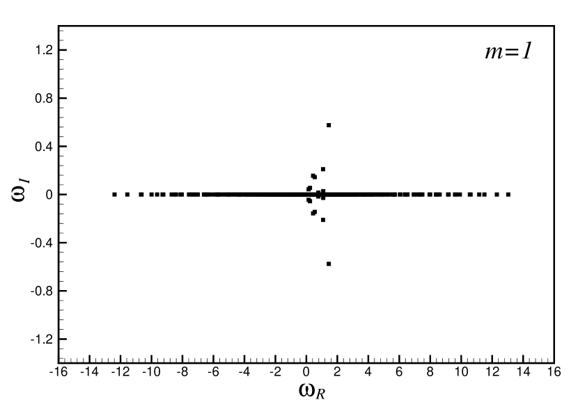
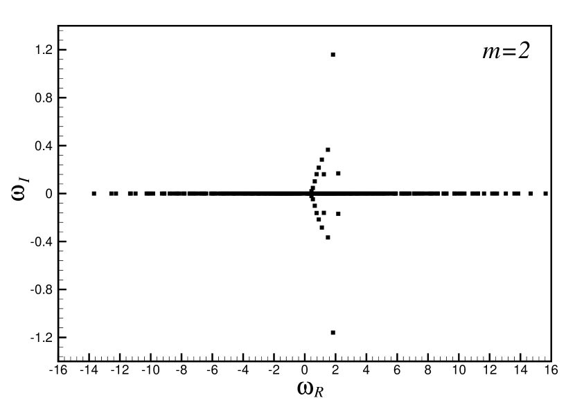
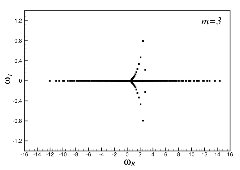
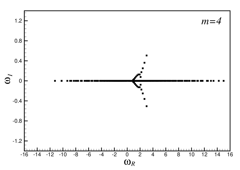
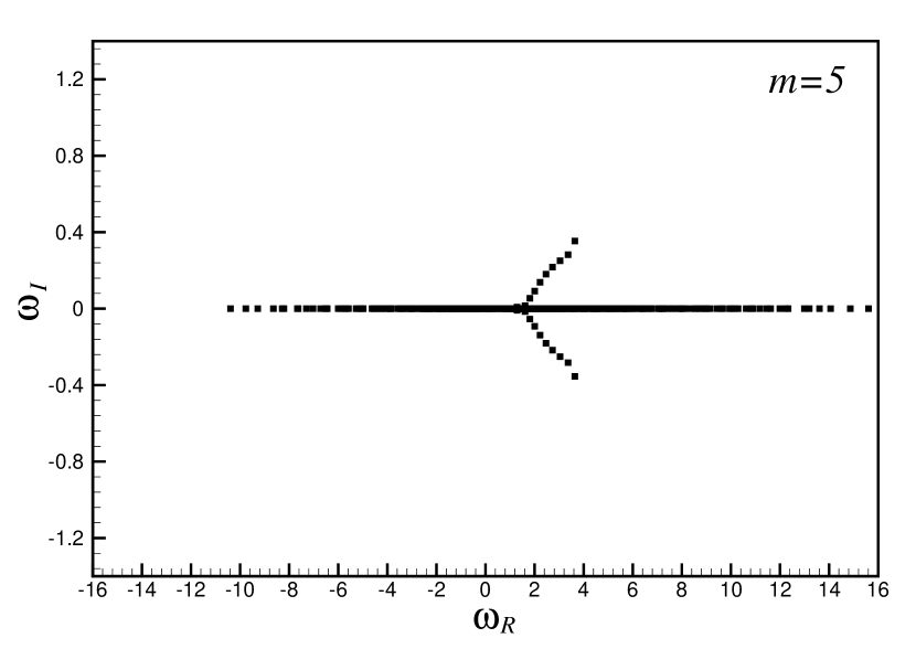
Figure 1.— Eigenfrequency spectra of a cored exponential disk with $v_{0}=1$, $R_{C}=1$ and $(N,\lambda,\alpha)=(6,1,0.42)$. Eigenfrequencies have been displayed for the azimuthal wavenumbers $0\leq m\leq 5$. The results correspond to $l_{\rm max}=10$ and $j_{\rm max}=15$ in the series expansion of the perturbed distribution function.

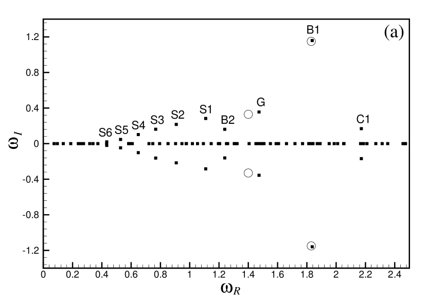
Figure 2.— (a) Zoomed eigenfrequency spectra (filled squares) of a cored exponential disk with $(N,\lambda,\alpha)=(6,1,0.42)$ for the azimuthal wavenumber $m=2$. The (isolated) bar mode has been labeled B1. The most prominent growing modes belong to a discrete family that bifurcates from a van Kampen mode. The members of this family, labeled as S1, S2, S3,$\cdots$, have spiral patterns. Circles show the eigenfrequencies of the fundamental and secondary modes calculated using Kalnajs’s (1977) method (see Table 4 in JH). (b) The eigenfrequency loci of the same model of panel a as $\alpha$ is increased continuously from $0.2$ to $0.42$. A few sample eigenfrequencies have been displayed on each locus.

Figure 3.— Mode shapes of the cored exponential disk for $R_{C}=1$, $v_{0}=1$ and $(N,\lambda,\alpha)=(6,1,0.42)$. Panels have been labeled by the corresponding mode name. The contour plots show the positive part of $\Sigma_{1}(R,\phi,0)$. The contour levels range from 10$\%$ to 90$\%$ of the maximum of $\Sigma_{1}(R,\phi,0)$ with increments of 10$\%$. The panel below each mode shape shows the amplitude of wave patterns as defined in equation (46).

4. MODES OF THE CORED EXPONENTIAL DISK

JH calculated barred and spiral modes of certain stellar disks for the wavenumber $m=2$. Among the models studied in JH, the cored exponential disk with the surface density profile

$$\Sigma_{D}(R)=\Sigma_{s}\exp\left(-\lambda\sqrt{1+R^{2}/R_{C}^{2}}\right),~{}~{}\lambda=\frac{R_{C}}{R_{D}},$$ (43)

and embedded in the field of the soft-centered logarithmic potential

$$V_{0}(R)=v_{0}^{2}\ln\sqrt{1+R^{2}/R_{C}^{2}},$$ (44)

is a viable model that resembles most features of realistic spirals. Here $R_{C}$ is the core radius, $R_{D}$ is the length scale of the exponential decay, and $\Sigma_{s}$ is a density scaling factor. The velocity of circular orbits in this model rises from zero at the galactic center and approaches to the constant value $v_{0}$ in outer regions where the light profile falls off exponentially. Jalali & Hunter (2005b) have derived the gravitational potential corresponding to $\Sigma_{D}(R)$. I denote this potential by $V_{D}(R)$. The gradient

$$F_{H}=\frac{d}{dR}\left[V_{0}(R)-V_{D}(R)\right],$$ (45)

will give the gravitational force of a spherical dark matter component, computed inside the galactic disk. The density profile of the dark component, $\rho_{H}$, can then be determined using $F_{H}$. The positiveness of $\rho_{H}$ imposes some restrictions on the physical values of $\lambda$ and $\alpha=G\Sigma_{s}R_{D}/v_{0}^{2}$ as Figure 5 in JH shows. For a given $\lambda$, $\alpha$ cannot exceed a critical value $\alpha_{cr}$. The parameter $\lambda$ determines the shape of the dark matter density profile. A model with $\lambda=1$ and $\alpha=\alpha_{cr}$ is maximal in the region where the rotation curve is rising. i.e., there is no dark matter in that region. Models with $\lambda>1$ and $\alpha=\alpha_{cr}$ are still maximal but only in the vicinity of the center for $R<R_{D}$. In such models the rotational velocity of stars due to dark matter ($v_{H}=\sqrt{RF_{H}}$) has a monotonically rising profile. For $\lambda<1$, dark matter penetrates into the galactic center and its density profile becomes cuspy in the limit of $\lambda\rightarrow 0$. The role of the parameter $\alpha$ is to control the fraction of dark to luminous matter. Models with $\alpha\ll\alpha_{cr}$ are dominated by dark matter.

JH introduced a family of equilibrium DFs that reproduces $\Sigma_{D}(R)$ and depends on an integer constant $N$. This parameter controls the population of near-circular orbits and the disk temperature: the parameter $Q$ of Toomre (1964) decreases by increasing $N$. The DFs of JH have an isotropic part that determines the fraction of radial orbits. That isotropic part, which reconstructs the central density of the equilibrium state, shrinks to central regions of the galaxy as $N$ increases.

I apply my new method to the cored exponential disks of JH and calculate the spectrum of $\omega=\omega_{R}+{\rm i}\omega_{I}$. Subsequently, the eigenvector $\textbf{{z}}_{0}$ is calculated from (37) and it is used in (19) to compute $a^{m}_{j}(t)=e^{-{\rm i}\omega t}a^{m}_{j}(0)$ and the perturbed density

$$\Sigma_{1}(R,\phi,t)=e^{\omega_{I}t}P_{m}(R)\cos\left[m\phi\!-\!\omega_{R}t\!+\!\vartheta_{m}(R)\right],$$ (46)

which is the real part of (10). $P_{m}(R)$ and $\vartheta_{m}(R)$ are the amplitude and phase functions of an $m$-fold circumferential wave that travels with the angular velocity $\omega_{R}/m$. The factor $e^{\omega_{I}t}$ shows the exponential growth/decay of the wave amplitude. I normalize all length, velocity, and time variables to $R_{C}$, $v_{0}$ and $R_{C}/v_{0}$, respectively, and set $G=R_{C}=v_{0}=1$.

I begin my case studies in §4.1 with a near maximal disk of $(N,\lambda,\alpha)$=$(6,1,0.42)$ and compute its eigenfrequency spectra for the wavenumbers $0\leq m\leq 5$. I then classify unstable $m=2$ modes of this model and investigate their evolution as the parameter $\alpha$ is varied. In §4.2 and §4.3, I study the behavior of unstable $m=2$ waves as the parameters $\lambda$ and $N$ are changed. The eigenfrequency spectrum of a model with an inner cutout is also computed and discussed in §4.4.

4.1. A Near Maximal Disk

I pick up the first model from Table 4 of JH with $(N,\lambda,\alpha)=(6,1,0.42)$ and start solving the eigensystem (37) with $(l_{\rm max},j_{\rm max})=(2,4)$ and increase these limits until complex eigenfrequencies converge. For an error threshold of $1\%$ the program terminates when $(l_{\rm max},j_{\rm max})=(10,15)$, which gives a size of $336\times 336$ for the matrix A. In such a circumstance, out of $336$ eigenfrequencies of A (for each wavenumber $m$), less than 15 pair have non-zero growth rates ($\omega_{I}\not=0$). Further increasing of $l_{\rm max}$ and $j_{\rm max}$ does not alter the number and location of complex eigenfrequencies in the $\omega$-plane. This shows that unstable modes do not constitute a continuous family.

Figure 1 displays the eigenfrequency spectra for the azimuthal wavenumbers $0\leq m\leq 5$. Eigenfrequencies on the real axis are oscillatory van Kampen modes. Their calculation requires evaluation of Cauchy’s principal value (Vandervoort, 2003) if one uses Kalnajs’s first order theory. In the present formalism, van Kampen modes are found together with growing modes without any special treatment. More van Kampen modes are obtainable by increasing the truncation limit $l_{\rm max}$ of Fourier terms in the $\theta_{R}$-direction. Toomre’s $Q$ is marginally greater than 1 for the model (Figure 7b in JH), and therefore, one could expect that the disk is stable for $m=0$ excitations (see top-left panel in Figure 1). The model is highly unstable for $m>0$ excitations although the average growth rate of unstable modes decreases for larger wavenumbers. It is evident that either unstable modes are isolated or they are grouped in discrete families. Depending on the wavenumber, there may be one or more discrete families. The most prominent family bifurcates from van Kampen modes. Members of this family have spiral patterns with multiple peaks in their $P_{m}(R)$ functions. The (global) fastest growing mode belongs to the spectrum of $m=2$. That is the bar mode of a two-member unstable family.

The length scale of Clutton-Brock functions has been set to $b=1.5$ for $m=2$ and $b=2$ for other wavenumbers. Changing this length scale slightly displaces the eigenfrequencies although the spectrum maintains its global pattern. Large values of $b$ lead to a better computation accuracy of extensive modes (with smaller pattern speeds), while compact bar modes show a rapid convergence for small values of $b$. Moreover, the suitable value of $b$ differs from one azimuthal wavenumber to another. Finding an optimum length scale that gives the best results for all modes and wavenumbers is an open problem yet to be investigated precisely. For the cored exponential disks with $0.5\leq R_{C},R_{D}\leq 2$, working in the range $1\leq b\leq 2.5$ gives reasonable results.

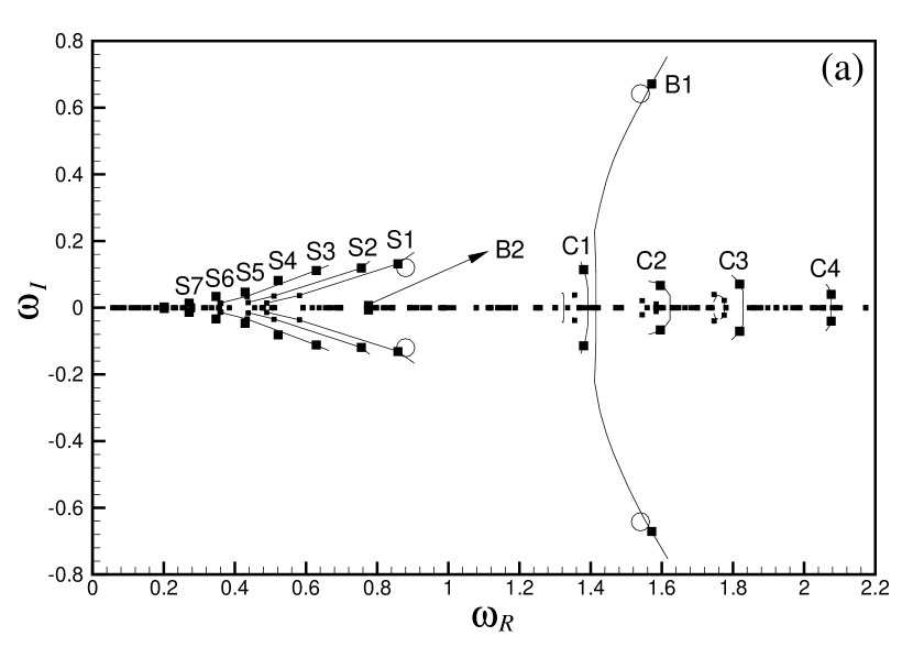
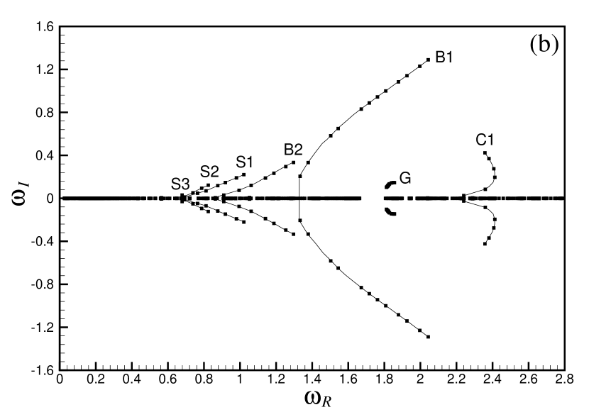
Figure 4.— (a) Eigenfrequency loci (solid lines) of cored exponential disks with $(N,\lambda)=(6,0.625)$ for $0.2\leq\alpha\leq 0.36$. Large squares show the eigenfrequency spectrum of a model with $\alpha=0.34$, and circles show the eigenfrequencies of the fundamental and secondary modes calculated using Kalnajs’s method (see Table 4 in JH) for $\alpha=0.34$. (b) Same as panel a but for models with $(N,\lambda)=(6,2)$ and $0.25\leq\alpha\leq 0.6$. Some sample eigenfrequencies have been demonstrated on each locus.

For $m=2$, I have zoomed out and plotted in Figure 2a the portion of the spectrum that contains growing modes. The first and second modes reported in Table 4 of JH have been shown by circles in the same figure. The most unstable mode (labeled as B1) is a compact, rapidly rotating bar. The majority of unstable modes belong to a discrete spiral family that bifurcates from a van Kampen mode with $\omega\approx 0.43$. I have labeled these modes by S1,$\cdots$,S6. The number of density peaks along the spiral arms is proportional to the integer number in the mode name. Both B2 and G are double peaked spirals but I have classified B2 as a bar mode, and collected it with B1 in a two member family, for it takes a bar-like structure when it is stabilized by decreasing $\alpha$. I classify mode G as an isolated mode because it does not behave similar to either of S- or B-modes as the model parameters vary. There is another isolated mode in the spectrum, C1, which exhibits a spiral pattern. By decreasing $\lambda$, mode C1 joins a new family of spiral modes, which are accumulated near the galactic center (see §4.2).

Reducing $\alpha$ increases the abundance of dark matter and according to Toomre (1981) and JH the growth rate of modes should decrease. My calculations show that by reducing $\alpha$, spiral modes are affected sooner and more effective than the bar mode, and they join to the stationary modes, one by one from the location of the bifurcation point until the whole S-family disappears. This is a generic scenario for all $\lambda\geq 1$ models regardless of the disk temperature controlled by $N$. Solid lines in Figure 2b show the eigenfrequency loci of a model with $(N,\lambda)=(6,1)$ as $\alpha$ increases from $0.2$ to $0.42$. It is evident that mode B1 is destabilized through a pitchfork bifurcation while the loci of modes B2 and C1, and S-modes exhibit a tangent bifurcation. All modes except mode G are stable for $\alpha<0.23$. Surprisingly, mode G resists against stabilization even for very small values of $\alpha$. This indicates that mode G is not characterized by the fraction of dark to luminous matter. In §4.2 and §4.3, I will show that this mode is highly sensitive to the variations of $\lambda$ and $N$. According to my computations (e.g., Figure 2b), by increasing $\alpha$ all S-modes are born at the same bifurcation frequency $\omega_{S}\approx 0.43$, but mode B2 comes out from a van Kampen mode with $\omega_{B}\approx 0.83$. This result completely rules out any skepticism that mode B2 is a member of S-family.

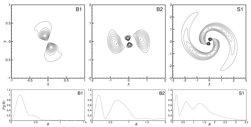
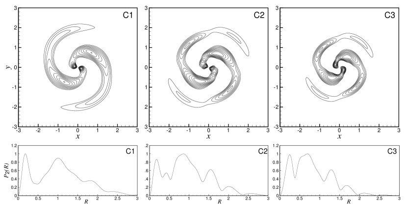
Figure 5.— Same as Figure 3 but for a model with $(\lambda,\alpha)=(0.625,0.34)$. The fastest growing spiral mode, S1, has also been found by JH. Modes C1, C2 and C3 have emerged due to dark matter presence at the galactic center. They shrink to central regions and grow slower as their pattern speed increases.

Figure 3 displays the wave patterns and amplitude functions of modes B1, B2, G, S1, S2 and S3. It is seen that the patterns of S-modes rotate slower and become more extensive as the mode number increases. Mode S6, which is at the bifurcation point of the spiral family, has the largest extent. Eight wave packets of this mode are distributed by a phase shift of 90 degrees along major spiral arms. Mode G has at most two density peaks on its major spiral arms but the magnitude of its second peak increases as the disk is cooled. Modes B1, B2, S1, S2 and S3 are, respectively, analogous to modes A, B, C, E and F of a Gaussian disk explored in Toomre (1981). There are three low-speed modes in Figure 11 of Toomre (1981) that have not been labeled, but they are analogs of modes S4, S5 and S6. Mode G and Toomre’s mode D also have some similarities but are of different origins (see §5). None of them can be stabilized only by increasing the fraction of dark matter.

Figure 2a shows that the fundamental mode obtained by JH coincides with mode B1. The wave pattern of mode B1 (displayed in Figure 3) is identical to the mode shape computed using Kalnajs’s theory and demonstrated in Figure 8 of JH. JH found a secondary mode which lies between modes B2 and G. That mode is also a double-peaked spiral and it is not easy to identify its true nature unless we investigate its evolution as the model parameters vary. By comparing Figure 10a of JH with Figure 2b, one can see that both mode B2 and the secondary mode of JH are destabilized through a tangent bifurcation while mode G has a different nature. The bifurcation frequency of mode B2 that I find ($\omega_{B}\approx 0.83$) matches very well with the frequency of the stabilized secondary mode of JH (see Figure 10a in JH but note that their vertical axis indicates $\Omega_{p}=\omega_{R}/2$). Therefore, I conclude that the secondary mode of JH is indeed mode B2 although it seems to be closer to mode G. The existing discrepancy is due to different length scale of Clutton-Brock functions that JH have used for finding the secondary mode. By adjusting $b$ one can improve the location of B2. However, this is an unnecessary attempt given the fact that mode B2 has already been identified, and the computation accuracy of other eigenfrequencies has an impressive level.

4.2. Variations of $\lambda$

The parameter $\lambda$ controls the density profile of the dark matter component, specifically near the galactic center. The fraction of dark to luminous matter has its minimum value in marginal models with $\alpha\approx\alpha_{cr}$. I choose a marginal $\lambda<1$ model with $(N,\lambda,\alpha)=(6,0.625,0.34)$, which has also been investigated by JH. Figure 4a shows the portion of the spectrum that contains complex eigenfrequencies of this model. The spectrum has been computed for $b=1.5$. Although $m=2$ bar and spiral modes survive in this model, their pattern speeds and growth rates drop considerably. Mode G has been wiped out of existence by dark matter penetration into the center, and four unstable modes (C1, C2, C3 and C4) have emerged that constitute a new family of spiral modes. They populate the central regions of the disk in most of $\lambda<1$ models. Again, the location of eigenfrequencies obtained by JH have been marked by circles. The agreement between the results of JH and the present study is very good and the variance is less than $2\%$.

The population of spiral modes is changed by varying $\alpha$, and the eigenfrequencies of unstable modes are altered significantly. Solid lines in Figure 4a show the loci of growing modes as $\alpha$ increases from $0.2$ to $\alpha_{cr}\approx 0.36$. Similar to the previous $\lambda=1$ model, S-modes and mode B1 are destabilized through tangent and pitchfork bifurcations, respectively. All C-modes are born by a pitchfork bifurcation although some minor modes of the same nature come and go as $\alpha$ varies. The loci of modes B1 and S1 (in Figure 4a) are in harmony with the results of Kalnajs’s method plotted in Figure 10b of JH. It is noted that the locus of mode B1 steeply joins the real axis, well before stabilizing the S-modes. This is how slowly growing spirals may dominate a stellar disk.

There are no new families of growing modes in $\lambda>1$ models. Dark matter in these models induces a rising rotation curve on the disk stars (see Figure 6 in JH) and the population of S-modes declines. The growth rate of mode B2 increases proportional to $\lambda$, but that of mode G falls off although mode G is still robust against the variations of $\alpha$. Mode G has its maximum growth rate in $\lambda=1$ models, which suggests that it must be a self-gravitating response of the luminous matter that involves only the potential of the disk, $V_{D}$. The function $P_{2}(R)$ of mode C1 loses its minor peaks and becomes smoother as $\lambda$ increases. Figure 4b shows the eigenfrequency loci of models with $(N,\lambda)=(6,2)$ as $\alpha$ increases from $0.25$ to $\alpha_{cr}\approx 0.6$. The eigenfrequency loci of modes C1 and B2, and S-modes (as $\alpha$ varies) are similar to $\lambda=1$ models, but the locus of mode B1 loses its steepness and stretches towards small pattern speeds in an approximately linear form until it joins the real $\omega_{R}$-axis. The bifurcation frequency of mode B2 differs from S-modes and it is larger.

Figure 5 shows the wave patterns of modes B1, B2, S1, C1, C2 and C3 for the model with $(N,\lambda,\alpha)=(6,0.625,0.34)$. The (isolated) mode B1 is still a single-peaked bar although its edge is more extensive as the flat part of its $P_{2}(R)$ plot indicates. Mode S1 is a triple-peaked spiral (as before) and mode B2 is being stabilized ($\omega_{\rm B2}=0.775+0.007{\rm i}$). It is seen that mode B2 has a bar-like structure, which justifies its classification as the secondary bar mode. The pattern of S1 and its $P_{2}(R)$ plot can be compared with Figure 9 in JH. The agreement is quite satisfactory. There is a remarkable difference between the patterns of C- and S-modes although both families have spiral structures. In contrast to S-modes that become more extensive as their growth rate decays, C-modes are shrunk to central regions because their pattern speed increases. C-modes are also a bifurcating family, but their bifurcation point lies on large pattern speeds associated with the azimuthal frequency ($\Omega_{\phi}$) of central stars.

The parameters $\alpha$ and $\lambda$ are essentially controlling the fraction and density profile of dark matter component, respectively. However, the radial velocity dispersion $\sigma_{R}$ of the equilibrium state is also playing an important role in the perturbed dynamics. $\sigma_{R}$ is an indicator of the initial temperature of the disk. Evans & Read (1998b) had already pointed out that the pitch angle of spiral patterns decreases when $\sigma_{R}\rightarrow 0$ (see their Figure 7). Apart from this morphological implication, can the variation in the disk temperature affect the modal content? In the following subsection, I trace the evolution of growing waves by changing the disk temperature and show that the population of S-modes is larger in rotationally supported, cold disks.

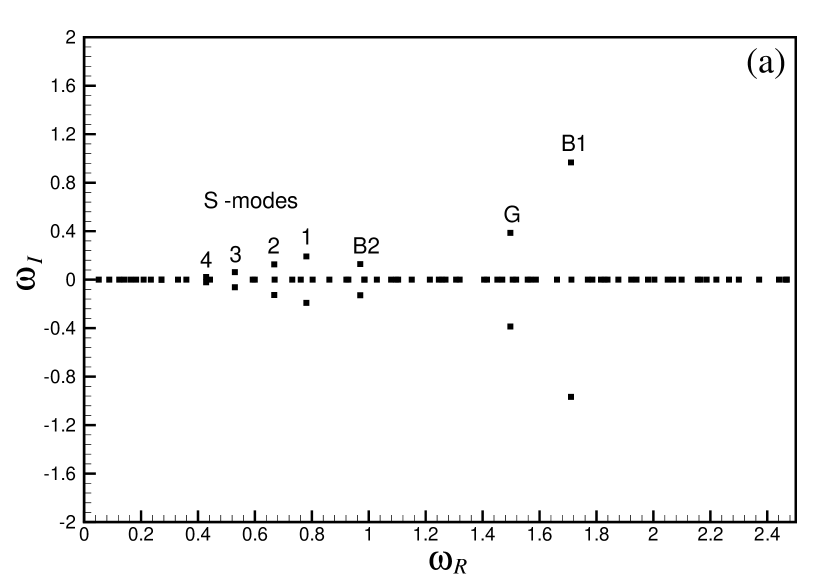
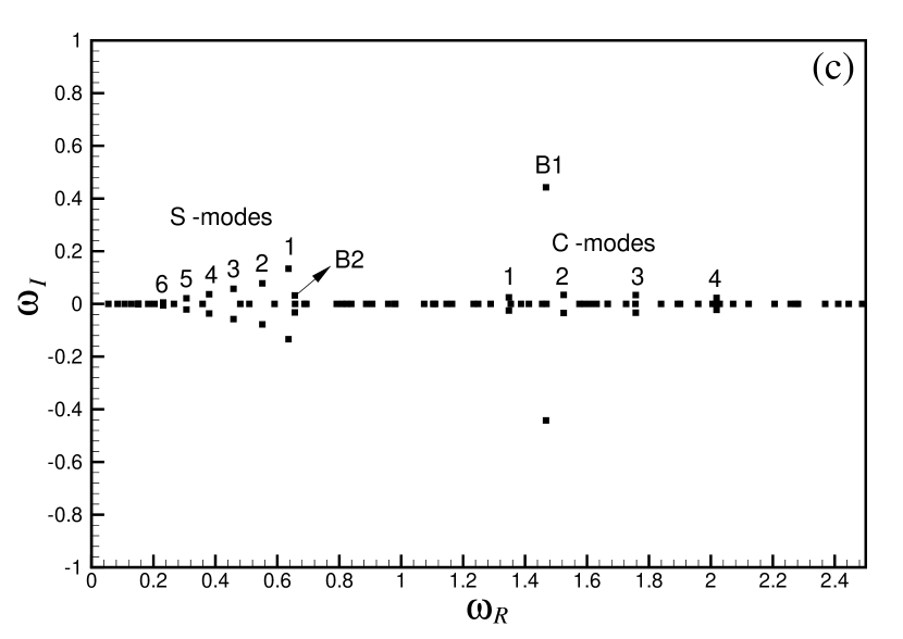
Figure 6.— The evolution of the eigenfrequency spectra as the disk temperature drops from left ($N=4$) to right ($N=8$) panels. Top and bottom panels correspond to $(\lambda,\alpha)=(1,0.42)$ and $(\lambda,\alpha)=(0.625,0.34)$, respectively.

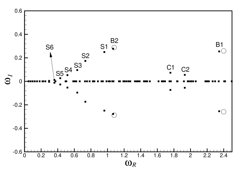
Figure 7.— Eigenfrequency spectrum of a cutout model with $L_{0}=0.1$ and $(N,\lambda,\alpha)=(6,1,0.42)$. Circles show the eigenfrequencies found by JH using Kalnajs’s theory.

4.3. Variations of the Disk Temperature

The parameter $N$ of the DFs of JH controls the disk temperature by adjusting the size of the isotropic core and the population of near circular orbits. As $N$ increases, the streaming velocity $\langle v_{\phi}\rangle$ approaches the rotational velocity of circular orbits and the stellar disk is cooled. Figure 6 displays the eigenfrequencies of previous $(\lambda,\alpha)=(1,0.42)$ and $(\lambda,\alpha)=(0.625,0.34)$ models for $N=4$ and $N=8$. The spectra for the intermediate value of $N=6$ have already been shown in Figures 2a and 4a.

Increasing $N$ gives birth to more S-modes while the bifurcation point of the family is preserved. As a new member is born at the bifurcation point, other members including mode S1, are pushed away from the real axis on a curved path. This behavior is observed in both models but the branch of S-family in the model with $(\lambda,\alpha)=(0.625,0.34)$ stays closer to the real axis than the other model. The growth rates of C-modes increase remarkably as the disk is cooled. Despite mode B1 which rotates and grows faster in cold disks, mode B2 grows faster in warmer disks. Variation in the disk temperature changes the eigenfrequency of mode G more effective than what $\alpha$ could, but nothing is more influential than the role of $\lambda$.

Another consequence of cooling the stellar disk is that $m=0$ waves are no longer stable. The parameter $Q$ of Toomre was marginally greater than unity for $N=6$ models. For $N=8$, I find $Q<1$ over an annular region because the plot of $Q$ versus $R$ exhibits a minimum at some finite radius (e.g., Figure 7 of JH). For instance, I find three growing $m=0$ modes for the model $(N,\lambda,\alpha)=(8,1,0.42)$. They correspond to pure complex eigenfrequencies $\omega_{1}=0.621{\rm i}$, $\omega_{2}=0.494{\rm i}$ and $\omega_{3}=0.238{\rm i}$. Mode shapes have (obviously) ringed structures but the number of rings, which is identical to the number of peaks of $P_{0}(R)$, depends on the growth rate. The modes associated with $\omega_{1}$, $\omega_{2}$ and $\omega_{3}$ have three, four and five rings, respectively. Ring modes are very sensitive to the variations of model parameters and they are suppressed by decreasing $\lambda$ and $\alpha$.

4.4. The Effect of an Inner Cutout

In order to simulate an immobile bulge, which does not respond to density perturbations, JH utilized an inner cutout function of the form

$$H_{\rm cut}=1-e^{-\left(J_{\phi}/L_{0}\right)^{2}},$$ (47)

where $L_{0}$ is an angular momentum scale. Multiplying $H_{\rm cut}$ by the self-consistent DF of the equilibrium state, prohibits the stars with $J_{\phi}<L_{0}$ from participating in the perturbed dynamics. Consequently, incoming waves are reflected at some finite radius and the innermost wave packets of multiple-peaked modes are diminished. My calculations show that all S-modes survive in cutout models, mode G disappears, and the growth rate of mode B2 increases. The pattern speed of mode B1 is boosted so that the corotation resonance is destroyed, but its growth rate drops drastically. Figure 7 shows the eigenfrequency spectrum of a model with $L_{0}=0.1$ and $(N,\lambda,\alpha)=(6,1,0.42)$. Circles show the eigenfrequencies found by JH. Again, the agreement between the results of JH and the present work is very good. The reason that I have identified mode B2 as the second member of B-family, and not the most unstable S-mode, is that its $P_{2}(R)$ function has an evolved double-peaked structure (see Figure 11 in JH) and its locus versus $\alpha$ does not emerge from the same bifurcation frequency of S-modes. Disappearance of mode G in cutout models confirms my earlier note that it is a self-gravitating mode.

5. DISCUSSIONS

There are similarities between mode G of this study and Toomre’s (1981) mode D. Both of these modes resist against stabilization by increasing the fraction of dark to luminous matter and they have at most double peaks on their spiral arms. Nonetheless, these modes are not the same because mode G is amplified through a feedback from the galactic center but Toomre’s mode D has been identified as an edge mode. A question remains to be answered: why Toomre (1981) did not detect mode G and I do not find an edge mode? The most convincing explanation is that to excite a self-gravitating wave inside the core of the stellar component, the governing potential in that region should mainly come from the self-gravity of stars. This requirement is fulfilled in my $\lambda\geq 1$ models for $R<R_{D}$. However, the completely flat rotation curve imposed by Toomre (1981) nowhere follows the rotational velocity induced by the self-gravity of stars and it prohibits the Gaussian disk from developing a G-like mode. On the other hand, I don’t find an edge mode because the density profile of the cored exponential disk does not decay as steep as the Gaussian disk to create an outer boundary at some finite radius for reflecting the outgoing waves.

Similar to the first order analysis of §3, Polyachenko’s (2005) approach results in the full spectrum of eigenfrequencies for a given azimuthal wavenumber. There are some differences between his method and the present formulation. Polyachenko directly uses Poisson’s integral to establish a point-wise relation in the action space between the Fourier components of the perturbed DF and its self-consistent potential. Combination of equations (5) and (9) in his paper is analogous to equation (21) in this paper. The main departure of the two theories is in the way that the linearized CBE is treated. Polyachenko forces a point-wise fulfillment of the CBE in the action space while the present method works with a weighted residual form of the CBE.

A point-wise formulation poses a challenge for the numerical calculation of the eigenvalues and their conjugate eigenvectors. According to the bar charts of JH, at least ten Fourier components ($-3\leq l\leq 6$) are needed in the $\theta_{R}$-direction to assure a credible convergence of $f_{1}$ in a typical soft-centered galaxy model. Therefore, if one chooses a grid of $n_{a}\times n_{a}$ in the action space, Polyachenko’s eigenvector F will have a dimension of $10\times n_{a}\times n_{a}$. Therefore, for a very coarse grid with $n_{a}=21$ that Polyachenko uses, the unknown eigenvector will have a dimension of 4410. This number must be compared with the dimension of $\textbf{{z}}_{0}$ in equation (37). That is indeed $n_{\rm max}=336$ for the most accurate calculations carried out by setting $(l_{\rm max},j_{\rm max})=(10,15)$ which means that $21$ Fourier components in the $\theta_{R}$-direction and $16$ expansion terms in the $R$-direction have been taken into account. Noting that the definite integrals ${\cal I}^{ml}_{jk}$ and $\Lambda^{ml}_{jk}$ are independently evaluated over the action space with any desired accuracy, the present theory proves to be more efficient for eigenmode calculation (in the linear regime) than other existing alternatives.

The agreement between the results of this work and those of JH, who have used Kalnajs’s method, is impressive. There is only a discrepancy in the results for a double-peaked spiral mode of $\lambda=1$ models. In fact, these models have two double-peaked modes, modes B2 and G, and JH find mode B2. The origin of discrepancies was attributed to the length scale of Clutton-Brock functions, $b$, which is a fixed number for the whole spectrum of a given azimuthal wavenumber. Provided that JH optimized $b$ for each growing mode that they calculated (see also §4.1), some minor deviations from the results of this paper are reasonable. In most cases the algorithm used by JH converges to mode B1 and the fastest rotating S-mode. They capture mode B2 only if its growth rate is large enough. Other modes remain unexplored because Newton’s method needs an initial guess of $\omega$, which has a little chance to be in the basin of attraction of the other members of S-family. The separation of eigenfrequencies near the bifurcation point of S-modes is very small and one could anticipate complex boundaries for the basins of attraction of these eigenfrequencies. Thus, there is no guarantee that successive Newton’s iterations keep an estimated eigenfrequency on the same basin that it was initially. Nevertheless, in Kalnajs’s formulation, a systematic search for all growing modes is possible by introducing the mathematical eigenvalue (Zang, 1976; Evans & Read, 1998b) and investigating its loci as the pattern speed and growth rate vary.

6. CONCLUSIONS

After three decades of Kalnajs’s (1977) publication, it was not known exactly whether growing modes of stellar systems appear as distinct roots in the eigenfrequency space or they belong to continuous families as van Kampen modes do. In this paper, I attempted to answer this question using the Galerkin projection of the CBE and unveiled the full eigenfrequency spectrum of a stellar disk. I showed that similar to gaseous disks (Asghari & Jalali, 2006), majority of growing modes emerge as discrete families through a bifurcation from stationary modes. There are some exceptions for this rule, the most important of which are the isolated bar and G modes.

The model that I used to test my method allows for dark matter presence as a spherical component, whose potential inside the galactic disk contributes to the rotational velocity of stars. By varying the parameters of the model, and investigating the eigenfrequencies and their associated mode shapes, I showed that it is not the fraction of dark to luminous matter that controls the variety of growing modes. What determines that variety is indeed the shape of the dark matter density profile controlled by the parameter $\lambda=R_{C}/R_{D}$. My survey in the parameter space revealed that the concentration of dark matter in the galactic center ($\lambda<1$) destroys mode G and weakens the growth of B-modes substantially. Emergence of spiral C-modes that accumulate near the galactic center is another remarkable consequence of dark matter presence in central regions of a cored stellar disk.

Although the solution of the Galerkin system showed a credible convergence of the series expansions, the existence of strong solutions for the CBE, in its full nonlinear form, is still an open problem. It has been known for years that van Kampen modes make a complete set (Case, 1959), and therefore, they may be used for a series representation of stationary oscillations. But there is not a mathematical proof for the completeness of the discrete families of growing modes. In other words, whether an observed galaxy can be assembled using the modes of a linear eigensystem, requires further analysis.

In the second part of this study, I will investigate the mechanisms of wave interactions in the nonlinear regime and will probe the mass and angular momentum transfer between waves of different Fourier numbers.

Appendix A WEIGHTED RESIDUAL FORM OF THE COLLISIONLESS BOLTZMANN EQUATION

Let me define a nonlinear operator ${\cal A}$ and denote $\textbf{{u}}^{(\ell)}$ as the $\ell$th prolongation (Olver, 1993) of the physical quantity $u$ in the domain of independent variables. Assume a (nonlinear) partial differential equation

$${\cal A}\left(u^{(\ell)},x,t\right)=0,$$ (A1)

and its associated initial and boundary conditions that govern the evolution of $u(x,t)$ in the domain of the spatial variable $x$ and the time $t$. A weighted residual method (Finlayson, 1972) attempts to find an approximate solution of the form

$$u(x,t)=\sum_{k=1}^{k_{\rm max}}a_{k}(t)\varphi_{k}(x),$$ (A2)

through determining the time-dependent functions $a_{k}(t)$ for a given set of trial (basis) functions $\varphi_{k}(x)$. The trial functions should satisfy the boundary conditions and be linearly independent. Using (A2) and taking the inner product of (A1) by some weighting functions $W_{k^{\prime}}(x)$, yield the determining equations of $a_{k}(t)$ as

$$\left({\cal A},W_{k^{\prime}}\right)\equiv\int{\cal A}W_{k^{\prime}}dx=0,~{}~{}k^{\prime}=1,2,\cdots,k_{\rm max}.$$ (A3)

There are several procedures for choosing $W_{k^{\prime}}(x)$ and each procedure has its own name. The method with $W_{k^{\prime}}=\varphi_{k^{\prime}}$ is called the Bubnov-Galerkin, or simply the Galerkin method. The Petrov-Galerkin method is associated with $W_{k^{\prime}}\not=\varphi_{k^{\prime}}$. The well-known collocation method uses Dirac’s delta functions for the weighting purpose. There is an alternative interpretation for the inner product $\left({\cal A},W_{k^{\prime}}\right)=0$. That is projecting the equation ${\cal A}=0$ on a subspace spanned by the weighting function $W_{k^{\prime}}$. Therefore, equation (A3) is often called the Galerkin projection of (A1). In what follows, I use the Petrov-Galerkin method and construct the weighted residual form of the CBE.

Assume the functions $U(\Theta,\textbf{{J}})$ and $V(\Theta,\textbf{{J}})$, and define their inner product over the action-angle space as

$$\left(U,V\right)=\int\int U(\Theta,\textbf{{J}})V(\Theta,\textbf{{J}})d\textbf{{J}}d\Theta.$$ (A4)

Taking the inner product of the perturbed CBE by the weighting functions $W^{ml}_{j}(\Theta,\textbf{{J}})=\Psi^{ml}_{j}(\textbf{{J}})e^{-{\rm i}\left(l\theta_{R}+m\theta_{\phi}\right)}$ gives

$$\left(\frac{\partial f_{1}}{\partial t},W^{ml}_{j}\right)=-\left(\left[f_{1},{\cal H}_{0}\right],W^{ml}_{j}\right)-\left(\left[f_{0},{\cal H}_{1}\right],W^{ml}_{j}\right)-\left(\left[f_{1},{\cal H}_{1}\right],W^{ml}_{j}\right).$$ (A5)

Note that the CBE is the governing equation of the perturbed DF whose trial functions are $\Phi^{ml}_{j}(\textbf{{J}})$. With my choice of the weighting function (as above) I am following the Petrov-Galerkin method. On substituting (8) and (21) in (A5) and after some rearrangements of summations, one obtains

$${\rm i}\sum_{m^{\prime},l^{\prime}}\sum_{j^{\prime}}\delta_{m,m^{\prime}}\delta_{l,l^{\prime}}{{\rm d}\over dt}d^{m^{\prime}l^{\prime}}_{j^{\prime}}(t)\int d\textbf{{J}}\Psi^{ml}_{j}(\textbf{{J}})\Phi^{m^{\prime}l^{\prime}}_{j^{\prime}}(\textbf{{J}})=$$ (A6)

$$\sum_{m^{\prime},l^{\prime}}\sum_{j^{\prime}}\delta_{m,m^{\prime}}\delta_{l,l^{\prime}}d^{m^{\prime}l^{\prime}}_{j^{\prime}}(t)\int d\textbf{{J}}\left(l^{\prime}\Omega_{R}+m^{\prime}\Omega_{\phi}\right)\Psi^{ml}_{j}(\textbf{{J}})\Phi^{m^{\prime}l^{\prime}}_{j^{\prime}}(\textbf{{J}})$$

$$- \sum_{m^{\prime},l^{\prime}}\sum_{j^{\prime}}\delta_{m,m^{\prime}}d^{m^{\prime}l^{\prime}}_{j^{\prime}}(t)\sum_{k}\left[{4\pi^{2}\over D_{k}(m^{\prime})}\right]\Lambda^{m^{\prime}l^{\prime}}_{kj^{\prime}}\int d\textbf{{J}}\left(l{\partial f_{0}\over\partial J_{R}}+m^{\prime}{\partial f_{0}\over\partial J_{\phi}}\right)\Psi^{m^{\prime}l}_{j}(\textbf{{J}})\Psi^{m^{\prime}l}_{k}(\textbf{{J}})$$

$$+ \sum_{m^{\prime},l^{\prime}}\sum_{j^{\prime}}\sum_{m^{\prime\prime},l^{\prime\prime}}\sum_{j^{\prime\prime}}\delta_{m^{\prime\prime},(m-m^{\prime})}d^{m^{\prime}l^{\prime}}_{j^{\prime}}(t)d^{m^{\prime\prime}l^{\prime\prime}}_{j^{\prime\prime}}(t)\sum_{k}\left[{4\pi^{2}\over D_{k}(m^{\prime\prime})}\right]\Lambda^{m^{\prime\prime}l^{\prime\prime}}_{kj^{\prime\prime}}$$

$$\times \Biggl{[}\int d\textbf{{J}}\Psi^{ml}_{j}(\textbf{{J}})\Phi^{m^{\prime}l^{\prime}}_{j^{\prime}}(\textbf{{J}})\left(l^{\prime}{\partial\over\partial J_{R}}+m^{\prime}{\partial\over\partial J_{\phi}}\right)\Psi^{m^{\prime\prime}(l-l^{\prime})}_{k}(\textbf{{J}})$$

$$\qquad-\int d\textbf{{J}}\Psi^{ml}_{j}(\textbf{{J}})\Psi^{m^{\prime\prime}(l-l^{\prime})}_{k}(\textbf{{J}})\left((l-l^{\prime}){\partial\over\partial J_{R}}+m^{\prime\prime}{\partial\over\partial J_{\phi}}\right)\Phi^{m^{\prime}l^{\prime}}_{j^{\prime}}(\textbf{{J}})\Biggr{]},$$

where $-m_{\rm max}\leq m,m^{\prime},m^{\prime\prime}<m_{\rm max}$, $-l_{\rm max}\leq l,l^{\prime},l^{\prime\prime}\leq l_{\rm max}$ and $0\leq j,j^{\prime},j^{\prime\prime},k\leq j_{\rm max}$. Using equation (22) and carrying out the index mappings $(m,l,j)\rightarrow p$, $(m^{\prime},l^{\prime},j^{\prime})\rightarrow q$ and $(m^{\prime\prime},l^{\prime\prime},j^{\prime\prime})\rightarrow r$ one may introduce the arrays

$$M_{pq} = \delta_{m,m^{\prime}}\delta_{l,l^{\prime}}\int d\textbf{{J}}\Psi^{ml}_{j}(\textbf{{J}})\Phi^{m^{\prime}l^{\prime}}_{j^{\prime}}(\textbf{{J}}),$$ (A7)

$$C_{pq} = \delta_{m,m^{\prime}}\Biggl{[}\delta_{l,l^{\prime}}\int d\textbf{{J}}\left(l^{\prime}\Omega_{R}+m^{\prime}\Omega_{\phi}\right)\Psi^{ml}_{j}(\textbf{{J}})\Phi^{m^{\prime}l^{\prime}}_{j^{\prime}}(\textbf{{J}})$$ (A8)

$$\qquad\qquad-\sum_{k=0}^{j_{\rm max}}\left[{4\pi^{2}\over D_{k}(m^{\prime})}\right]\Lambda^{m^{\prime}l^{\prime}}_{kj^{\prime}}\int d\textbf{{J}}\left(l{\partial f_{0}\over\partial J_{R}}+m^{\prime}{\partial f_{0}\over\partial J_{\phi}}\right)\Psi^{m^{\prime}l}_{j}(\textbf{{J}})\Psi^{m^{\prime}l}_{k}(\textbf{{J}})\Biggr{]},$$

$$K_{pqr} = \delta_{m^{\prime},(m-m^{\prime\prime})}\delta_{l^{\prime},(l-l^{\prime\prime})}\sum_{k=0}^{j_{\rm max}}\left[{4\pi^{2}\over D_{k}(m^{\prime\prime})}\right]\Lambda^{m^{\prime\prime}l^{\prime\prime}}_{kj^{\prime\prime}}$$ (A9)

$$\times\Biggl{[}\int d\textbf{{J}}\Psi^{ml}_{j}(\textbf{{J}})\Phi^{m^{\prime}l^{\prime}}_{j^{\prime}}(\textbf{{J}})\left(l^{\prime}{\partial\over\partial J_{R}}+m^{\prime}{\partial\over\partial J_{\phi}}\right)\Psi^{m^{\prime\prime}l^{\prime\prime}}_{k}(\textbf{{J}})$$

$$\qquad-\int d\textbf{{J}}\Psi^{ml}_{j}(\textbf{{J}})\Psi^{m^{\prime\prime}l^{\prime\prime}}_{k}(\textbf{{J}})\left(l^{\prime\prime}{\partial\over\partial J_{R}}+m^{\prime\prime}{\partial\over\partial J_{\phi}}\right)\Phi^{m^{\prime}l^{\prime}}_{j^{\prime}}(\textbf{{J}})\Biggr{]}.$$

Consequently, equation (A6) takes the following matrix form

$${\rm i}\sum_{q=1}^{n_{\rm max}}M_{pq}{d\over dt}z_{q}(t)=\sum_{q=1}^{n_{\rm max}}C_{pq}z_{q}(t)+\sum_{q,r=1}^{n_{\rm max}}K_{pqr}z_{q}(t)z_{r}(t),~{}~{}z_{p}(t)\equiv d^{ml}_{j}(t),~{}~{}p=1,2,\cdots,n_{\rm max}.$$ (A10)

Let the matrix $\textbf{{M}}^{-1}=[M^{-1}_{pq}]$ be the inverse of $\textbf{{M}}=[M_{pq}]$ and left-multiply (A10) by $\textbf{{M}}^{-1}$ to get

$${\rm i}{d\over dt}z_{p}(t)=\sum_{q=1}^{n_{\rm max}}A_{pq}z_{q}(t)+\sum_{q,r=1}^{n_{\rm max}}B_{pqr}z_{q}(t)z_{r}(t),~{}~{}\textbf{{A}}=\textbf{{M}}^{-1}\cdot\textbf{{C}},~{}~{}B_{pqr}=\sum_{s=1}^{n_{\rm max}}M^{-1}_{ps}K_{sqr}.$$ (A11)

Evaluation of the integrands in (A9) will be considerably simplified if one avoids the partial derivatives of $\Phi^{ml}_{j}(\textbf{{J}})$ through integrating (A9) by parts. That gives

$$K_{pqr}= \delta_{m^{\prime},(m-m^{\prime\prime})}\delta_{l^{\prime},(l-l^{\prime\prime})}\sum_{k=0}^{j_{\rm max}}\left[{4\pi^{2}\over D_{k}(m^{\prime\prime})}\right]\Lambda^{m^{\prime\prime}l^{\prime\prime}}_{kj^{\prime\prime}}$$

$$\times\biggl{\{} \int{\rm d}\textbf{{J}}\Psi^{ml}_{j}(\textbf{{J}})\Phi^{m^{\prime}l^{\prime}}_{j^{\prime}}(\textbf{{J}})\left(l{\partial\over\partial J_{R}}+m{\partial\over\partial J_{\phi}}\right)\Psi^{m^{\prime\prime}l^{\prime\prime}}_{k}(\textbf{{J}})$$ (A12)

$$+ \int d\textbf{{J}}\Phi^{m^{\prime}l^{\prime}}_{j^{\prime}}(\textbf{{J}})\Psi^{m^{\prime\prime}l^{\prime\prime}}_{k}(\textbf{{J}})\left(l^{\prime\prime}{\partial\over\partial J_{R}}+m^{\prime\prime}{\partial\over\partial J_{\phi}}\right)\Psi^{ml}_{j}(\textbf{{J}})\biggr{\}}.$$

When all stars move on prograde orbits, the equilibrium DF takes the form $f_{0}(\textbf{{J}})=H(J_{\phi})f^{P}_{0}(\textbf{{J}})$ where $H$ is the Heaviside function. Upon using (33), this contributes a term including Dirac’s delta function $\delta(J_{\phi})$ to the trial functions. Thus, the following boundary terms

$$K^{b}_{pqr}\! = \!\delta_{m^{\prime},(m-m^{\prime\prime})}\delta_{l^{\prime},(l-l^{\prime\prime})}\sum_{k=0}^{j_{\rm max}}\left[{4\pi^{2}\over D_{k}(m^{\prime\prime})}\right]\Lambda^{m^{\prime\prime}l^{\prime\prime}}_{kj^{\prime\prime}}$$

$$\times\Biggl{\{}\int_{0}^{\infty}\!\! dJ_{R} \left[{m^{\prime}f^{P}_{0}(\textbf{{J}})\Psi^{ml}_{j}(\textbf{{J}})\Psi^{m^{\prime}l^{\prime}}_{j^{\prime}}(\textbf{{J}})\over l^{\prime}\Omega_{R}(\textbf{{J}})+m^{\prime}\Omega_{\phi}(\textbf{{J}})}\left(l{\partial\over\partial J_{R}}+m{\partial\over\partial J_{\phi}}\right)\Psi^{m^{\prime\prime}l^{\prime\prime}}_{k}(\textbf{{J}})\right]_{J_{\phi}=0}$$

$$+\int_{0}^{\infty}\!\! dJ_{R} \left[{m^{\prime}f^{P}_{0}(\textbf{{J}})\Psi^{m^{\prime\prime}l^{\prime\prime}}_{k}(\textbf{{J}})\Psi^{m^{\prime}l^{\prime}}_{j^{\prime}}(\textbf{{J}})\over l^{\prime}\Omega_{R}(\textbf{{J}})+m^{\prime}\Omega_{\phi}(\textbf{{J}})}\left(l^{\prime\prime}{\partial\over\partial J_{R}}+m^{\prime\prime}{\partial\over\partial J_{\phi}}\right)\Psi^{ml}_{j}(\textbf{{J}})\right]_{J_{\phi}=0}\Biggr{\}},$$ (A13)

must be added to $K_{pqr}$ when the equilibrium disk is unidirectional. The partial derivatives of $\Psi^{ml}_{j}(\textbf{{J}})$ needed for equations (A12) and (A13) are calculated by differentiating equation (17) partially with respect to an action:

$${\partial\Psi^{ml}_{j}\over\partial J_{\nu}} = {1\over\pi}\int\limits_{0}^{\pi}\biggl{\{}{\partial\psi^{|m|}_{j}\over\partial R}{\partial R\over\partial J_{\nu}}\cos[l\theta_{R}+m(\theta_{\phi}-\phi)]$$ (A14)

$$\qquad-m\psi^{|m|}_{j}(R){\partial\over\partial J_{\nu}}\left(\theta_{\phi}-\phi\right)\sin[l\theta_{R}+m(\theta_{\phi}-\phi)]\biggr{\}}d\theta_{R},~{}~{}\nu\equiv R,\phi.$$

Jalali & Hunter (2005b) encountered these partial derivatives in their second order perturbation theory devised for computing the energy of eigenmodes. I adopt their technique for calculating the quantities $\partial R/\partial J_{\nu}$ and $\partial\left(\theta_{\phi}-\phi\right)/\partial J_{\nu}$. The variables $R$, $(\theta_{\phi}-\phi)$, and $p_{R}$ are regarded as functions of $(J_{R},J_{\phi},\theta_{R})$ because the action-angle transformation $(\textbf{{x}},\textbf{{p}})\rightarrow(\textbf{{J}},\Theta)$ is defined in the phase space of an axisymmetric state. From $v_{R}=dR/dt=(\partial R/\partial\theta_{R})\Omega_{R}$ one may write

$$\frac{d}{dt}\left[{\partial R\over\partial J_{\nu}}\right]={\partial^{2}R\over\partial\theta_{R}\partial J_{\nu}}\frac{d\theta_{R}}{dt}=\Omega_{R}\frac{\partial}{\partial J_{\nu}}\left({\partial R\over\partial\theta_{R}}\right)=\Omega_{R}\frac{\partial}{\partial J_{\nu}}\left(\frac{v_{R}}{\Omega_{R}}\right)={\partial v_{R}\over\partial J_{\nu}}-\frac{v_{R}}{\Omega_{R}}{\partial\Omega_{R}\over\partial J_{\nu}}.$$ (A15)

Similarly, one obtains

$$\frac{d}{dt}\left[{\partial\over\partial J_{\nu}}(\theta_{\phi}-\phi)\right] = {\partial\Omega_{\phi}\over\partial J_{\nu}}-\frac{\delta_{\nu,\phi}}{R^{2}}+{2J_{\phi}\over R^{3}}{\partial R\over\partial J_{\nu}}-\frac{1}{\Omega_{R}}\left[\Omega_{\phi}-\frac{J_{\phi}}{R^{2}}\right]{\partial\Omega_{R}\over\partial J_{\nu}},$$ (A16)

$$\frac{d}{dt}\left[{\partial v_{R}\over\partial J_{\nu}}\right] = {2J_{\phi}\over R^{3}}\delta_{\nu,\phi}-\left[{3J_{\phi}^{2}\over R^{4}}+V_{0}^{\prime\prime}(R)\right]{\partial R\over\partial J_{\nu}}-\frac{1}{\Omega_{R}}\left[{J_{\phi}^{2}\over R^{3}}-V_{0}^{\prime}(R)\right]{\partial\Omega_{R}\over\partial J_{\nu}}.$$ (A17)

The set of three equations (A15) through (A17) can be integrated along an orbit, and they provide the additional values needed to evaluate the partial derivatives (A14). Initial values are $\partial v_{R}/\partial J_{\nu}=\partial(\theta_{\phi}-\phi)/\partial J_{\nu}=0$ at $\theta_{R}=t=0$ where $R=R_{\rm min}$ because $v_{R}=\theta_{\phi}-\phi=0$ for all orbits. However the initial $R_{\rm min}$ values change with the actions, and initial values for the derivatives of $R$ with respect to the actions are

$$\left[{\partial R\over\partial J_{R}}\right]_{R=R_{\rm min}}=\frac{R^{3}_{\rm min}\Omega_{R}}{R^{3}_{\rm min}V_{0}^{\prime}(R_{\rm min})-J^{2}_{\phi}},~{}~{}\left[{\partial R\over\partial J_{\phi}}\right]_{R=R_{\rm min}}=\frac{R_{\rm min}(R^{2}_{\rm min}\Omega_{\phi}-J_{\phi})}{R^{3}_{\rm min}V_{0}^{\prime}(R_{\rm min})-J^{2}_{\phi}}.$$ (A18)

They are obtained by differentiating the zeroth order energy equation.

References

- Aoki & Iye (1978) Aoki, S., & Iye, M. 1978, PASJ, 30, 519
- Asghari & Jalali (2006) Asghari, N. M., & Jalali, M. A. 2006, MNRAS, 373, 337
- Binney & Tremaine (1987) Binney, J., & Tremaine, S. 1987, Galactic Dynamics (Princeton: Princeton Univ. Press)
- Case (1959) Case, K. M. 1959, Annals of Physics, 7, 349
- Clutton-Brock (1972) Clutton-Brock, M. 1972, Ap&SS, 16, 101
- Doering & Gibbon (1995) Doering, C. R., & Gibbon, J. D. 1995, Applied Analysis of the Navier-Stokes Equations (Cambridge: Cambridge Univ. Press)
- Evans & Read (1998a) Evans, N. W., & Read, J. C. A. 1998a, MNRAS, 300, 83
- Evans & Read (1998b) Evans, N. W., & Read, J. C. A. 1998b, MNRAS, 300, 106
- Finlayson (1972) Finlayson, B. A. 1972, The Method of Weighted Residuals and Variational Principles (New York: Academic Press)
- Hunter (1980) Hunter, C. 1980, PASJ, 32, 33
- Hunter (1992) Hunter, C. 1992, in Astrophysical Disks, ed S. F. Dermott, J. H. Hunter Jr., & R. E. Wilson (New York: Annals NY Acad. Sci. 675), 22
- Jalali & Hunter (2005a) Jalali M. A., & Hunter, C. 2005a, ApJ, 630, 804
- Jalali & Hunter (2005b) Jalali M. A., & Hunter, C. 2005b, astro-ph/0503255
- Jeans (1915) Jeans, J. H. 1915, MNRAS, 76, 70
- Kalnajs (1971) Kalnajs, A. J. 1971, ApJ, 166, 275
- Kalnajs (1977) Kalnajs, A. J. 1977, ApJ, 212, 637
- Kalnajs (1978) Kalnajs, A. J. 1978, in IAU Symp. 77, Structure and Properties of Nearby Galaxies, ed. E. M. Berhuijsen & R. Wielebinski (Dordrecht: Reidel) 113
- Landau (1946) Landau, L. D. 1946, J. Phys. USSR, 10, 25
- Lynden-Bell (1962) Lynden-Bell, D. 1962, MNRAS, 124, 1
- Mattingly & Sinai (1999) Mattingly, J. C., & Sinai, Ya. G. 1999, Commun. Contemp. Math., 1, 497
- Mestel (1963) Mestel, L. 1963, MNRAS, 126, 553
- Olver (1993) Olver, P. J. 1993, Applications of Lie Groups to Differential Equations (New York: Springer-Verlag)
- Pichon & Cannon (1997) Pichon, C., & Cannon, R. C. 1997, MNRAS, 291, 616
- Polyachenko (2004) Polyachenko, E. V. 2004, MNRAS, 348, 345
- Polyachenko (2005) Polyachenko, E. V. 2005, MNRAS, 357, 559
- Press et al. (2001) Press, W. H., Teukolsky, S. A., Vetterling, W. T., & Flannery, B. P. 2001, Numerical Recipes in Fortran 77 (Cambridge: Cambridge Univ. Press)
- Toomre (1964) Toomre, A. 1964, ApJ, 139, 1217
- Toomre (1981) Toomre, A. 1981, in Structure and Evolution of Normal Galaxies, ed S. M. Fall & D. Lynden-Bell (Cambridge: Cambridge Univ. Press), 111
- Tremaine (2005) Tremaine, S., 2005, ApJ, 625, 143
- Tremaine & Weinberg (1984) Tremaine, S., & Weinberg, M. D. 1984, MNRAS, 209, 729
- Vandervoort (2003) Vandervoort, P., 2003, MNRAS, 339, 537
- van Kampen (1955) van Kampen, N. G. 1955, Physica, 31, 949
- Vauterin & Dejonghe (1996) Vauterin, P., & Dejonghe, H. 1996, A&A, 313, 465
- Zang (1976) Zang, T. A. 1976, PhD Thesis, Massachusetts Institute of Technology, Cambridge, MA