Analytical results for stochastically growing networks: connection to the zero range process

Abstract

We introduce a stochastic model of growing networks where both, the number of new nodes which joins the network and the number of connections, vary stochastically. We provide an exact mapping between this model and zero range process, and use this mapping to derive an analytical solution of degree distribution for any given evolution rule. One can also use this mapping to infer about a possible evolution rule for a given network. We demonstrate this for protein-protein interaction (PPI) network for Saccharomyces Cerevisiae.

Study of networks has been gaining recognition as a fundamental tool in understanding the dynamical behavior and response of real systems coming from different field such as biology, social systems, technological systems etc rev-Strogatz ; rev-Barabasi ; Newman ; Amaral ; rev-Costa . Different network models have been proposed to study and understand these systems having underlying network structure. Erdös and Rényi random networks model was one of the oldest one, which shows that the probability ($p(k)$) of a node having degree $k$ follows exponential distributions, $p(k)\propto\exp(-k)$ ER . Many real world networks however show scale-free behavior, $p(k)\propto k^{-\gamma}$, with the most striking examples of World Wide Web and cellular networks SF-www ; SF-cellular (for a review of scale-free networks refer rev-Barabasi ). In WWW, the number of incoming links follows power law with the value of $\gamma\sim 1.94$ SF-www and analysis of metabolic networks of 43 organisms reveal that the number of chemical reactions (link) in which a substrate (node) is involved in, show power law distribution, with the exponent varying between 2.0 and 2.4 SF-cellular .

To capture scale-free behavior of real world networks, Barabási-Albert (BA) proposed a growing network model based on the preferential attachment of the nodes BA ; rev-Barabasi . In the BA model each new node is connected with some old nodes with a probability linearly proportional to the degree of the node, $u(k)\propto(k+\beta)$. This model gives rise to the scale-free network with degree distribution following power law $p(k)\propto k^{-\gamma}$, value of $\gamma=3+\beta$ BA . Since then, several variations of BA algorithm have been proposed. An algorithm suggested by Dorgovtsev and Mendes based on the aging of the nodes also gives rise to a scale-free behavior Doro-aging . Krapivsky et. al. also attempted to provide an analytical solution for different attachment function $u(k)\sim k^{\lambda}$Redner-GN .

BA algorithm concentrates only on the degree distribution. Watts and Strogatz SW proposed a model which captures the small diameter and large clustering properties shown by real world networks. Clustering coefficient basically measures the number of triangles, i.e. complete subgraphs or cliques of order $3$, in the network. Apart from cliques of the size 3, real world networks exhibit modular structures of higher levels modular . For examples, in protein binding network of yeast cliques-pp cliques of the size upto 14 nodes are present in the number much higher than ’random’ cliques-random . These small subgraphs are often considered to be building blocks of a network. Densities of a particular subgraph may tell if a network belongs to a certain superfamily superfamily or perform specific functions Alon . With all these insight into real world networks and in oder to capture these properties, particularly degree distribution and modules or cliques statistics, different other models model-Martinez ; model-Redner and evolution rules have been proposed evrule-Krapivsky . In particular, Rozenfled and ben-Avraham Daniel04 proposed a local strategy for constructing scale-free network with external parameters capturing statistical properties of certain modular structures along with degree distribution.

In this paper we introduce stochasticity to the growing network models. Starting from the few initially connected nodes, a network in our model evolves as follows. At each time step, $n$ new nodes joins the network and make $m$ connections with existing nodes. Both $m$ and $n$ are taken as stochastic variables. Each new connection is made with a probability which depends on the degree of the node to be connected, need not be preferential. A special case of our model with linear connection probability and $n=1$, corresponds to the BA algorithm. Note that our evolution rule, being stochastic, naturally captures various stochastic effects which are always present during the evolution of any real system.

First we show an explicit mapping between our model and the zero range process (ZRP), an exactly solvable model in non-equilibrium physics ZRP , which provides an exact relation between any attachment rule $u(k)$ and the degree distribution $p(k)$ of the growing networks. So far there are several attempts to solve Barabási-Albert model where $u(k)$ is linear in $k$, Dorgovtsev et. al. being the most close one Doro-BA . These authors also did analytical calculations for certain other forms of preferential attachments Doro-PRE2001 . Krapivsky et. al. Redner-GN have given analytical solution for $u(k)\sim k^{\lambda}$. Here, we provide exact degree distribution for any arbitrary evolution rule $u(k)$. This relation, being exact, can be inverted to infer about a possible evolution rule for any given real-world network. Second, we show that the choice of stochastic parameters do not alter the degree distribution of the network. It only affects the correlations or statistical properties of the modules. Lastly we apply our methodology to a real world network and derive an stochastic evolution rule which captures the exact degree distribution. We argue that this method can be used to generate a growing network with any desired degree distribution.

First , the model. A generic algorithm for a growing network would be as follows. Starting from a small connected network, say with two nodes which are connected by a link, one brings $n$ new nodes at each iteration time $t$ and then each of these $n$ nodes connects to $m(i),i=1,n$ existing nodes. In general, $n$ and $m$ are stochastically varying positive integers drawn from distributions $\eta(n)$ and $h(m)$ respectively. These variations are not just the generalizations of BA , it is quite natural that at some time variable number of nodes join realistic networks and make connections which vary from one node to the other. The probability that any given new node $i$ makes a link with one of the existing node $j$ is $w(k(j),t)$, where $k(j)$ is the degree of $j$ and $\sum_{j}w(k(j),t)=1$.

Now, let us find the steady state degree distribution $p(k)$ of these generic networks as $t\to\infty$. Let $M(k,t)$ be the number of nodes having $k$ links at time $t$. Since $\sum_{k}w(k,t)=1$, we may take $w(k,t)=u(k)/v(t)$ where

$$v(t)=\sum_{k}u(k)M(k,t).$$ (1)

Here $u(k)$ is considered to be a generic function, need not be an increasing function which corresponds to the preferential attachment BA ; Redner-GN . The rate of increase of $M(k,t)$ is, then, given by

$$\frac{dM(k,t)}{dt} = \bar{m}\bar{n}\left[\frac{u(k-1)}{v(t)}M(k-1,t)-\frac{u(k)}{v(t)}M(k,t)\right]$$ (3)

$$~{}~{}~{}~{}~{}~{}~{}~{}~{}~{}~{}~{}~{}+\bar{n}h(k)$$

where $\bar{n}=\sum n\eta(n)$ is the average number of nodes which joins the network in each iteration step $t$. Equation (3) is constrained by by $M(0,t)=0$, which ensures that every node in the network has nonzero links. The initial condition is $M(k,0)=2\delta_{k,1}$, $i.e$, we start with two nodes which are connected. Of course (3) must be supplemented by the equation of growth rate of nodes,

$$\frac{dN(t)}{dt}=\bar{n}.$$ (4)

In general, $\bar{n}$ may explicitly depend on $t$ if $\eta$ explicitly depend on $t$. We will considered this case later in this article. The degree distribution $p(k)$ in the steady state is defined as,

$$p(k)=\lim_{t\to\infty}\langle\frac{M(k,t)}{N(t)}\rangle,$$ (5)

where averaging $\langle\dots\rangle$ is done over realizations. Clearly the steady-state is reached only if $M(k,t)\propto N(t)$ for large $t$. Thus in the steady state, we have

$$M(k,t)=p(k)N(t).$$ (6)

Here, we make an ansatz that the product form (6) holds even for large, but finite $t$. We will provide evidences in favor of this ansatz later in this article.

Using Eq. (6) one can rewrite (3) as

$$\frac{1}{\bar{m}}\frac{v(t)}{N(t)}=\frac{u(k-1)p(k-1)-u(k)p(k)}{p(k)-h(k)}.$$ (7)

Clearly, only a constant function, say $\alpha$, satisfies above equation and we have,

$$p(k) = \frac{u(k-1)}{\alpha+u(k)}p(k-1)+\frac{\alpha h(k)}{\alpha+u(k)}$$ (8)

$$\alpha = \frac{1}{\bar{m}}\frac{v(t)}{N(t)}=\frac{1}{\bar{m}}\sum_{k}u(k)p(k).$$ (9)

There are few things to note here. First, that $\bar{n}$ do not appear in these equations. Thus, one may fix it to any arbitrary value without changing the degree distribution. We would argue and show later in this article that these irrelevant (with respect to degree distribution) parameters may marginally affect the correlations in the network. Second, that $p(k)$ is in fact normalized, which can be proved by summing Eq. (8) for all $k$.

Solution of the difference equation (8) with natural boundary condition $p(0)=0$ can be written in a compact form

$$p(k)=\frac{\alpha}{u(k)}\sum_{m=1}^{k}h(m)\prod_{j=m}^{k}\frac{u(j)}{\alpha+u(j)}.$$ (10)

However, the main difficulty remains in finding $\alpha$, which has to be self- consistently determined by using (8)-(9).

First, let us consider the well studied case where at each time step only one node having $m_{0}$ links joins network. Then $\bar{n}=1$ and $h(m)=\delta_{m,m_{0}}$. Thus only a single term $m=m_{0}$ in Eq. (10) survives under the sum, and we have $p(k)=0$ for $k<m_{0}$. For $k\geq m_{0}$,

$$p(k)=\frac{\alpha}{u(k)}\prod_{j=m_{0}}^{k}\frac{u(j)}{\alpha+u(j)}$$ (11)

If we use BA- algorithm with preferential attachment rule $u(k)=k+\beta$, the degree distribution becomes

$$p(k)=\alpha\frac{\Gamma(\alpha+\beta+m_{0})}{\Gamma(1+\alpha+\beta+k)}\frac{\Gamma(\beta+k)}{\Gamma(\beta+m_{0})},$$ (12)

which can be used further to obtain $\alpha=2+\beta/m_{0}$ from (9). Clearly for the large values of $k$, $p(k)\sim k^{-1-\alpha}$. Thus the linear attachment rule $u(k)=k+\beta$, generates a scale-free network with $\gamma=3+\beta/m_{0}$. In the original formulation of Barabási-Albert BA , $\beta$ was taken to be zero and thus $\gamma=3$.

In the following we discuss the mapping of our growing network model with the ZRP. Eq. (11) gives an explicit connection between the two. In ZRP, particles hop between the sites of a lattice with rate $w(k)$ where $k$ is the the occupancy of the departure site. The steady-state distribution of particles $\pi(k)$ in this model can be calculated exactly as $\pi(k)={\cal N}\prod_{j=1}^{k}w(k)^{-1}$, where ${\cal N}$ is a normalization constant. From (11) one can identify that $\pi(k)=p(k)u(k)$ and then (9) becomes a normalization condition for $\pi(k)$. Corresponding rate is then

$$w(k)=\left\{\begin{array}[]{ll}1+\frac{\alpha}{u(k)}&~{}\textrm{ for }~{}k\geq m_{0}\\ 1&\textrm{ for }~{}k<m_{0}.\end{array}\right.$$ (13)

Now asymptotic behavior of $\pi(k)$, and thus $p(k)$, may be obtained from the known results of ZRPZRP . To explain the importance of this mapping, let us take the example $u(k)=k^{\lambda}$ considered in Redner-GN . There are following three different possibilities. For $0<\lambda<1$, $\pi(k)$ is a stretched exponential and thus $p(k)\sim\exp(-\alpha k^{1-\lambda}/(1-\lambda))k^{-\lambda}$. For $\lambda=1$ one gets $p(k)\sim k^{-(\alpha+1)}$. Again, for $\lambda>1$, $\pi(k)$ asymptotically reaches a constant and thus we have distribution $p(k)~{}k^{-\lambda}$.

One can also obtain the asymptotic behavior of $p(k)$ by taking the continuum limit $x=k/K$ where $K$ is the maximum possible links (an arbitrarily large number). The difference equation (8) becomes a differential equation

$$-\frac{1}{p(x)}\frac{d}{dx}p(x)u(x)=\alpha,$$

with boundary condition $p(x_{0})=\frac{\alpha}{u(x_{0})}$, where $x_{0}=m_{0}/K$. A formal solution is then,

$$p(x) = \frac{\alpha}{u(x_{0})}\frac{1}{u(x)}\exp\left(-\alpha\int^{x}\frac{dx^{\prime}}{u(x^{\prime})}\right)$$ (14)

$$\alpha = \frac{1}{x_{0}}\int dku(x)p(x)$$ (15)

It is easy to check that the above equations provide correct asymptotic values for exactly solvable cases, $u(k)=k+\beta$ and $u(k)=k^{\lambda}$.

Let us emphasize at this point that, although writing a close form expression for $p(k)$ for generic $u(k)$ is difficult, asymptotic behavior can be obtained easily using (11) or (15). As far as exact derivation of $p(k)$ is concerned, one may numerically implement (10) and (9); $i.e.$, by iterating (10) and (9), and assuming an initial $\alpha$. In most cases, we observe that $\alpha$ converges rapidly (within $15$ iterations) to a constant.

It is important to note that Eq. (10) can be inverted to get

$$u(k)=\frac{1}{p(k)}\sum_{i=1}^{k}\left[h(i)-p(i)\right]$$ (16)

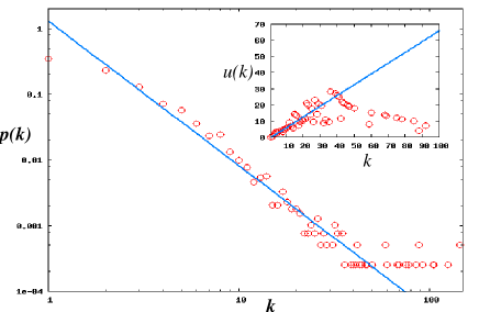
Figure 1: Degree distribution for the PPI network for Saccharomyces Cerevisiae PPI-Yeast . The evolution rule $u(k)$ derived using (16) is shown in the inset. The solid line here (inset) is a linear fit $u(k)=k-.8$, for which one expects $p(k)\sim k^{-2.2}$. A solid line with slope $-2.2$ is drawn in the main figure to compare $p(k)$ with the theory.

Here, $\alpha$ appears as an multiplicative constant which can be dropped as it is irrelevant for the evaluation of $p(k)$. Eq. (16) provides an insight about a possible evolution rule for any real world network. For example we take protein-protein interaction (PPI) network for Saccharomyces Cerevisiae (yeast) PPI-Yeast . The largest connected part has $N=3930$ nodes and $M=7725$ links. The degree distribution of this network is shown in Fig. 1. The average degree of this network is $3.93$ which may be modeled using $h(m)=0.4\delta_{m,1}+0.234\delta_{m,2}+0.366\delta_{m,3}$. We evaluate $u(k)$ for this network (shown in the inset of Fig.1) using (16) which fits well with a linear function $u(k)=1.5(k-.8)$. Note that for this fitting we ignore large $k$ values as for these values, $p(k)$ is very small and sometimes $zero$ also. Corresponding degree distribution is now expected to be scale-free $p(k)\sim k^{-2.2}$, which is consistent with the observed distribution.

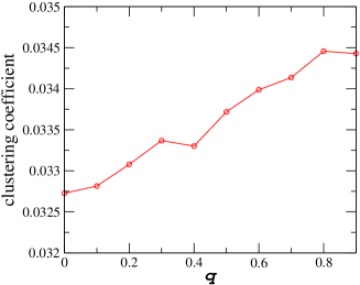
Figure 2: Clustering coefficient changes with a stochastic parameter $q$ (see text). Other parameters are $u(k)=k+0.5$, $N=1000$, $m=4$, $\eta(n)=q\delta_{n,1}+(1-q)\delta_{n,5}$ and the clustering coefficient is averaged over $1000$ realizations.

Now, we turn our attention to the other stochastic parameters $\eta(n)$, namely the distribution of number of nodes which join the network during each iteration time step $t$. We have seen in (10) that $\eta(n)$ do not alter the degree distribution. However they marginally affect correlations or the statistical properties of modular structures in the network. To illustrate this point, we generate a network with $u(k)=k+0.5$, $h(m)=\delta_{m,4}$ and $\eta(n)=q\delta_{n,1}+(1-q)\delta_{n,5}$, and measure the clustering coefficient for different $q$. As explained in the Fig. (2), we find that the clustering coefficient changes only marginally with $q$.

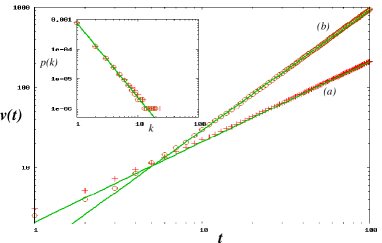
Figure 3: Log scale plot of $v(t)$ for two different cases : (a) $\eta(n)=0.6\delta_{1,n}+0.4\delta_{2,n}$ and (b) $n(t)=\sqrt{t}$. It is expected from (4) and (9) that $v(t)$ is linear in first case, whereas for (b) $v(t)\sim t^{3/2}$. Solid lines with slope $1$ and $1.5$ are drawn for comparison. For both cases, $u(k)=k-.5$ and $m=1$ and averaging is done over $1000$ realizations. The degree distribution $p(k)\sim k^{-2.5}$ (inset) is identical for both cases.

Our analysis here rely on the fact that Eq. (6) holds for large networks (as $t\to\infty$). Let us check the validity of (6) in details. From (9) it is clear that $v(t)$ is proportional to $N(t)$ which can be obtained from (4). First, we numerically evaluate $v(t)$ for few different networks and compare them with the theoretical results (4). If the number of new nodes $n$ is a stochastic variable then $N(t)=\bar{n}t+2$, is linear. However one can introduce an explicit time dependence in $n$ to get non-linear $N(t)$. For example, if $n(t)=\sqrt{t}$ we have $N(t)=t^{3/2}+2$ and thus $v(t)\propto t^{3/2}$. In figure (3) we plot numerically measured $v(t)$ in log scale for two different cases; (a) $n=0.6\delta_{n,1}+0.4\delta_{n,2}$ and (b) $n(t)=\sqrt{t}$, both agree well with (4). Although $N(t)$ is quite different, $p(k)$ (shown in the inset) was found to be same as expected. For both the cases evolution rule is $u(k)=k-.5$ and thus we have $p(k)\sim k^{-2.5}$. To conclude, Eq. (6) holds quite well after as few as ($t\sim 10$) iterations. For large networks, the number of nodes which join in first few iteration steps is vanishingly small as compared to the size of the network, hence do not affect the network properties.

In summary, we introduce a generic model of stochastically growing network and show that this model can easily be mapped to the ZRP and thus enabling us to derive an exact relation between the degree distribution of network and its evolution function. This relation can be used to derive analytical form of the degree distribution for any arbitrary evolution rule and conversely for a given network data we can infer about a possible evolution rule. Our evolution rule produce exact degree distribution, as obtained from the given network data, even for small $k$ values. We demonstrate this by taking example of a real world PPI networks and deriving a possible evolution rule to this network.

Based on our exact calculations we expect to get the better understanding of the the evolution of real world networks. Also, since ZRP is exactly solvable, mapping of ZRP with network growth models, opens up a platform to study the interplay between evolution rules and steady state degree distribution.

One of us (PKM) acknowledges MPIPKS for the hospitality and the support.

References

- (1) S. H. Strogatz, Nature 410, 268 (2001).
- (2) R. Albert and A.-L. Barabási, Rev. Mod. Phys. 74, 47 (2002) and references therein.
- (3) M. Girvan and M. E. J. Newman, Proc. Natl. Acad. Sci. USA 99, 7821 (2002); A. Clauset, M. E. J. Newman, and C. Moore, Phys. Rev. E 70, 066111 (2004); M. E. J. Newman, Social Networks 27, 39 (2005); M. E. J. Newman, Proc. Natl. Acad. Sci. USA 103, 8577 (2006).
- (4) R. Guimerá and L. A. N. Amaral, Nature 433, 895 (2005).
- (5) L. da. F. Costa, F. A. Rodrigues, G. Travieso and P. Villas Boas, Advances in Physics 56, 167 (2007).
- (6) P. Erdös and A. Rényi, Publ. Math. Inst. Hungar. Acad. Sci. 5, 17 (1960).
- (7) R. Albert, H. Jeong and A. -L. Barabási, Nature 401 130 (1999).
- (8) H. Jeong, B. Tombor, R. Albert, Z. N. Oltvai and A.-L. Barabási, Nature, 407, 651 (2000).
- (9) A.-L. Barabási and R. Albert, Science 286, 509 (1999); A.-L. Barabási, R. Albert and H. Jeong, Physica A 272 173 (1999).
- (10) S. N. Dorogovtsev and J. F. F. Mended, Phys. Rev. E 62, 1842 (2000).
- (11) P. L. Krapivsky, S. Redner and F. Leyvraz, Phys. Rev. Lett. 85, 4629 (2000).
- (12) D. J. Watts and S. H. Strogatz, Nature 440, 393 (1998).
- (13) E. Ravsaz, A. L. Somera, D. A. Mongru, Z. N. Oltavi and A.-L. Barabási, Science 297 1551 (2002); R. Guimerá and L. A. N. Amaral, Nature 433, 895 (2005).
- (14) V. Spirin and L. A. Mirny, Proc. Natl. Acad. Sci. USA 100 12123 (2003)
- (15) S. Maslov and K. Sneppen, Science 296 910 (2002).
- (16) R. Milo, S. Itzkovitz, N. Kashtan, R. Levitt, S. Shen-Orr, I. Ayzenshat, M. Sheffer and U. Alon, Science 303 1538 (2004)
- (17) R. Milo, S. Shen-Orr, S. Itzkovitz, N. Kashtan, D. Chklovskii and U. Alon, Science 298 824 (2002).
- (18) R. J. Williams and N. D. Martinez, Nature 404 180 (2000).
- (19) P. L. Krapivsky and S. Redner, Phys. Rev. E 63, 066123 (2001).
- (20) I. Ispolatov, P. L. Krapivsky, I. Mazo and A. Yuryev, New Journal of Physics 7, 145 (2005).
- (21) H. Rozenfeld and D. ben-Avraham, Phys. Rev. E 70, 056107 (2004).
- (22) For a review on ZRP see, M R Evans and T Hanney, J. Phys. A: Math. Gen. 38, R195 (2005).
- (23) S. N. Dorogovtsev, J. F. F. Mendes and A. N. Samukhin, Phys. Rev. Lett, 85, 4633 (2000).
- (24) S. N. Dorogovtsev and J. F. F. Mendes, Phys. Rev. E 63, 056125 (2001).
- (25) Data published by COSIN Project Group, http://www.cosin.org/extra/data/proteins/