Quantum Teleportation and Von Neumann Entropy

Abstract

The single qubit quantum teleportation (sender and receiver are Alice and Bob respectively) is analyzed from the aspect of the quantum information theories. The various quantum entropies are computed at each stage, which ensures the emergence of the entangled states in the intermediate step. The mutual information $S(B:C)$ becomes non-zero before performing quantum measurement, which seems to be consistent to the original purpose of the quantum teleportation. It is shown that if the teleported state $|\psi\rangle$ is near the computational basis, the quantum measurement in $C$-system is dominantly responsible for the joint entropy $S(A,C)$ at the final stage. If, however, $|\psi\rangle$ is far from the computational basis, this dominant responsibility is moved into the quantum measurement of system $A$. A possible extension of our results are briefly discussed.

I Introduction

Figure 1: Quantum circuit for teleporting a qubit $|\psi\rangle$. The two top lines represent Alice’s system and the bottom line is Bob’s system.

It is generally believed that Nature is governed by quantum mechanicsfeynman65 . Based on this fact, Feynman suggestedfeynman82 ; feynman86 about three decades ago that the computer which obeys the quantum mechanical law can be made in the future. Ten years later after Feynman suggestion P. W. Shorshor94 has shown that the computer Feynman pointed out, i.e. quantum computer, enhances drastically the computational ability in certain mathematical problems. Especially, Shor showed that the discrete logarithm and large integer factoring problems can be computed within polynomial time in the quantum computer. Recently, this factoring algorithm is experimentally realized in NMRvander01 and opticallu07 experiments. Since the efficient factoring algorithm is highly important in modern cryptography, Shor’s factoring algorithm supports a strong motivation on current flurry of activity in this subject. Furthermore, the recent active research on quantum computer provides a deep understanding in quantum mechanics, and as a result it yields a new branch of physics called quantum informationnielsen00 .

Although the quantum computation and quantum information theories are important in the aspect of industrial issue, they also gives an new insight in the purely theoretical aspects. In theoretical physics, as well-known, one of the most important and long-standing problem is how to understand and formulate the quantum gravity. The most important effect of the quantum gravity, which still we do not fully understand, is an information loss problem in black hole physicshawk76 . Recent development of the quantum information theories may shed light on the new avenue to understand this highly important and fundamantal problemsloss .

In this paper we would like to examine the quantum teleportationbennett93 from the viewpoint of the quantum entropy called von Neumann entropy. The quantum circuit for the one qubit teleportation is given in Fig. 1. The two top lines in Fig. 1 are Alice’s system and the bottom line is Bob’s system. The main purpose of the quantum teleportation is to send the unknown quantum state $|\psi\rangle=a|0\rangle+b|1\rangle$ from Alice to Bob. The state vector for each stage before Alice performs quantum measurement can be easily read from Fig. 1 as following:

$$|CAB\rangle=\frac{1}{\sqrt{2}}\left[a(|000\rangle+|010\rangle)+b(|100\rangle+|110\rangle)\right]\hskip 14.22636pt\mbox{(at stage 1)}$$ (1)

$$|CAB\rangle=\frac{1}{\sqrt{2}}\left[a(|000\rangle+|011\rangle)+b(|100\rangle+|111\rangle)\right]\hskip 14.22636pt\mbox{(at stage 2)}$$

$$|CAB\rangle=\frac{1}{\sqrt{2}}\left[a(|000\rangle+|011\rangle)+b(|101\rangle+|110\rangle)\right]\hskip 14.22636pt\mbox{(at stage 3)}$$

$$|CAB\rangle=\frac{1}{2}\bigg{[}a(|000\rangle+|011\rangle+|100\rangle+|111\rangle)$$

$$\hskip 85.35826pt+b(|001\rangle+|010\rangle-|101\rangle-|110\rangle)\bigg{]}.\hskip 14.22636pt\mbox{(at stage 4)}$$

The quantum teleportation is possible if one uses the various pecular properties of the EPR maximally entangled states which have no counterpart in the classical channel. In fact we can show that the state vector of the AB sub-system at stage “2” is

$$|AB\rangle=\frac{1}{\sqrt{2}}\left(|00\rangle+|11\rangle\right)$$ (2)

which is one of four EPR states in two qubit system. After stage “4” Alice performs a quantum measurement in the computational basis. Thus the measurement outcome should be one of ($C=0,A=0$), ($C=0,A=1$), ($C=1,A=0$), and ($C=1,A=1$). To complete the teleportation Alice should notify Bob of the measurement result via the classical channel. If Alice’s measurement result is ($C=M_{1}$, $A=M_{2}$), Bob should operate $Z^{M_{1}}X^{M_{2}}$ to his state where

$$X=\left(\begin{array}[]{cc}0&1\\ 1&0\end{array}\right),\hskip 28.45274ptY=\left(\begin{array}[]{cc}0&-i\\ i&0\end{array}\right),\hskip 28.45274ptZ=\left(\begin{array}[]{cc}1&0\\ 0&-1\end{array}\right).$$ (9)

Then, as a result, Bob’s state vector reduces to $|B\rangle=a|0\rangle+b|1\rangle$. Thus the state $|\psi\rangle$ is completely teleported to Bob. This is a quantum algorithm for the single qubit quantum teleportation.

The single qubit quantum teleportation is experimentally realized in opticsbouwmeester97 ; furu98 , nuclear magnetic resonanceniel98 and ion trap experimentriebe07 . More recently, the quantum algorithm for the two qubit teleportation is developedyan05 via the optimal POVM measurement performed by Bob.

As stated above we would like to examine the single qubit quantum teleportation algorithm in this paper by computing the various quantum entropies at all stages. This paper is origanized as follows. In section II we compute the von Neumann entropies, joint entropies, relative entropies, conditional entropies and mutual information at each stage before quantum measurement. It is shown that the local Hadamard gate does not give any effect in quantum entropy. The mutual information $S(B:C)$ becomes non-zero at stage “3” and “4”. This means that the partial information on $|\psi\rangle$ is moved to Bob, which is consistent with the original purpose of the teleportation. Several conditional entropies become negative, which indicates the appearance of the entangled statesnielsen00 . In section III we compute the various quantum entropies at stage “5”, where Alice performed her measurement but still has not informed Bob of her measurement result. This situation can be described differently as following: although Alice performs her projective measurement, for some reason she lost the record of her measurement result. Then it is physically reasonable to assume that the density operator for the joint system CAB is the averaged value produced via quantum measurement. It is shown that the joint and conditional entropies increase due to the projective measurement while mutual information decreases. The physical reason for the decrease of the mutual information is discussed in this section. In section IV we introduce two different intermediate stages between stage “4” and “5” to examine the effect of the quantum measurement on quantum entropy. In section V a brief conclusion is given.

II Single-qubit Teleportation: before measurement

In this section we would like to compute various quantities derived from von Neumann’s entropy defined

$$S(\rho)\equiv-Tr\left(\rho\log\rho\right)$$ (10)

where $\rho$ is a density operator of a given quantum system. Especially, in this section, we consider only stage $``1^{\prime\prime}$, $``2^{\prime\prime}$, $``3^{\prime\prime}$ and $``4^{\prime\prime}$ in Fig. 1. The stage $``5^{\prime\prime}$(stage after quantum measurement performed by Alice) will be explored in the next section. Since the computational technique for each stage is similar, we will show the calculational procedure explicitly only at stage $``3^{\prime\prime}$ and the results for each level will be summarized in Table I, II and III.

Using Eq.(1) it is easy to show that the density operator $\rho^{CAB}$ for the joint system CAB becomes

$$\rho^{CAB}\equiv|CAB\rangle\langle CAB|=\frac{1}{2}\left(\begin{array}[]{cccccccc}|a|^{2}&0&0&|a|^{2}&0&ab^{*}&ab^{*}&0\\ 0&0&0&0&0&0&0&0\\ 0&0&0&0&0&0&0&0\\ |a|^{2}&0&0&|a|^{2}&0&ab^{*}&ab^{*}&0\\ 0&0&0&0&0&0&0&0\\ a^{*}b&0&0&a^{*}b&0&|b|^{2}&|b|^{2}&0\\ a^{*}b&0&0&a^{*}b&0&|b|^{2}&|b|^{2}&0\\ 0&0&0&0&0&0&0&0\end{array}\right).$$ (19)

Since $\rho^{CAB}$ is pure state and von Neumann entropy for pure state is always zeronielsen00 , one can conclude

$$S(C,A,B)=0.$$ (20)

Taking partial trace for Bob’s system, one can directly compute $\rho^{CA}$, the density operator for the CA joint system, whose explicit expression is

$$\rho^{CA}=Tr_{B}\rho^{CAB}=\frac{1}{2}\left(\begin{array}[]{cccc}|a|^{2}&0&0&ab^{*}\\ 0&|a|^{2}&ab^{*}&0\\ 0&a^{*}b&|b|^{2}&0\\ a^{*}b&0&0&|b|^{2}\end{array}\right).$$ (25)

Since $Tr(\rho^{CA})^{2}=1/2\neq 1$, $\rho^{CA}$ is a mixed state. It is easy to show that $\rho^{CA}$ has eigenvalues $\lambda_{CA}=\{1/2,1/2,0,0\}$. Since von Neumann entropy equals to the classical Shannon entropy if the eigenvalues of the density operator are regarded as the probability distribution, the quantum entropy reduces to

$$S(C,A)\equiv-\sum_{i}\lambda_{i}\log\lambda_{i}=1.$$ (26)

By same way it is easy to show that $\rho^{CB}=\rho^{CA}$ and

$$\rho^{AB}=Tr_{C}\rho^{CAB}=\frac{1}{2}\left(\begin{array}[]{cccc}|a|^{2}&0&0&|a|^{2}\\ 0&|b|^{2}&|b|^{2}&0\\ 0&|b|^{2}&|b|^{2}&0\\ |a|^{2}&0&0&|a|^{2}\end{array}\right)$$ (31)

with

$$S(C,B)=1,\hskip 28.45274ptS(A,B)=-|a|^{2}\log|a|^{2}-|b|^{2}\log|b|^{2}.$$ (32)

Tracing out again, one can derive the density operators for the single qubit systems

$$\rho^{C}=\left(\begin{array}[]{cc}|a|^{2}&0\\ 0&|b|^{2}\end{array}\right),\hskip 28.45274pt\rho^{A}=\rho^{B}=\frac{1}{2}\left(\begin{array}[]{cc}1&0\\ 0&1\end{array}\right)$$ (37)

with

$$S(C)=-|a|^{2}\log|a|^{2}-|b|^{2}\log|b|^{2},\hskip 28.45274ptS(A)=S(B)=1.$$ (38)

Eq.(37) implies that $\rho^{A}$ and $\rho^{B}$ are completely mixed states.

state	stage 1	stage 2	stage 3,4	stage 5
$\rho^{CAB}$	(P,P)	(P,E)	(P,E)	(M,E)
$\rho^{CA}$	(P,P)	(M,P)	(M,E)	(completely M,P)
$\rho^{CB}$	(P,P)	(M,P)	(M,E)	(M,E)
$\rho^{AB}$	(P,P)	(P,E)	(M,E)	(M,E)
$\rho^{C}$	P	P	M	completely M
$\rho^{A}$	P	completely M	completely M	completely M
$\rho^{B}$	P	completely M	completely M	completely M

Table I: The properties of the density operators at each stage. The P and M in first position in parenthesis denote pure and mixed respectively. The P and E in second position stand for product and entangled respectively.

Using the definitions of mutual information $S(A:B)\equiv S(A)+S(B)-S(A,B)$ and conditional entropy $S(A|B)\equiv S(A,B)-S(B)$ one can compute the various quantities summarized in Table II.

The relative entropy defined

$$S(\rho||\sigma)\equiv Tr\left(\rho\log\rho\right)-Tr\left(\rho\log\sigma\right)=-S(\rho)-Tr\left(\rho\log\sigma\right)$$ (39)

also can be computed explicitly. Using

$$\log\rho^{C}=\left(\begin{array}[]{cc}\log|a|^{2}&0\\ 0&\log|b|^{2}\end{array}\right),\hskip 28.45274pt\log\rho^{A}=\log\rho^{B}=\left(\begin{array}[]{cc}-1&0\\ 0&-1\end{array}\right),$$ (44)

one can easily show

$$S(\rho^{C}||\rho^{A})=S(\rho^{C}||\rho^{B})=1+|a|^{2}\log|a|^{2}+|b|^{2}\log|b|^{2}$$ (45)

$$S(\rho^{A}||\rho^{C})=S(\rho^{B}||\rho^{C})=-\log(2|a||b|)$$

$$S(\rho^{A}||\rho^{B})=S(\rho^{B}||\rho^{A})=0.$$

The relative entropy for other stages is summarized at Table III. Table III shows that the relative entropy is always non-negative, which is known as Klein’s inequality. Another point Table III indicates is that the relative entropy sometimes becomes infinity due to $\log 0$. This is because of the non-trivial intersection of support of $\rho$ with kernel of $\sigma$.

In order to check whether the states are entangled or not, we compare the tensor product of the component states with the corresponding joint state. At stage “3” one can show easily

$$\rho^{AB}\neq\rho^{A}\otimes\rho^{B}\hskip 28.45274pt\rho^{CA}\neq\rho^{C}\otimes\rho^{A}$$ (46)

$$\rho^{CB}\neq\rho^{C}\otimes\rho^{B}\hskip 28.45274pt\rho^{CAB}\neq\rho^{C}\otimes\rho^{A}\otimes\rho^{B}$$

which indicates that all joint states are entangled at this stage. The answer of the question whether the given states are entangled or product, and mixed or pure at each stage is summarized at Table I. In Table I (P,E) means “pure and entangled” and (M,P) stands for “mixed and product”. Therefore Table I shows that the quantum teleportation generally converts “pure and product” at stage “1” to “mixed and entangled” at stage “4” for the joint system and “pure” at stage “1” to “completely mixed” at stage “4” for single-qubit component systems.

entropy	stage 1	stage 2	stage 3, 4	stage 5
$S(A,B,C)$	$0$	$0$	$0$	$2$
$S(A)$	$0$	$1$	$1$	$1$
$S(B)$	$0$	$1$	$1$	$1$
$S(C)$	$0$	$0$	$-|a|^{2}\log|a|^{2}-|b|^{2}\log|b|^{2}$	$1$
$S(A,B)$	$0$	$0$	$-|a|^{2}\log|a|^{2}-|b|^{2}\log|b|^{2}$	$1-|a|^{2}\log|a|^{2}-|b|^{2}\log|b|^{2}$
$S(A,C)$	$0$	$1$	$1$	$2$
$S(B,C)$	$0$	$1$	$1$	$2-\frac{1}{2}\log(1-u^{2})-\frac{u}{2}\log\frac{1+u}{1-u}$
$S(A:B)$	$0$	$2$	$2+|a|^{2}\log|a|^{2}+|b|^{2}\log|b|^{2}$	$1+|a|^{2}\log|a|^{2}+|b|^{2}\log|b|^{2}$
$S(B:C)$	$0$	$0$	$-|a|^{2}\log|a|^{2}-|b|^{2}\log|b|^{2}$	$\frac{1}{2}\log(1-u^{2})+\frac{u}{2}\log\frac{1+u}{1-u}$
$S(A:C)$	$0$	$0$	$-|a|^{2}\log|a|^{2}-|b|^{2}\log|b|^{2}$	$0$
$S(A|B)$	$0$	$-1$	$-1-|a|^{2}\log|a|^{2}-|b|^{2}\log|b|^{2}$	$-|a|^{2}\log|a|^{2}-|b|^{2}\log|b|^{2}$
$S(A|C)$	$0$	$1$	$1+|a|^{2}\log|a|^{2}+|b|^{2}\log|b|^{2}$	$1$
$S(B|C)$	$0$	$1$	$1+|a|^{2}\log|a|^{2}+|b|^{2}\log|b|^{2}$	$1-\frac{1}{2}\log(1-u^{2})-\frac{u}{2}\log\frac{1+u}{1-u}$
$S(B|A)$	$0$	$-1$	$-1-|a|^{2}\log|a|^{2}-|b|^{2}\log|b|^{2}$	$-|a|^{2}\log|a|^{2}-|b|^{2}\log|b|^{2}$
$S(C|A)$	$0$	$0$	$0$	$1$
$S(C|B)$	$0$	$0$	$0$	$1-\frac{1}{2}\log(1-u^{2})-\frac{u}{2}\log\frac{1+u}{1-u}$

Table II: Various quantum entropy at each stage ($u\equiv ab^{*}+a^{*}b$).

relative entropy	stage 1	stage 2	stage 3, 4	stage 5
$S(\rho^{C}||\rho^{A})$	$-\frac{1}{2}(\log 0)(1-u)$	$1$	$1+|a|^{2}\log|a|^{2}+|b|^{2}\log|b|^{2}$	$0$
$S(\rho^{A}||\rho^{C})$	$-\frac{1}{2}(\log 0)(1-u)$	$-1-\frac{1}{2}(\log 0)$	$-\log(2|a||b|)$	$0$
$S(\rho^{C}||\rho^{B})$	$-(\log 0)|b|^{2}$	$1$	$1+|a|^{2}\log|a|^{2}+|b|^{2}\log|b|^{2}$	$0$
$S(\rho^{B}||\rho^{C})$	$-(\log 0)|b|^{2}$	$-1-\frac{1}{2}(\log 0)$	$-\log(2|a||b|)$	$0$
$S(\rho^{A}||\rho^{B})$	$-\frac{1}{2}(\log 0)$	$0$	$0$	$0$
$S(\rho^{B}||\rho^{A})$	$-\frac{1}{2}(\log 0)$	$0$	$0$	$0$

Table III: Relative entropy at each stage ($u\equiv ab^{*}+a^{*}b$).

Now we would like to discuss Table II briefly. As is well-known, the original purpose of the quantum teleportation is for Alice(A) to send $\psi\rangle=a|0\rangle+b|1\rangle$ in C-system to Bob(B) using a Bell state $(|00\rangle+|11\rangle)/\sqrt{2}$, which is shared by Alice and Bob at stage “2”. That is why the mutual information $S(B:C)$ between B and C becomes non-zero at stage“3” and “4”. Table II also shows that several conditional entropies become negative, which indicates the emergence of the entangled statesnielsen00 . Another point we would like to stress is the fact that all joint entropies increase when stage is moved from “4” to “5”. Since level “5” is a stage just after the quantum measurement performed by Alice, this fact reflects that the projective measurements generally increase the quantum entropynielsen00 . In the next section we will discuss how the quantities at stage “5” are computed.

III Single-qubit Teleportation: after measurement

The stage “5” is just after Alice has performed the quantum measurement but just before Bob has learned the measurement result. We can describe the situation of the stage “5” differently as following. Firstly, Alice performed the quantum measurement at the computational besis $\{|00\rangle,|01\rangle,|10\rangle,|11\rangle\}$ of the joint CA-system. In order to compute the probability $P(C,A)$ for the measurement result, we need an reduced density operator $\rho^{CA}$ at stage “4” which is

$$\left(\rho^{CA}\right)_{4}=\frac{1}{4}\left(\begin{array}[]{cccc}1&ab^{*}+a^{*}b&|a|^{2}-|b|^{2}&-(ab^{*}-a^{*}b)\\ ab^{*}+a^{*}b&1&-(ab^{*}-a^{*}b)&|a|^{2}-|b|^{2}\\ |a|^{2}-|b|^{2}&ab^{*}-a^{*}b&1&-(ab^{*}+a^{*}b)\\ ab^{*}-a^{*}b&|a|^{2}-|b|^{2}&-(ab^{*}+a^{*}b)&1\\ \end{array}\right).$$ (51)

Thus the probability $P(0,0)$ for Alice to get $C=0$ and $A=0$ is

$$P(0,0)=Tr\left[|00\rangle\langle 00|\left(\rho^{CA}\right)_{4}\right]=\frac{1}{4}.$$ (52)

By same way one can show easily $P(0,1)=P(1,0)=P(1,1)=1/4$.

$\scriptstyle P(C.A)$	$\scriptstyle P(0,0)=\frac{1}{4}$	$\scriptstyle P(0,1)=\frac{1}{4}$	$\scriptstyle P(1,0)=\frac{1}{4}$	$\scriptstyle P(1,1)=\frac{1}{4}$
$\scriptstyle\rho^{\scriptstyle CAB}$	$\scriptstyle|00\rangle\langle 00|\otimes\left(\begin{array}[]{cc}\scriptstyle|a|^{2}&\scriptstyle ab^{*}\\ \scriptstyle a^{*}b&\scriptstyle|b|^{2}\end{array}\right)$	$\scriptstyle|01\rangle\langle 01|\otimes\left(\begin{array}[]{cc}|\scriptstyle b|^{2}&\scriptstyle a^{*}b\\ \scriptstyle ab^{*}&\scriptstyle|a|^{2}\end{array}\right)$	$\scriptstyle|10\rangle\langle 10|\otimes\left(\begin{array}[]{cc}\scriptstyle|a|^{2}&\scriptstyle-ab^{*}\\ \scriptstyle-a^{*}b&\scriptstyle|b|^{2}\end{array}\right)$	$\scriptstyle|11\rangle\langle 11|\otimes\left(\begin{array}[]{cc}\scriptstyle|b|^{2}&\scriptstyle-a^{*}b\\ \scriptstyle-ab^{*}&\scriptstyle|a|^{2}\end{array}\right)$

Table IV: The probability distribution for the projective measurement performed by Alice and the corresponding joint density operator $\rho^{CAB}$ at stage “5”.

In order to compute $\rho^{CAB}$ at stage “5” we need $\rho^{CAB}$ at stage “4” which is

$$\rho_{4}^{CAB}=\frac{1}{4}\Bigg{[}|00\rangle\langle 00|\otimes(a|0\rangle+b|1\rangle)(a^{*}\langle 0|+b^{*}\langle 1|)$$ (53)

$$+|01\rangle\langle 01|\otimes(b|0\rangle+a|1\rangle)(b^{*}\langle 0|+a^{*}\langle 1|)+|10\rangle\langle 10|\otimes(a|0\rangle-b|1\rangle)(a^{*}\langle 0|-b^{*}\langle 1|)$$

$$\hskip 56.9055pt+|11\rangle\langle 11|\otimes(-b|0\rangle+a|1\rangle)(-b^{*}\langle 0|+a^{*}\langle 1|)+\cdots\Bigg{]}$$

where $\cdots$ denotes the off-diagonal part in the joint CA-system. Thus if Alice gets $C=A=0$ in the projective measurement, $\rho^{CAB}$ at stage “5” reduces to

$$\rho_{0,0}^{CAB}=\frac{1}{P(0,0)}(|00\rangle\langle 00|)\rho_{4}^{CAB}(|00\rangle\langle 00|)=(|00\rangle\langle 00|)\otimes\left(\begin{array}[]{cc}|a|^{2}&ab^{*}\\ a^{*}b&|b|^{2}\end{array}\right).$$ (56)

If Alice gets different measurement results, we have, of course, different $\rho^{CAB}$ at stage “5”. The possible measurement results and the corresponding $\rho^{CAB}$ at stage “5” is summarized at Table IV.

Since Alice does not inform the measurement result to Bob yet at level “5”, the density operator at this stage should be same with the density operator for the case that Alice lost, for some reason, her record of the measurement result. In the latter case it is reasonable to conjecture $\rho^{CAB}$ as an average value as following:

$$\rho^{CAB}=\frac{1}{4}(|00\rangle\langle 00|)\otimes\left(\begin{array}[]{cc}|a|^{2}&ab^{*}\\ a^{*}b&|b|^{2}\end{array}\right)+\frac{1}{4}(|01\rangle\langle 01|)\otimes\left(\begin{array}[]{cc}|b|^{2}&a*b\\ ab^{*}&|a|^{2}\end{array}\right)$$ (61)

$$\hskip 28.45274pt+\frac{1}{4}(|10\rangle\langle 10|)\otimes\left(\begin{array}[]{cc}|a|^{2}&-ab^{*}\\ -a^{*}b&|b|^{2}\end{array}\right)+\frac{1}{4}(|11\rangle\langle 11|)\otimes\left(\begin{array}[]{cc}|b|^{2}&-a*b\\ -ab^{*}&|a|^{2}\end{array}\right).$$ (66)

Since $Tr(\rho^{CAB})^{2}=1/4$, it is a mixed state. Its eigenvalues are $\{1/4,0\}$ with four-fold degeneracies respectively, and therefore the corresponding von Neumann entropy is

$$S(C,A,B)=2.$$ (67)

Tracing out A, B, and C respectively, one can easily construct

$$\rho^{CA}=\frac{I}{4}\hskip 28.45274pt\rho^{CB}=\frac{1}{4}\left(\begin{array}[]{cccc}1&u&0&0\\ u&1&0&0\\ 0&0&1&-u\\ 0&0&-u&1\end{array}\right)\hskip 28.45274pt\rho^{AB}=\frac{1}{2}\left(\begin{array}[]{cccc}|a|^{2}&0&0&0\\ 0&|b|^{2}&0&0\\ 0&0&|b|^{2}&0\\ 0&0&0&|a|^{2}\end{array}\right)$$ (76)

where $I$ is unit matrix and $u=ab^{*}+a^{*}b$. It is worthwhile noting that $\rho^{CA}$ becomes completely mixed state in thi stage. This means that Alice’s knowledge on $|\psi\rangle$ becomes completely mixed out through the quantum measurement. Computing the eigenvalues, one can easily compute the corresponding entropies which is explicitly given at Table II. Tracing out again one can also show that the density operators for all single-qubit systems become completely mixed:

$$\rho^{C}=\rho^{A}=\rho^{B}=\frac{I}{2}.$$ (77)

This fact indicates that Bob cannot conjecture the state $|\psi\rangle$ without the classical channel described in Fig. 1. This fact reconciles the quantum mechanics with the theory of relativity in the faster-than-light-communication.

Table II shows that all joint entropies at stage “5” increase compared to those at stage “4”. This fact reflects the well-known fact that the projective measurement increases the quantum entropy. In spite of the projective measurement, however, $S(A)$ and $S(B)$ remains same at both stages. This is because that at stage “2” AB system becomes maximally entangled and therefore the von Neumenn entropies for the component systems become maximum. Thus it is impossible to increase the entropies although Alice performs the projective measurement between stage “4” and “5”.

Another remarkable point in Table II is that the mutual informations decrease at stage “5” compared to stage “4”. This decreasing behavior is obvious for $S(A:B)$ and $S(A:C)$ but not manifest for $S(B:C)$. To show that $S(B:C)$ decreases too we note

$$S(B:C)=\left\{\begin{array}[]{cc}-r^{2}\log r^{2}-(1-r^{2})\log(1-r^{2})&\hskip 14.22636pt\mbox{at stage ``4''}\\ \frac{1}{2}\log(1-u^{2})+\frac{u}{2}\log\frac{1+u}{1-u}&\hskip 14.22636pt\mbox{at stage ``5''}\end{array}\right.$$ (80)

where $u=2r\sqrt{1-r^{2}}\cos\theta$ with $r=|a|$ and $\theta=Arg(a)-Arg(b)$. Plotting together one can show that $S(B:C)$ at stage “4” is always larger than $S(B:C)$ at stage “5”. The decreasing behavior of the mutual information can be explained as follows. Note that $S(A:B)\equiv S(A)+S(B)-S(A,B)$. Since the state of AB-system is maximally entangled at stage “2”, $S(A)$ and $S(B)$ become maximized before quantum measurement performed by Alice. However, the joint AB-system is two-qubit system, the maximum of $S(A,B)$ is two, and the joint entropy has a room to increase by the projective measurement. As a result, therefore, the mutual informations exhibit decreasing behavior at stage “5”. Finally all of the conditional entropies increase at stage “5”. This can be explained too using a similar argument.

IV Quantum Measurement Issue

Figure 2: Two different intermediate stages between stage “4” and stage “5”. These intermediate stages are introduced to examine the effect of quantum measurement in the change of quantum entropy.

In this section we would like to examine the issue on the effect of the quantum measurement in the change of quantum entropy. In order to explore this issue in detail we assume that Alice performs the quantum measurement for C and A systems in different time as shown in Fig. 2. Thus we have two different stages “4.5-1” and “4.5-2” between stage “4” and stage “5”.

Now we consider stage “4.5-1”, where the projective measurement is performed at the computational basis $\{(|0\rangle\langle 0|)_{C},(|1\rangle\langle 1|)_{C}\}$. In order to compute the probability for the measurement results $C=0$ or $C=1$ we need $\rho^{C}$ at stage “4”, which is

$$(\rho^{C})_{4}=\frac{1}{2}\left[|0\rangle\langle 0|+(|a|^{2}-|b|^{2})|0\rangle\langle 1|+(|a|^{2}-|b|^{2})|1\rangle\langle 0|+|1\rangle\langle 1|\right].$$ (81)

Thus the probabilities become

$$P(C=0)=Tr[|0\rangle\langle 0|(\rho^{C})_{4}]=\frac{1}{2}$$ (82)

$$P(C=1)=Tr[|1\rangle\langle 1|(\rho^{C})_{4}]=\frac{1}{2}.$$

When the quantum measurement yields C=0, the density operator for CAB joint system becomes

$$\rho_{0}^{CAB}=\frac{1}{P(C=0)}\left[(|0\rangle\langle 0|)_{C}\rho_{4}^{CAB}(|0\rangle\langle 0|)_{C}\right]$$ (83)

where $\rho_{4}^{CAB}$ is density operator for CAB system at stage “4”. By same way it is straightforward to compute $\rho_{1}^{CAB}$, i.e. the density operator for CAB system when Alice gets C=1, which is

$$\rho_{1}^{CAB}=\frac{1}{P(C=1)}\left[(|1\rangle\langle 1|)_{C}\rho_{4}^{CAB}(|1\rangle\langle 1|)_{C}\right].$$ (84)

If Alice lost the record of her measurement result, the density operator reduces to its expectation value

$$\rho^{CAB}=P(C=0)\rho_{0}^{CAB}+P(C=1)\rho_{1}^{CAB}.$$ (85)

Once the density operator for total system is obtained, it is easy to compute the density operator for the sub-systems by making use of the partial trace appropriately. Then one can compute the von Neumann entropies easily. Of course similar computational procedure can be applied to compute the quantum entropy at stage “4.5-2”. The various quantum entropies at stage “4.5-1” and “4.5-2” are summarized at Table V when Alice lost her record of the measurement result.

	stage “4.5-1”	stage “4.5-2”
$S(A,B,C)$	$1$	$1$
$S(A)$	$1$	$1$
$S(B)$	$1$	$1$
$S(C)$	$1$	$-|a|^{2}\log|a|^{2}-|b|^{2}\log|b|^{2}$
$S(A,B)$	$-|a|^{2}\log|a|^{2}-|b|^{2}\log|b|^{2}$	$1-|a|^{2}\log|a|^{2}-|b|^{2}\log|b|^{2}$
$S(A,C)$	$2-\frac{1}{2}\log(1-u^{2})-\frac{u}{2}\log\frac{1+u}{1-u}$	$1-|a|^{2}\log|a|^{2}-|b|^{2}\log|b|^{2}$
$S(B,C)$	$2-\frac{1}{2}\log(1-u^{2})-\frac{u}{2}\log\frac{1+u}{1-u}$	$1$

Table V:Various quantum entropy at stage “4.5-1” and stage “4.5-2” ($u\equiv ab^{*}+a^{*}b$).

The quantum entropies in the intermediate stages have several properties. For example, the quantum state in the C-system becomes completely mixed at stage “4.5-1”, which is same with that of stage “5”. However, at stage “4.5-2” $S(C)$ is same with that of stage “4”. This fact indicates that measuring C performed by Alice is responsible for the change of $S(C)$ between stage “4” and “5”. Same and converse situations occur in $S(B,C)$ and $S(A,B)$ respectively. The only one which has non-trivial value in the intermediate stage is $S(A,C)$. Of course $S(A,C)$ in the intermediate stages “4.5-1” and “4.5-2” are between $1$ and $2$, where the former is $S(A,C)$ at stage “4” while the latter is at stage “5”. Defining $r=|a|$ and $\theta=Arg(a)-Arg(b)$ again, one can plot $S(A,C)$ which is given in Fig. 3.

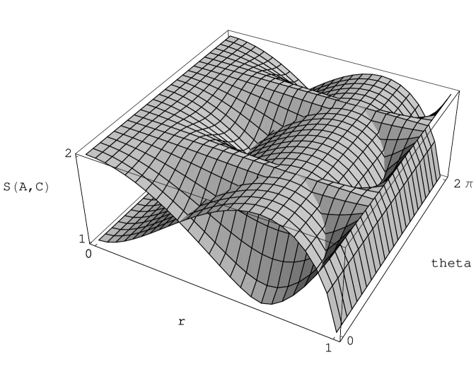
Figure 3: Plot of joint entropy $S(A,C)$ at intermediate stages “4.5-1” and “4.5-2” with varying $0\leq r\equiv|a|\leq 1$ and $0\leq\theta\equiv Arg(a)-Arg(b)\leq 2\pi$. This figure indicates that if $|\psi\rangle$ is close to the computational basis ($r\sim 0$ or $r\sim 1$), $S(A,C)$ in the stage “4.5-1” is much larger than that in the stage “4.5-2” while converse situation occurs when $|\psi\rangle$ is far from the computational basis.

Fig. 3 indicates that in the small $r$ and large $r$ region $S(A,C)$ in the stage “4.5-1” is much larger than that in stage “4.5-2”. However, in the intermediate range $S(A,C)$ in the stage “4.5-2” becomes much larger. This means that if $|\psi\rangle$ is close to the computational basis, measuring C is dominantly responsible for $S(A,C)$ at stage “5”. If, however, $|\psi\rangle$ is far from the computational basis, this responsibility is changed into the measurment of system A.

V conclusion

In this paper we have analyzed the single qubit quantum teleportation by computing the various quantum entropies at each stage of Fig. 1. Before quantum measurement performed by Alice between stage “4” and stage “5”, the von Neumann entropies, conditional entropies, relative entropies and mutual information are summarized in Table II and III. Table III shows that the relative entropy is always non-negative, which is well-known as Klein’s inequality. Therefore, the relative entropy can be regarded as a measure for distance between two different quantum states like trace distance or fidelity. Some relative entropies become infinity, which indicates the non-trivial intersection of the support of one quantum state with kernel of the other quantum state. Table II shows that the mutual information $S(B:C)$ becomes non-negative at stage “3” and “4”. This means that the partial information on $|\psi\rangle$ is transmitted to Bob, consistent with the original purpose of the quantum teleportation. Table II also shows that some conditional entropies become negative when the corresponding joint systems are in pure states. This fact indicates that the component systems are entangled. Of course there are many entangled states in sub-systems when the joint system is not in pure state. The properties of entangled or product, and pure or mixed for all systems are summarized in Table I.

At stage “5”, where Alice performs the projective measurement but she has not yet informed of the measurement result to Bob through classical channel, the state for the joint system CAB can be chosen as an average expectation value. In this case the state of total system CAB becomes mixed and entangled. The various quantum entropies are summarized at Table II and Table III. Table II shows that the joint and conditional entropies increase due to the projective measurement while the mutual information decreases. The reason for the decrease of the mutual information is discussed in section III.

Finally we have introduced two different intermediate stages “4.5-1” and “4.5-2” between stage “4” and “5” in Fig. 2 to examine the effect of the quantum measurement in the quantum entropies. The quantum entropies in these intermediate stages are summarized in Table V. Table V shows that all entropies except $S(A,C)$ are either one of corresponding entropies at stage “4” or stage “5”. The joint entropy $S(A,C)$ at stage “4.5-1” and “4.5-2” are plotted in Fig. 3. From this figure we can understand that if $|\psi\rangle$ is close to the computational basis, measuring $C$ is dominantly responsible for $S(A,C)$ at stage “5” while this dominant responsibility is changed into the measurement of $A$ if $|\psi\rangle$ is far from the computational basis.

It is of interest to extend our results to the quantum algorithm for the multi-qubit quantum teleportation. Also it seems to be interest to analyze the Shor’s factoring algorithmshor94 and Grover’s search algorithmgrover96 ; grover97 from the aspect of the quantum information theories. We hope to visit these issues in the near future.

Acknowledgement: This work was supported by the Kyungnam University Research Fund, 2006.

References

- (1) R. P. Feynman and A. R. Hibbs, Quantum Mechanics and Path Integrals (McGraw-Hill, New York, 1965).
- (2) R. P. Feynman, Simulating Physics with Computers, Int. J. Theor. Phys. 21 (1982) 467.
- (3) R. P. Feynman, Quantum Mechanical Computers, Found. Phys. 16 (1986) 507.
- (4) P. W. Shor, Algorithms for Quantum Computation: Discrete Logarithms and Factoring, Proc. 35th Annual Symposium on Foundations of Computer Science (1994) 124.
- (5) L. M. K. Vandersypen, M. Steffen, G. Breyta, C. S. Yannoni, M. H. Sherwood and I. L. Chuang, Experimental realization of Shor’s quantum factoring algorithm using nuclear magnetic resonance, Nature, 414 (2001) 883 [quant-ph/0112176].
- (6) C. Y. Lu, D. E. Browne, T. Yang and J. W. Pan, Demonstrationof Shor’s quantum factoring algorithm using photonic qubits, quant-ph/0705.1684.
- (7) M. A. Nielsen and I. L. Chuang, Quantum Computation and Quantum Information (Cambridge Press, Cambridge, England, 2000).
- (8) S. W. Hawking, Breakdown of predictability in gravitational collapse, Phys. Rev. D 14 (1976) 2460.
- (9) H. Casini and M. Huerta, A finite entanglement entropy and the c-theorem, Phys. Lett. B600 (2004) 142 [hep-th/0405111]; Th. M. Nieuwenhuizen and I. V. Volovich, Role of Various Entropies in the Black Hole Information Loss Problem, hep-th/0507272; M. J. Duff and S. Ferrara, Black hole entropy and quantum information, hep-th/0612036; M. M. Wolf, F. Verstraete, M. B. Hastings and J. J. Cirac, Area laws in quantum systems: mutual information and correlations, quant-ph/0704.3906; R. Srikanth and S. Hebri, Gödel Incompleteness and the Black Hole Information Paradox, quant-ph/0705.0147; M. B. Hastings, An Area Law for One Dimensional Quantum Systems, quant-ph/0705.2024.
- (10) C. H. Bennett et al, Teleporting an Unknown State via Dual Classical and Einstein-Podolsky-Rosen Channels, Phys. Rev. Lett. 70 (1993) 1895.
- (11) D. Bouwmeester et al, Experimental quantum teleportation, Nature 390 (1997) 575.
- (12) A. Furusawa et al, Unconditional Quantum Teleportation, Science 282 (1998) 706.
- (13) M. A. Nielsen, E. Knill and R. Laflamme, Complete quantum teleportation using nuclear magnetic resonance, Nature 396 (1998) 52 [quant-ph/9811020].
- (14) M. Riebe et al, Quantum teleportation with atoms: quantum process tomography, quant-ph/0704.2027.
- (15) F. Yan and H. Ding, Probabilistic teleportation of unknown two particles state via POVM, Chinese Phys. Lett. 23 (2006) 17 [quant-ph/0506216].
- (16) L. K. Grover, A fast quantum mechanical algorithm for database search, Proc. 28th Annual ACM Symposium on the Theory of Computing (1996) 212 [quant-ph/9605043].
- (17) L. K. Grover, Quantum Mechanics helps in searching for a needle in a haystack, Phys. Rev. Lett. 79 (1997) 325 [quant-ph/9706033].