POTENTIALITIES OF ATMOSPHERIC NEUTRINOS

In this talk we will discuss the physics reach of the atmospheric neutrino data collected by a future megaton-class neutrino detector. After a general discussion of the potentialities of atmospheric neutrinos on general basis, we will consider concrete experimental setups and show that synergic effects exist between atmospheric and long-baseline neutrino data. Finally, we will show that present Super-Kamiokande data already have the capability to allow for a direct and unbiased measurement of the energy spectrum of the atmospheric neutrino fluxes.

1 Introduction

Despite their pioneering contribution to the discovery of neutrino oscillations, it is in general assumed that atmospheric neutrino data will no longer play an active role in neutrino physics in the coming years. This is mainly due to the large theoretical uncertainties arising from the poor knowledge of the atmospheric neutrino fluxes, which strongly contrast with the requirement of “precision” needed to further enhance our knowledge of the neutrino mass matrix. In this talk, we will show that despite these large uncertainties the atmospheric neutrino data collected by a megaton-class detector will still provide very useful information.

Let us begin by reviewing what we have learned so far about neutrino oscillations. The solar and atmospheric mass-squared differences are clearly determined, and we know that the solar angle is large but non-maximal while that the atmospheric angle is practically maximal. The present best-fit point and $1\sigma$ ($3\sigma$) ranges are: $\!{}^{{\bf?}}$

$$\theta_{12} =33.7\pm 1.3\,\left({}_{-3.5}^{+4.3}\right)\,, \quad\;\Delta m^{2}_{21} =7.9\,_{-0.28}^{+0.27}\,\left({}_{-0.89}^{+1.1}\right)\times 10^{-5}~{}\text{eV}^{2}\,,$$ (1)

$$\theta_{23} =43.3\,_{-3.8}^{+4.3}\,\left({}_{-8.8}^{+9.8}\right)\,, \quad\left|\Delta m^{2}_{31}\right| =2.6\pm 0.2\,(0.6)\times 10^{-3}~{}\text{eV}^{2}\,,$$

$$\theta_{13} =0\,_{-0.0}^{+5.2}\,\left({}_{-0.0}^{+11.5}\right)\,, \quad\delta_{\text{CP}} \in[0,\,360]\,,$$

leading to the following values for the elements of the leptonic mixing matrix, $U$, at 90% CL:

$$|U|_{\text{90\%}}=\begin{pmatrix}0.81\to 0.85&~{}\quad~{}0.53\to 0.58&~{}\quad~{}0.00\to 0.12\\ 0.32\to 0.49&~{}\quad~{}0.52\to 0.69&~{}\quad~{}0.60\to 0.76\\ 0.27\to 0.46&~{}\quad~{}0.47\to 0.64&~{}\quad~{}0.65\to 0.80\end{pmatrix},$$ (2)

and at the $3\sigma$ level:

$$|U|_{3\sigma}=\begin{pmatrix}0.79\to 0.86&~{}\quad~{}0.50\to 0.61&~{}\quad~{}0.00\to 0.20\\ 0.25\to 0.53&~{}\quad~{}0.47\to 0.73&~{}\quad~{}0.56\to 0.79\\ 0.21\to 0.51&~{}\quad~{}0.42\to 0.69&~{}\quad~{}0.61\to 0.83\end{pmatrix}.$$ (3)

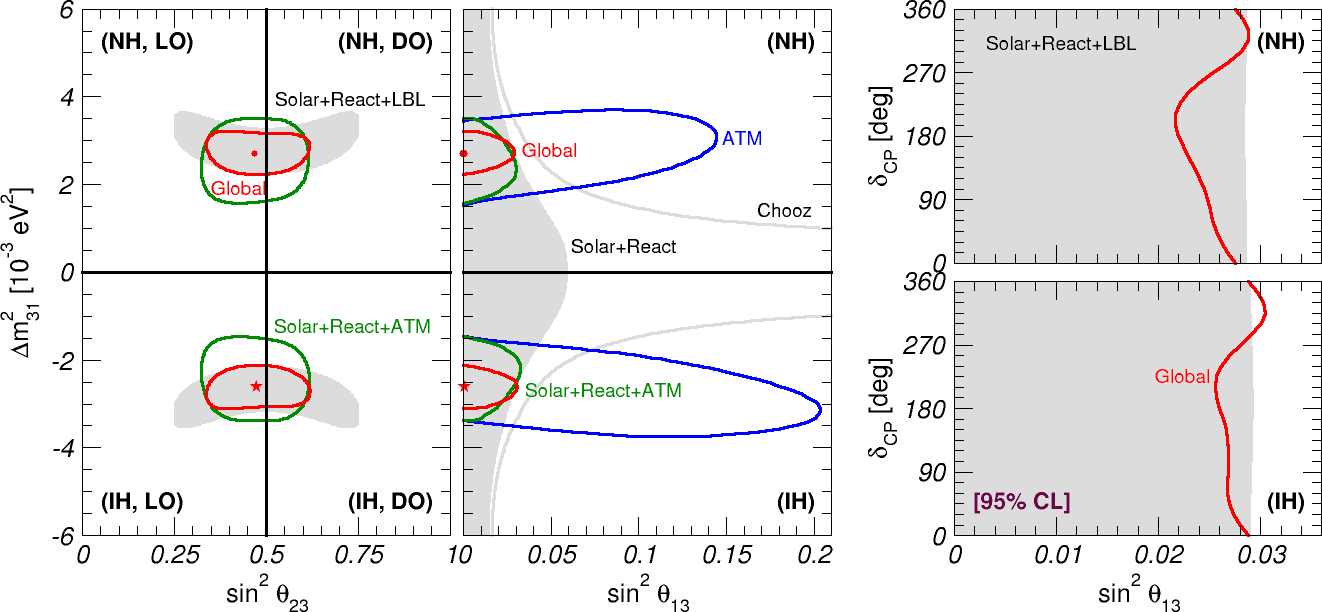
Figure 1: Allowed regions at 95% CL from the analysis of different combinations of neutrino experiments. In particular, the gray regions correspond the combination of solar, reactor and accelerator data.  

To set the basis for the following discussion, it is useful to study how much the information coming from atmospheric neutrino data contributes to this picture. The “solar” parameters $\theta_{12}$ and $\Delta m^{2}_{21}$ are completely determined by the solar and KamLAND data alone, and will therefore not be discussed here. As for the remaining parameters, in Fig. 1 we show the allowed regions implied by different combinations of neutrino experiments. It is clear from this figure that the bound on $\theta_{13}$ comes mainly from Chooz, with a small contribution from solar and KamLAND data, while the atmospheric mass-squared difference $\Delta m^{2}_{31}$ is mainly determined by the accelerator experiments K2K and Minos. The only parameter whose determination is still dominated by atmospheric data is $\theta_{23}$, being mainly a matter of total statistics. So it seems that indeed atmospheric experiments already have not much to say.

However, at a better look we note that present reactor and accelerator data (gray regions) exhibit a very high degree of symmetry. In particular, they have practically no dependence on $\delta_{\textsc{cp}}$, and they are totally insensitive to the neutrino mass hierarchy (sign of $\Delta m^{2}_{31}$) and to the octant (sign of $\theta_{23}-45^{\circ}$). Conversely, when atmospheric data are also included in the fit these ambiguities, although far from being resolved, become at least non-symmetric. In particular, the atmospheric bound on $\theta_{13}$ (blue lines) considerably depends on the mass hierarchy, and the global fit with atmospheric data included (red lines) exhibit a weak but visible dependence on the CP phase and on the octant. Of course, this is not a proof that atmospheric data will be relevant in the future, especially since the results of forthcoming accelerator experiments such as T2K will have a non-trivial dependence on the value of $\delta_{\textsc{cp}}$ and on the neutrino mass hierarchy. However, it is a hint the very broad-range information provided by atmospheric neutrino data, which span about three orders of magnitude in length and more than five in energy, may still be complementary to accelerator experiments, which despite their high degree of precision are limited to a fixed baseline and cover only a very limited range in neutrino energy. In the rest of this talk we will present a systematic study of these potentialities.

2 Sensitivity to oscillation parameters

As already mentioned, the strength of atmospheric data is its very broad interval in neutrino energy ($E_{\nu}$) and baseline (determined by the nadir angle $\Theta_{\nu}$). In order to provide a global view of this whole range, in this section we will make extensive use of neutrino oscillograms of the Earth, i.e. contours of equal probabilities in the neutrino energy–nadir angle plane. $\!{}^{{\bf?}}$ More exactly, we will show contours of equal oscillated-to-unoscillated ratio of atmospheric neutrino fluxes of flavor $\beta$ arriving at the detector, $\Phi_{\beta}/\Phi_{\beta}^{0}$, obtained by folding the primary neutrino flux $\Phi_{\alpha}^{0}$ with the relevant conversion probability $P_{\alpha\to\beta}$, so that $\Phi_{\beta}=\sum_{\alpha}\Phi_{\alpha}^{0}\,P_{\alpha\to\beta}$. As we will see, different regions of the ($E_{\nu}$, $\Theta_{\nu}$) plane will show characteristic structures whose position and size is determined by various neutrino parameters.

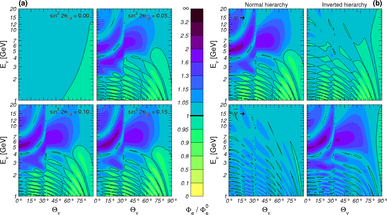
Figure 2: Oscillograms of the oscillated-to-unoscillated flux ratio $\Phi_{e}/\Phi_{e}^{0}$. Left (a): dependence on $\theta_{13}$. Right (b): dependence on the neutrino mass hierarchy.  

$\theta_{13}$. Let us start by considering the sensitivity to $\theta_{13}$. As can be seen from Fig. 2(a), for non-zero value of $\theta_{13}$ matter effects induce a resonance in the $\nu_{\mu}\to\nu_{e}$ conversion probability at $E_{\nu}\sim 3\div 6$ GeV. The precise position of this peak in the $(E_{\nu},\,\Theta_{\nu})$ plane depends on the value of $\theta_{13}$, so that in principle atmospheric neutrinos could be used to measure this angle as long as it is larger than about $3^{\circ}$. However, in practice the sensitivity is limited by two factors:

• statistics: at $E_{\nu}\sim 6$ GeV the atmospheric flux is already considerably suppressed;

• background: the $\nu_{\mu}\to\nu_{e}$ signal is diluted by the unavoidable background of $\nu_{e}\to\nu_{e}$ events.

Therefore, although some sensitivity is to be expected in a megaton detector, it is likely that atmospheric neutrinos will not be competitive with dedicated long-baseline and reactor experiments for what concerns the determination of $\theta_{13}$. However, an explicit observation of this resonance will provide a very important confirmation of the MSW and parametric-resonance mechanisms.

Hierarchy. As shown in Fig. 2(b), the sensitivity to the hierarchy arises from the observation of the same high-energy resonance which is also involved in the sensitivity to $\theta_{13}$. It is therefore only possible if $\theta_{13}$ is large enough. Note that in order to determine the hierarchy it is not sufficient to see the resonance (which would simply be a indication of non-zero $\theta_{13}$), it is also necessary to tell whether it occurred for neutrinos (normal hierarchy) or antineutrinos (inverted hierarchy). It is therefore particularly important to have a detector capable of charge discrimination. In the case of a non-magnetic detector such as a Water Cerenkov, if a resonance is observed it might still be possible to resolve the hierarchy by looking its size, since the number of neutrinos interacting in the detector is considerably larger than the number of antineutrinos and therefore a normal (inverted) hierarchy would result in a larger (smaller) signal. Note, however, that the amplitude of the peak is affected both by $\theta_{13}$ and by the value of $\theta_{23}$, as we will see in the next paragraph, so that a poorly known value of these parameters will result in a considerable loss of sensitivity.

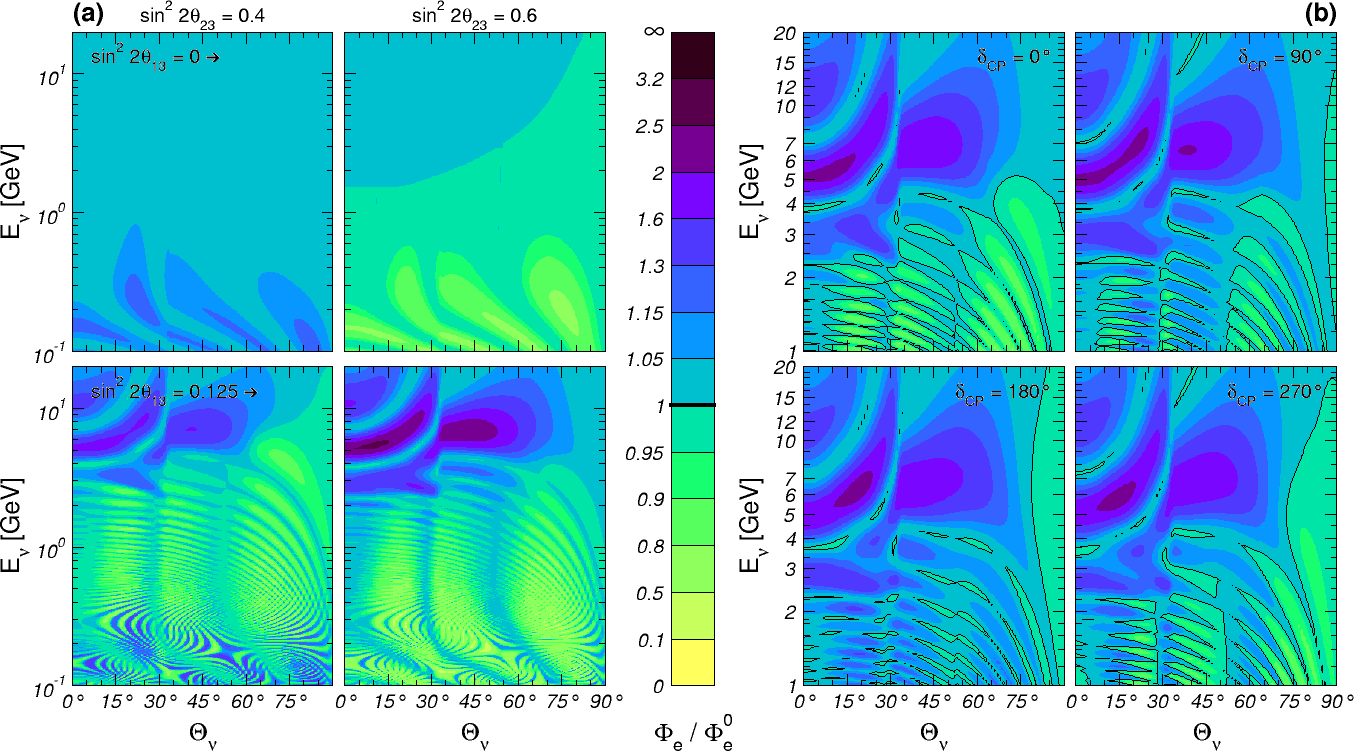
Figure 3: Oscillograms of the oscillated-to-unoscillated flux ratio $\Phi_{e}/\Phi_{e}^{0}$. Left (a): dependence on the $\theta_{23}$ octant, for $\theta_{13}=0$ and $\sin^{2}2\theta_{13}=0.125$. Right (b): dependence on the CP phase for $\sin^{2}2\theta_{13}=0.125$.  

Octant. The sensitivity to the octant is one of the topics where atmospheric neutrino are mostly useful. As can be seen Fig. 3(a), we have two characteristic signatures:

• at low energy ($E_{\nu}<1$ GeV), we observe an excess (deficit) in the $\nu_{e}$ flux with respect to maximal mixing if $\theta_{23}$ is smaller (larger) than $45^{\circ}$. This effect is due to subleading oscillations induced by $\Delta m^{2}_{21}$, and is present also for $\theta_{13}=0$. For $\theta_{13}\neq 0$ the $\nu_{e}$ flux arriving at the detector is modulated with the very fast $\Delta m^{2}_{31}$ oscillations, but the effect persists on average. Finally, this effect appears with the same sign for both neutrinos and antineutrinos, so that no charge discrimination is required for its identification.

• at high energy ($E_{\nu}>3$ GeV), we observe a decrease (increase) in the $\nu_{e}$ flux with respect to maximal mixing if $\theta_{23}$ is smaller (larger) than $45^{\circ}$. This effect is again related to the matter resonance discussed for $\theta_{13}$ and the hierarchy, and indeed it appears only for $\theta_{13}\neq 0$. As already seen, in a detector without charge discrimination the signal could be considerably suppressed.

Note that the presence of a low-energy effect independent of $\theta_{13}$ guarantees a minimum sensitivity to the octant from atmospheric neutrinos, provided that the deviation of $\theta_{23}$ from maximal mixing is large enough. This is a unique feature which will prove very synergic with long-baseline data, as we will show in the next section. Note also that the slight preference for $\theta_{23}<45^{\circ}$ visible in Fig. 1 arises precisely from this effect, and from the observation of a small excess in sub-GeV $e$-like events in Super-Kamiokande data.

CP phase. Finally, let us spend a word on the sensitivity to the CP phase. A characteristic signal is visible in the intermediate-energy region, $1~{}\text{GeV}<E_{\nu}<3$ GeV, and arises from the interference of $\Delta m^{2}_{21}$-induced and $\Delta m^{2}_{31}$-induced oscillations. Although in principle it is observable, as Fig. 1 demonstrates with present data, this effect is quite small and probably hard to disentangle from other parameters. Moreover, its presence depends crucially on the size of $\theta_{13}$, so as for the sensitivity to the hierarchy it is not “guaranteed”. In the fits which we will discuss in the rest of this talk the impact of $\delta_{\textsc{cp}}$ on the determination of the other parameters is properly taken into account, however we will not present any systematic study of the sensitivity of atmospheric data to $\delta_{\textsc{cp}}$ itself.

3 Synergies with long-baseline experiments

So far we have discussed the potentialities of atmospheric neutrinos in general terms. Let us now consider concrete experimental setups and compare their performances. In particular, we will focus on three proposed experiments: $\!{}^{{\bf?}}$

• a Beta Beam ($\beta$B) from CERN to Fréjus (130 Km). We assume 5 years of $\nu_{e}$ from ¹⁸Ne and 5 years of $\bar{\nu}_{e}$ from ⁶He at $\gamma=100$, with an average neutrino energy $\left<E_{\nu}\right>=400$ MeV. For the detector we assume the MEMPHYS Water-Cerenkov proposal, corresponding to 3 tanks of 145 Kton each;

• a Super Beam (SPL) from CERN to Fréjus (130 Km). We assume 2 years of $\nu_{\mu}$ and 8 years of $\bar{\nu}_{\mu}$ running, with an average energy $\left<E_{\nu}\right>=300$ MeV. Again we use MEMPHYS as detector;

• the T2K phase II (T2HK) experiment, corresponding to a 4MW super beam from Tokai to Kamioka (295 Km), with 2 years of $\nu_{\mu}$ and 8 years of $\bar{\nu}_{\mu}$. The detector is the proposed Hyper-Kamiokande, rescaled to 440 Kton for a fair comparison with the $\beta$B and the SPL.

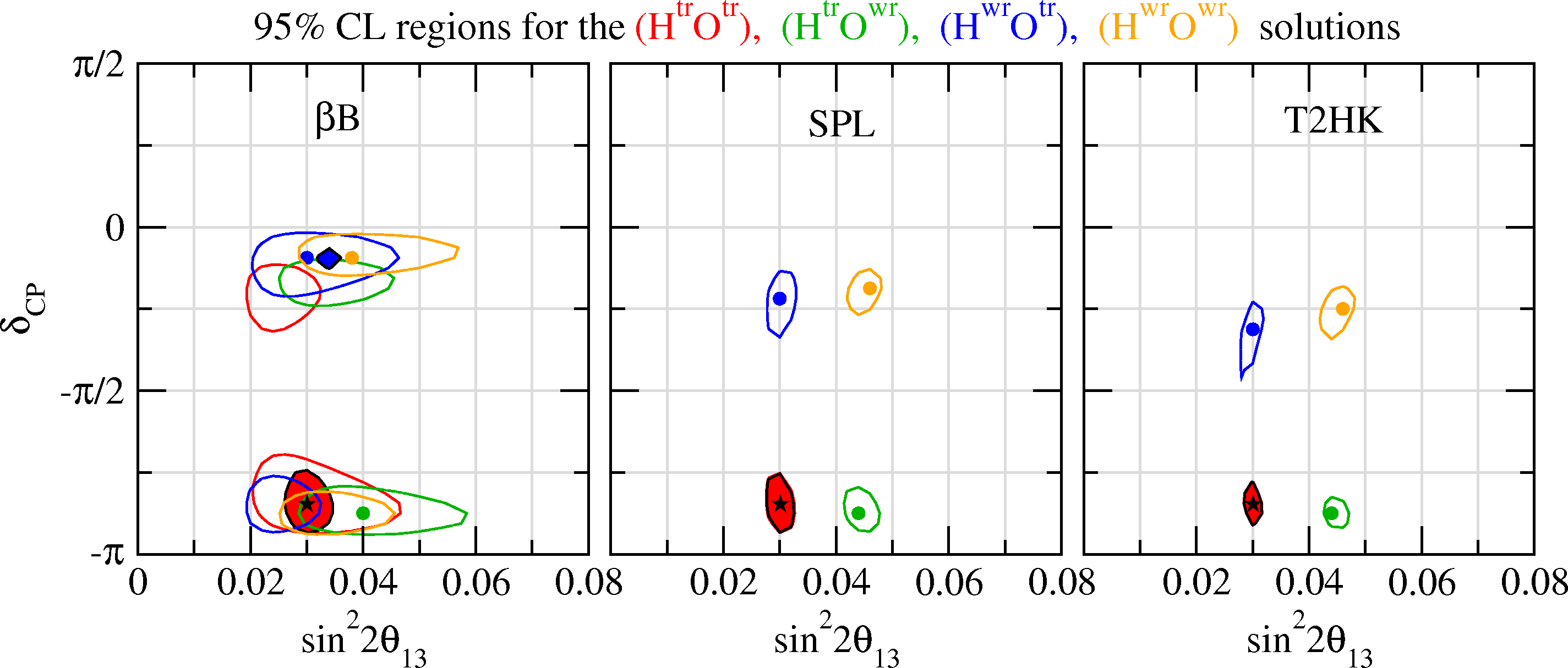
Figure 4: Allowed regions in $\sin^{2}2\theta_{13}$ and $\delta_{\mathrm{CP}}$ for LBL data alone (contour lines) and LBL+ATM data combined (colored regions). $\!{}^{{\bf?}}$ $\text{H}^{\text{tr/wr}}$ and $\text{O}^{\text{tr/wr}}$ refers to solutions with the true/wrong mass hierarchy and octant, respectively. The true parameter values are $\delta_{\textsc{cp}}=-0.85\pi$, $\sin^{2}\theta_{12}=0.3$, $\sin^{2}2\theta_{13}=0.03$, $\sin^{2}\theta_{23}=0.6$, $\Delta m^{2}_{21}=7.9\times 10^{-5}~{}\text{eV}^{2}$, $\Delta m^{2}_{31}=2.4\times 10^{-3}~{}\text{eV}^{2}$.  

A characteristic feature in the analysis of future LBL experiments is the presence of parameter degeneracies. Due to the inherent three-flavor structure of the oscillation probabilities, for a given experiment in general several disconnected regions in the multi-dimensional space of oscillation parameters will be present. Traditionally these degeneracies are referred to as follows:

• the intrinsic degeneracy: for a measurement based on the $\nu_{\mu}\to\nu_{e}$ oscillation probability for neutrinos and antineutrinos two disconnected solutions appear in the ($\delta_{\textsc{cp}},\,\theta_{13}$) plane;

• the hierarchy degeneracy: the two solutions corresponding to the two signs of $\Delta m^{2}_{31}$ appear in general at different values of $\delta_{\textsc{cp}}$ and $\theta_{13}$;

• the octant degeneracy: since LBL experiments are sensitive mainly to $\sin^{2}2\theta_{23}$ it is difficult to distinguish the two octants $\theta_{23}<45^{\circ}$ and $\theta_{23}>45^{\circ}$. Again, the solutions corresponding to $\theta_{23}$ and $\pi/2-\theta_{23}$ appear in general at different values of $\delta_{\textsc{cp}}$ and $\theta_{13}$.

This leads to an eight-fold ambiguity in $\theta_{13}$ and $\delta_{\textsc{cp}}$, and hence degeneracies provide a serious limitation for the determination of $\theta_{13}$, $\delta_{\textsc{cp}}$ and the sign of $\Delta m^{2}_{31}$. In Fig. 4 we illustrate this problem for the $\beta$B, SPL and T2HK experiments. Assuming the true parameter values $\delta_{\mathrm{CP}}=-0.85\pi$, $\sin^{2}2\theta_{13}=0.03$ and $\sin^{2}\theta_{23}=0.6$ we show the allowed regions in the plane of $\sin^{2}2\theta_{13}$ and $\delta_{\textsc{cp}}$ taking into account the solutions with the wrong hierarchy and the wrong octant. As visible in this figure, for the $\beta$B the intrinsic degeneracy cannot be resolved, due to the poor spectral information and the lack of precise information on $|\Delta m^{2}_{31}|$ and $\sin^{2}2\theta_{23}$ (usually provided by the $\nu_{\mu}$ disappearance), while for the super beam experiments SPL and T2HK there is only a four-fold degeneracy related to the sign of $\Delta m^{2}_{31}$ and the octant of $\theta_{23}$. On the other hand, once atmospheric data are included in the fit all the degeneracies are nearly completely resolved, and the true solution is identified at 95% CL. This clearly show the presence of a synergy between atmospheric and long-baseline data: at least for this specific example, the combination of the two sets is much more powerful than the simple sum of each individual data sample.

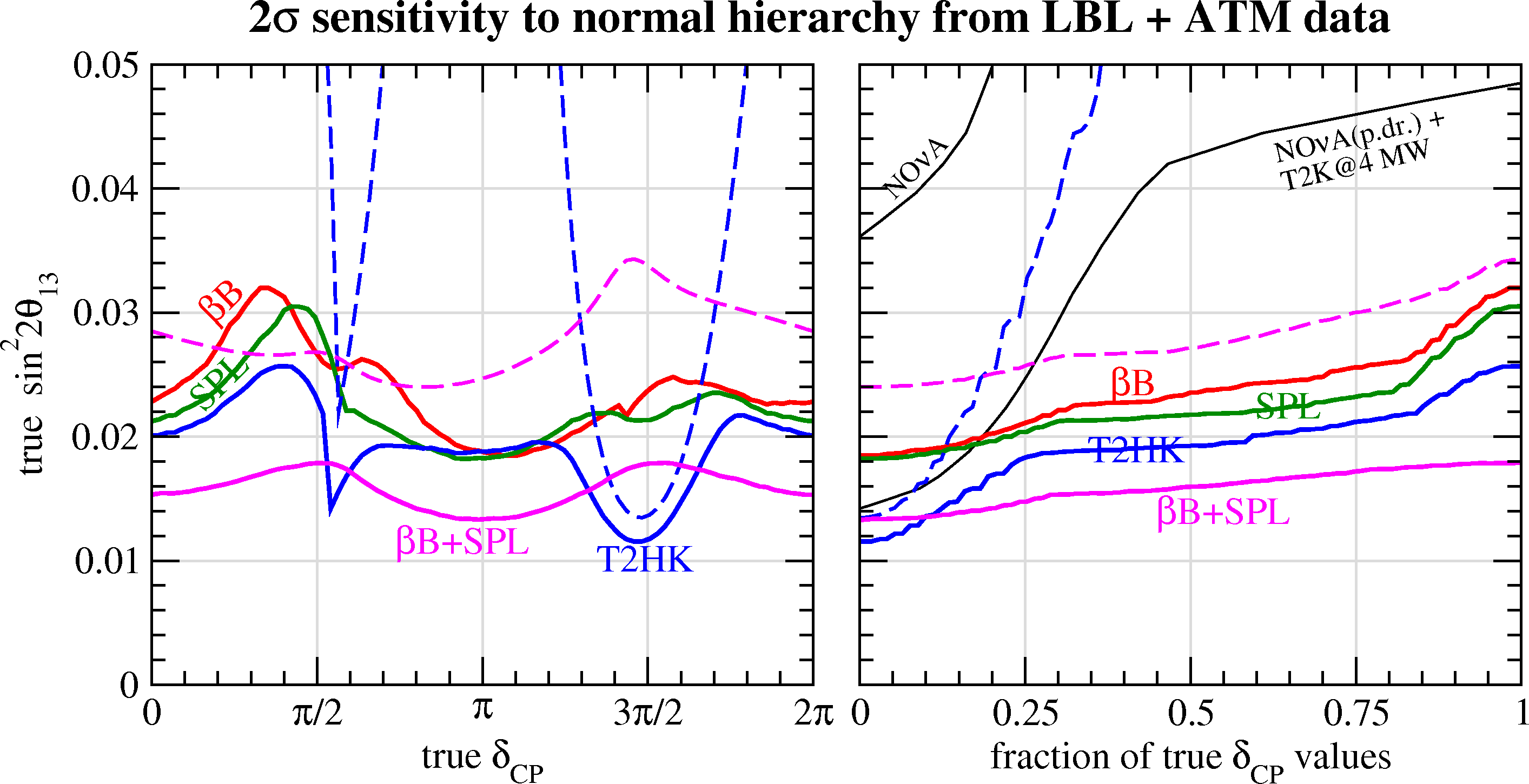
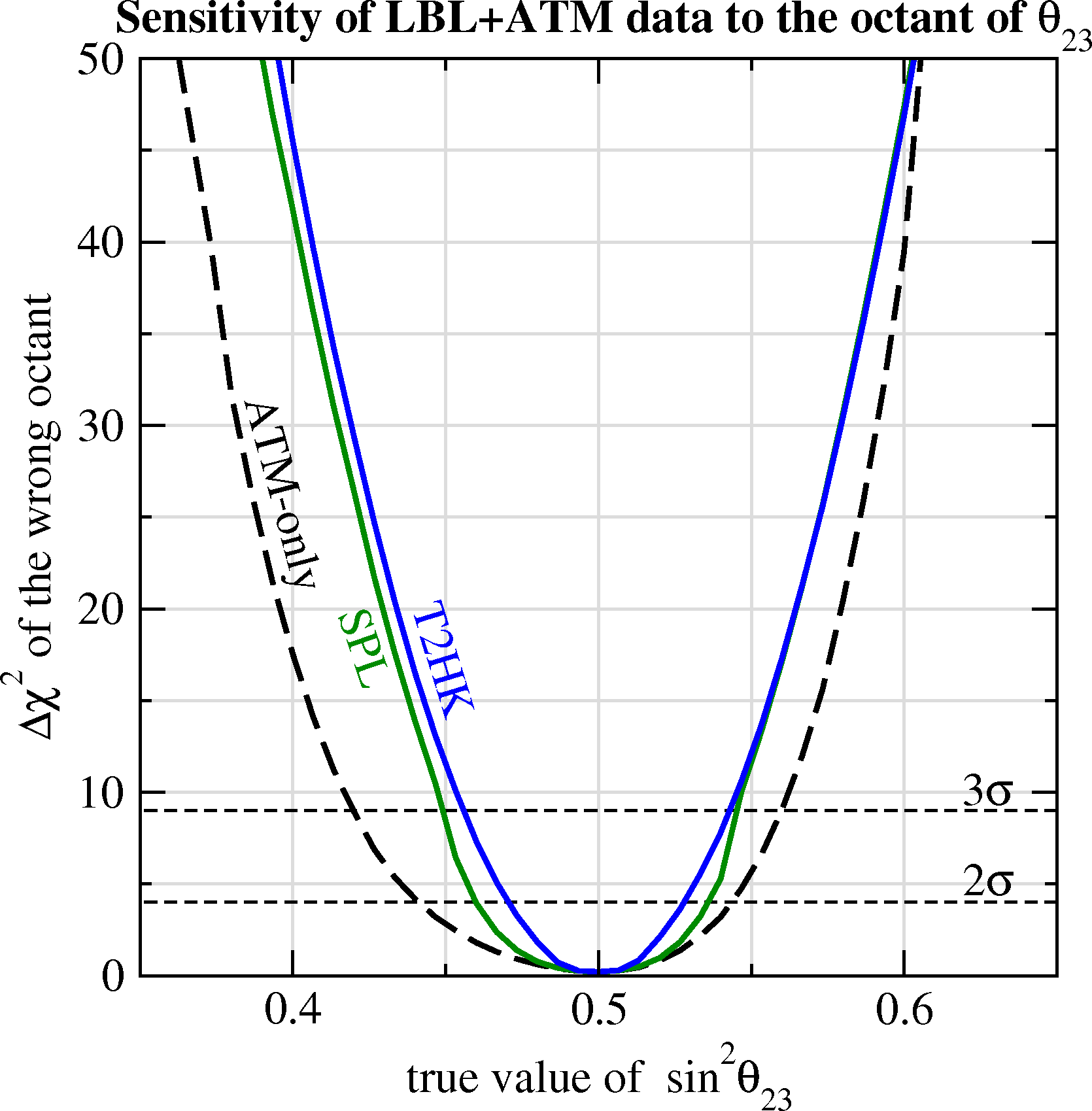
Figure 5: Left: sensitivity to the mass hierarchy at $2\sigma$ $(\Delta\chi^{2}=4)$ as a function of the true values of $\sin^{2}2\theta_{13}$ and $\delta_{\textsc{cp}}$. The solid curves are the sensitivities from the combination of long-baseline and atmospheric neutrino data, the dashed curves correspond to long-baseline data only. Right: $\Delta\chi^{2}$ of the solution with the wrong octant of $\theta_{23}$ as a function of the true value of $\sin^{2}\theta_{23}$. We have assumed a true value of $\theta_{13}=0$.  

To further investigate this synergy, in the left panels of Fig. 5 we show how the combination of ATM+LBL data leads to a non-trivial sensitivity to the neutrino mass hierarchy. For LBL data alone (dashed curves) there is practically no sensitivity for the CERN–MEMPHYS experiments (because of the very small matter effects due to the relatively short baseline), and the sensitivity of T2HK depends strongly on the true value of $\delta_{\textsc{cp}}$. However, by including the data from atmospheric neutrinos (solid curves) the mass hierarchy can be identified at $2\sigma$ CL provided $\sin^{2}2\theta_{13}\gtrsim 0.02\div 0.03$. As an example we have chosen in that figure a true value of $\theta_{23}=45^{\circ}$; in general the hierarchy sensitivity increases as $\theta_{23}$ increases. $\!{}^{{\bf?}}$ Note that the sensitivity to the neutrino mass hierarchy shown in Fig. 5 is significantly improved with respect to our previous results. $\!{}^{{\bf?}}$ There are two main reasons for this better performance: first, we use now much more bins in charged lepton energy for fully contained single-ring events; second, we implemented also the information from multi-ring events. This latter point is important since the relative contribution of neutrinos and antineutrinos is different for single-ring and multi-ring events. Therefore, combining both data sets allows to obtain a discrimination between neutrino and antineutrino events on a statistical basis. This in turn contains crucial information on the hierarchy, since as discussed in Sec. 2 the mass hierarchy determines whether the matter enhancement occurs for neutrinos or for antineutrinos.

In the right panel of Fig. 5 we show the potential of ATM+LBL data to exclude the octant degenerate solution. As seen in the previous section, this effect is based mainly on oscillations with $\Delta m^{2}_{21}$ and therefore we have very good sensitivity even for $\theta_{13}=0$; a finite value of $\theta_{13}$ in general improves the sensitivity. $\!{}^{{\bf?}}$ From the figure one can read off that atmospheric data alone can resolve the correct octant at $3\sigma$ if $|\sin^{2}\theta_{23}-0.5|\gtrsim 0.085$. If atmospheric data is combined with the LBL data from SPL or T2HK there is sensitivity to the octant for $|\sin^{2}\theta_{23}-0.5|\gtrsim 0.05$. The improvement of the octant sensitivity with respect to previous analyses $\!{}^{{\bf?},{\bf?}}$ follows from changes in the analysis of sub-GeV atmospheric events, where now three bins in lepton momentum are used instead of one. Note that since in this figure we have assumed a true value of $\theta_{13}=0$, combining the $\beta$B with ATM does not improve the sensitivity with respect to atmospheric data alone.

4 Direct determination of atmospheric fluxes

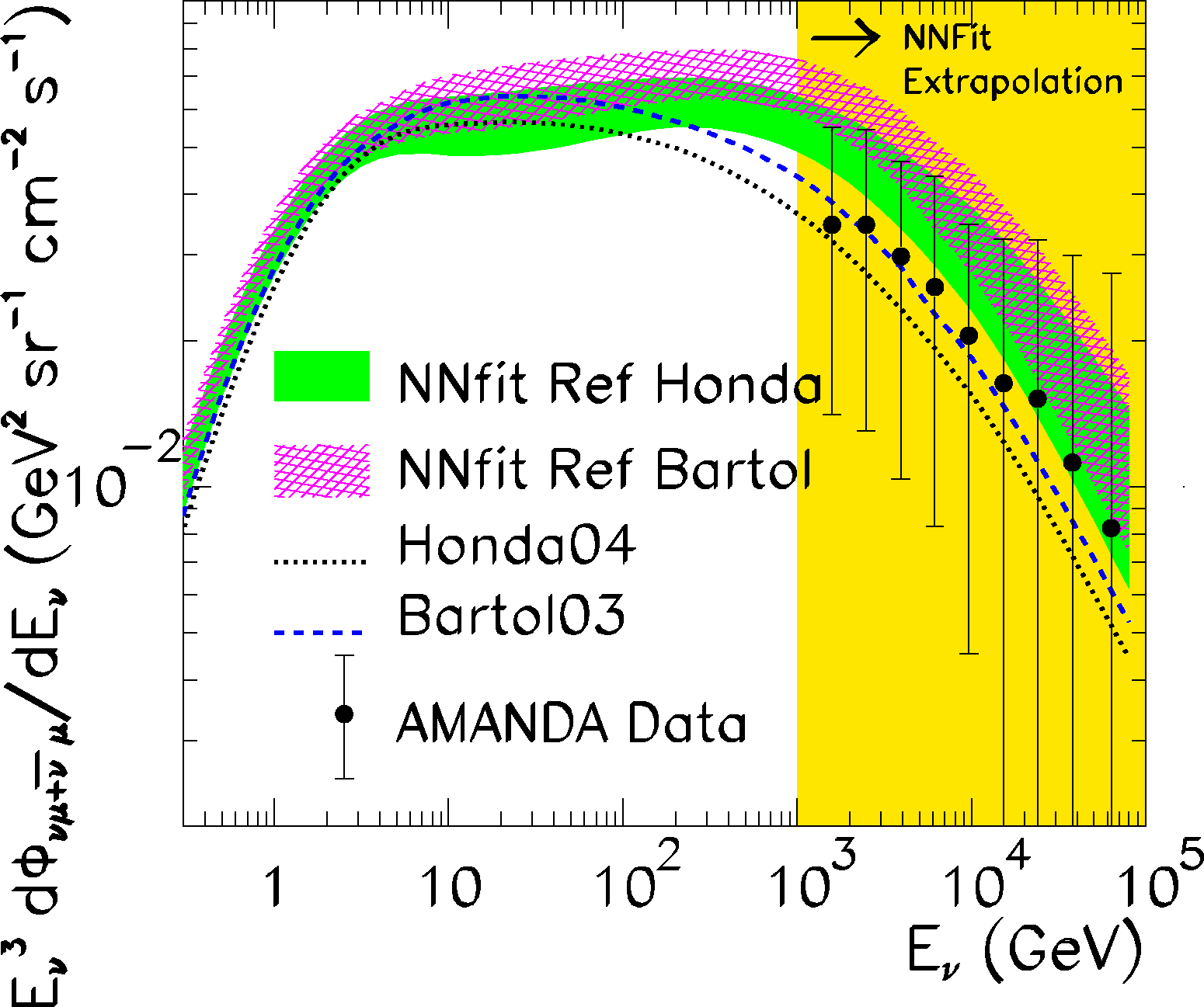
Figure 6: Results for the reference fit for the angular averaged muon neutrino plus antineutrino flux extrapolated to the high-energy region compared to the corresponding data from AMANDA. Also shown are the results with different reference fluxes and the comparison with the predictions of different flux models.  

So far we have discussed the potentialities of atmospheric neutrino for what concerns the determination of the neutrino parameters. The main message of the first part of this talk is that atmospheric data can provide very useful information on the neutrino mass matrix, despite the very large uncertainties in the neutrino fluxes. However, it is logically acceptable to invert the strategy, and to regard the poorly known atmospheric neutrino fluxes as a subject of investigation themselves. In this section we will therefore assume that the neutrino parameters have been accurately measured by other experiments, and we will show that it is possible to extract the the atmospheric neutrino fluxes directly from the data. $\!{}^{{\bf?}}$

There are several motivations for such direct determination of the atmospheric neutrino fluxes. First of all it would provide a cross-check of the standard flux calculations as well as of the size of the associated uncertainties (which, being mostly theoretical, are difficult to quantify). Second, a precise knowledge of the atmospheric neutrino flux is of importance for high energy neutrino telescopes, both because they are the main background and they are used for detector calibration. Finally, such program may quantitatively expand the physics potential of future atmospheric neutrino experiments. Technically, however, this program is challenged by the absence of a generic parametrization of the energy and angular functional dependence of the fluxes which is valid in all the range of energies where there is available data. We bypass this problem by using artificial neural networks as unbiased interpolants for the unknown neutrino fluxes. However, the precision of the available experimental data is not yet enough to allow for a separate determination of the energy, zenith angle and flavor dependence of the atmospheric flux. Consequently in our work we have assumed the zenith and flavor dependence of the flux to be known with some precision and extract from the data only its energy dependence. Thus the neural network flux parametrization will be:

$$\Phi^{\text{fit}}_{\alpha,\pm}(E_{\nu},c_{a},h)=F^{\text{fit}}(E_{\nu})\,\Phi^{\text{ref}}_{\alpha,\pm}(E_{\nu},c_{a},h)$$ (4)

where $F^{\text{fit}}(E_{\nu})$ is the neural network output when the input is the neutrino energy $E_{\nu}$.

In Fig. 6 we show the results of our fit to the atmospheric neutrino flux as compared with the computations of the Honda $\!{}^{{\bf?}}$ and Bartol $\!{}^{{\bf?}}$ groups. The results of the neural network fit are shown in the form of a $1\sigma$ band, and plotted as a function of the neutrino energy. For comparison we also show the data from AMANDA. $\!{}^{{\bf?}}$ We see from this figure that the flux obtained from the fit is in reasonable agreement with the theoretical calculations, although the fit seems to prefer a slightly higher flux at higher energies. This indicates that until about $E_{\nu}\sim 1$ TeV we have a good understanding of the normalization of the fluxes, and that the present accuracy from Super-Kamiokande neutrino data is comparable with the theoretical uncertainties from the numerical calculations. Note also that the results of our alternative fits depends only mildly on the choice of Honda or Bartol as the reference flux. This suggests that the present uncertainties on the angular dependence have been properly estimated, so that the assumed angular dependence has very little effect on the determination of the energy dependence of the fluxes. Thus the atmospheric neutrino flux determined with our method could be used as an alternative to the existing flux calculations.

5 Conclusions

In this talk we have discussed the potentialities of atmospheric neutrino data in the context of future neutrino experiments. We have shown that despite the large uncertainties in the neutrino fluxes atmospheric data will still provide useful information on the neutrino parameters, due to their very broad range in neutrino energy and nadir angle. In particular, we have proved that the sensitivity obtained by a combination of atmospheric and long-baseline data is much stronger than the one achievable by each data set separately. Finally, we have shown that present atmospheric data can be used to obtain a direct determination of the atmospheric neutrino fluxes.

References

- [1] M. C. Gonzalez-Garcia and M. Maltoni, arXiv:0704.1800 [hep-ph].
- [2] E. Kh. Akhmedov et al., JHEP 05 (2007) 077 [arXiv:hep-ph/0612285].
- [3] J. E. Campagne et al., JHEP 04 (2007) 003 [arXiv:hep-ph/0603172].
- [4] P. Huber et al., Phys. Rev. D 71 (2005) 053006 [arXiv:hep-ph/0501037].
- [5] M. C. Gonzalez-Garcia et al., Phys. Rev. D 70 (2004) 093005 [arXiv:hep-ph/0408170].
- [6] M. C. Gonzalez-Garcia et al., JHEP 10 (2006) 075 [arXiv:hep-ph/0607324].
- [7] M. Honda et al., Phys. Rev. D 70 (2004) 043008 [arXiv:astro-ph/0404457].
- [8] G. D. Barr et al., Phys. Rev. D 70 (2004) 023006 [arXiv:astro-ph/0403630].
- [9] A. Achterberg et al. [IceCube Collaboration], arXiv:astro-ph/0509330.