Transversity and Collins Functions:
from $e^{+}e^{-}\to h_{1}h_{2}X$ to SIDIS Processes

Abstract

We present [1] the first simultaneous extraction of the transversity distribution and the Collins fragmentation function, obtained through a combined analysis of experimental data on azimuthal asymmetries in semi-inclusive deep inelastic scattering (SIDIS), from the HERMES and COMPASS Collaborations, and in $e^{+}e^{-}\to h_{1}h_{2}X$ processes, from the Belle Collaboration.

Among the three leading twist parton distributions, that contain basic information on the internal structure of nucleons, the transversity distribution is the most difficult to access. Due to its chiral-odd nature it can only appear in physical processes which require a quark helicity flip. At present the most accessible channel is the SIDIS process with a polarized target, where the corresponding azimuthal asymmetry, $A_{UT}^{\sin(\phi_{S}+\phi_{h})}$, involves the transversity distribution coupled to the Collins fragmentation function [2], also unknown. Indeed it has received a lot of attention in the ongoing experimental programs of HERMES [3], COMPASS [4], and JLab Collaborations.

A crucial breakthrough in this strategy has recently been achieved with the independent measurement of the Collins function via the azimuthal correlation observed in the two-pion production in $e^{+}e^{-}$ annihilation by the Belle Collaboration at KEK [5].

Let us start with the $e^{+}e^{-}\to h_{1}h_{2}X$ process. We choose the reference frame so that the elementary $e^{+}e^{-}\to q\bar{q}$ scattering occurs in the $\hat{xz}$ plane, with the back-to-back quark and antiquark moving along the $\hat{z}$-axis identified as the jet thrust axis. The cross section corresponding to this process can be expressed as (see Ref. [6]):

$$\frac{d\sigma^{e^{+}e^{-}\to h_{1}h_{2}X}}{dz_{1}\,dz_{2}\,d^{2}{\mbox{\boldmath$p$}}_{\perp 1}\,d^{2}{\mbox{\boldmath$p$}}_{\perp 2}\,d\cos\theta} = \frac{3\pi\alpha^{2}}{2s}\,\sum_{q}e_{q}^{2}\,\Big{\{}(1+\cos^{2}\theta)\,D_{h_{1}/q}(z_{1},p_{\perp 1})\,D_{h_{2}/\bar{q}}(z_{2},p_{\perp 2})\Big{.}$$

$$+\,\Big{.}\frac{1}{4}\,\sin^{2}\theta \Delta^{N}D_{h_{1}/q^{\uparrow}}(z_{1},p_{\perp 1})\,\Delta^{N}D_{h_{2}/\bar{q}^{\uparrow}}(z_{2},p_{\perp 2})\,\cos(\varphi_{1}+\varphi_{2})\Big{\}}\,,$$ (1)

where $\varphi_{i}$ are the azimuthal angles identifying the direction of the observed hadron $h_{i}$ in the helicity frame of the fragmenting quark $q$, $z_{i}$ and $\mbox{\boldmath$p$}_{\perp i}$ are the hadron light-cone momentum fractions and transverse momenta, and $\theta$ is the scattering angle in the $e^{+}e^{-}\to q\bar{q}$ process. $\Delta^{N}D_{h/q^{\uparrow}}(z,p_{\perp})$ is the Collins function, also known as $H_{1}^{\perp}$ (see Ref. [7]). To compare with data we have to $i)$ perform a change of angular variables from $(\varphi_{1},\varphi_{2})$ to $(\varphi_{1},\varphi_{1}+\varphi_{2})$ and integrate over $p_{\perp 1}$, $p_{\perp 2}$, and over $\varphi_{1}$; $ii)$ normalize the result to the azimuthal averaged cross section; $iii)$ take the ratio $R$ of unlike-sign to like-sign pion-pair production:

$$R\simeq 1+\cos(\varphi_{1}+\varphi_{2})\,A_{12}(z_{1},z_{2})\>,\quad{\rm where}\quad A_{12}(z_{1},z_{2})=\frac{1}{4}\,\frac{\langle\sin^{2}\theta\rangle}{\langle 1+\cos^{2}\theta\rangle}\,(P_{U}-P_{L})\>,$$ (2)

the angle $\theta$ is averaged over a range of values given by the detector acceptance,

$$P_{U(L)}=\frac{\sum_{q}e^{2}_{q}\,\Delta^{N}D_{\pi^{+}/q^{\uparrow}}(z_{1})\,\Delta^{N}D_{\pi^{-(+)}/\bar{q}^{\uparrow}}(z_{2})}{\sum_{q}e^{2}_{q}D_{\pi^{+}/q}(z_{1})\,D_{\pi^{-(+)}/\bar{q}}(z_{2})}\>,\quad{\rm and}$$ (3)

$$\Delta^{N}D_{h/q^{\uparrow}}(z)=\int d^{2}\mbox{\boldmath$p$}_{\perp}\Delta^{N}D_{h/q^{\uparrow}}(z,p_{\perp})=\int d^{2}\mbox{\boldmath$p$}_{\perp}\frac{2p_{\perp}}{zm_{h}}\;H_{1}^{\perp q}(z,p_{\perp})=4\;H_{1}^{\perp(1/2)q}(z)\>.$$ (4)

For fitting purposes, it is convenient to re-express $P_{U}$ and $P_{L}$ in terms of favoured and unfavoured fragmentation functions (and similarly for the $\Delta^{N}D$),

$$D_{\pi^{+}/u,\bar{d}}=D_{\pi^{-}/d,\bar{u}}\equiv D_{\rm fav}\,;\;\;\;D_{\pi^{+}/d,\bar{u}}=D_{\pi^{-}/u,\bar{d}}=D_{\pi^{\pm}/s,\bar{s}}\equiv D_{\rm unf}\,.$$ (5)

In addition, the Belle Collaboration presents the same set of data, analysed in a different reference frame: following Ref. [7], one can fix the $\hat{z}$-axis as given by the direction of the observed hadron $h_{2}$ and the $\hat{xz}$ plane as determined by the lepton and the $h_{2}$ directions. An azimuthal dependence of the other hadron $h_{1}$ with respect to this plane has been measured. In this configuration the corresponding ratio becomes

$$R\simeq 1+\cos(2\,\phi_{1})A_{0}(z_{1},z_{2})\,,\;\;\;\;A_{0}(z_{1},z_{2})=\frac{1}{\pi}\,\frac{z_{1}\,z_{2}}{z_{1}^{2}+z_{2}^{2}}\,\frac{\langle\sin^{2}\theta_{2}\rangle}{\langle 1+\cos^{2}\theta_{2}\rangle}\,(P_{U}-P_{L})\,.$$ (6)

Let us now consider the SIDIS process $\ell\,p\to\ell\,h\,X$. We take, in the $\gamma^{*}-p$ c.m. frame, the virtual photon and the proton colliding along the $\hat{z}$-axis with momenta $q$ and $P$ respectively, and the leptonic plane to coincide with the $\hat{xz}$ plane.

To single out the spin dependent part of the fragmentation of a transversely polarized quark we consider the $\sin(\phi_{S}+\phi_{h})$ weighted asymmetry (at ${\cal O}(k_{\perp}/Q)$):

$$A^{\sin(\phi_{S}+\phi_{h})}_{{UT}}=2\,\frac{\int d\phi_{S}\,d\phi_{h}\,[d\sigma^{\uparrow}-d\sigma^{\downarrow}]\,\sin(\phi_{S}+\phi_{h})}{\int d\phi_{S}\,d\phi_{h}\,[d\sigma^{\uparrow}+d\sigma^{\downarrow}]}$$ (7)

$$=\frac{\displaystyle\sum_{q}e_{q}^{2}\!\!\int\!\!{d\phi_{S}d\phi_{h}d^{2}\mbox{\boldmath$k$}_{\perp}}\Delta_{T}q(x,k_{\perp})\!\frac{d(\Delta{\hat{\sigma}})}{dy}\Delta^{N}\!D_{h/q^{\uparrow}}(z,p_{\perp})\sin(\phi_{S}+\varphi+\phi_{q}^{h})\sin(\phi_{S}+\phi_{h})}{\displaystyle\sum_{q}e_{q}^{2}\int{d\phi_{S}d\phi_{h}\,d^{2}\mbox{\boldmath$k$}_{\perp}}f_{q/p}(x,k_{\perp})\frac{d\hat{\sigma}}{dy}D_{h/q}(z,p_{\perp})}\,\cdot$$

In the above equation $\Delta_{T}q(x,k_{\perp})$ is the unintegrated transversity distribution, $d{\hat{\sigma}}/dy$ is the planar unpolarized elementary cross section and $\frac{d(\Delta{\hat{\sigma}})}{dy}=\frac{4\pi\alpha^{2}}{sxy^{2}}\,(1-y)$. The $\sin(\phi_{S}+\varphi+\phi_{q}^{h})$ azimuthal dependence in Eq. (7) arises from the combination of the phase factors in the transversity distribution function, in the non-planar $\ell\,q\to\ell\,q$ elementary scattering amplitudes, and in the Collins fragmentation function (see Ref. [6] and [8]). We assume

$$f_{q/p}(x,k_{\perp})=f_{q/p}(x)\;\frac{e^{-{k_{\perp}^{2}}/\langle k_{\perp}^{2}\rangle}}{\pi\langle k_{\perp}^{2}\rangle}\;,\hskip 14.22636ptD_{h/q}(z,p_{\perp})=D_{h/q}(z)\;\frac{e^{-p_{\perp}^{2}/\langle p_{\perp}^{2}\rangle}}{\pi\langle p_{\perp}^{2}\rangle}\;,$$ (8)

where $f_{q/p}(x)$ and $D_{h/q}(z)$ are the usual integrated parton distribution and fragmentation functions and the average values of $k_{\perp}^{2}$ and $p_{\perp}^{2}$ are taken from Ref. [9]: $\langle k_{\perp}^{2}\rangle=0.25\>\textrm{GeV}^{2}$, $\langle p_{\perp}^{2}\rangle=0.20\>\textrm{GeV}^{2}$. For the transversity and the Collins functions we choose

$$\Delta_{T}q(x,k_{\perp})=\frac{1}{2}\,{\cal N}^{T}_{q}(x)\,\left[f_{q/p}(x)+\Delta q(x)\right]\;\frac{e^{-{k_{\perp}^{2}}/{\langle k_{\perp}^{2}\rangle}}}{\pi\langle k_{\perp}^{2}\rangle}\,,$$ (9)

$$\Delta^{N}D_{h/q^{\uparrow}}(z,p_{\perp})=2\,{\cal N}^{C}_{q}(z)\;D_{h/q}(z,p_{\perp})\,\sqrt{2e}\,\frac{p_{\perp}}{M}\,e^{-{p_{\perp}^{2}}/{M^{2}}}\,,$$ (10)

$${\cal N}^{T}_{q}(x)=N^{T}_{q}\,x^{\alpha}(1-x)^{\beta}\,\frac{(\alpha+\beta)^{(\alpha+\beta)}}{\alpha^{\alpha}\beta^{\beta}}\,,\;\;{\cal N}^{C}_{q}(z)=N^{C}_{q}\,z^{\gamma}(1-z)^{\delta}\,\frac{(\gamma+\delta)^{(\gamma+\delta)}}{\gamma^{\gamma}\delta^{\delta}}\,,$$ (11)

with $|N^{T}_{q}|,\>|N^{C}_{q}|\leq 1$ and where $\Delta q$ is the helicity distribution.

Notice that our parameterizations are devised in such a way that the transversity distribution function and the Collins function automatically obey their proper bounds.

By insertion of the above expressions into Eq. (7), we obtain

$$A^{\sin(\phi_{S}+\phi_{h})}_{{UT}}=\frac{\displaystyle\frac{P_{T}}{M}\frac{1-y}{sxy^{2}}\sqrt{2e}\frac{\langle p_{\perp}^{2}\rangle^{2}_{{}_{C}}}{\langle p_{\perp}^{2}\rangle}\frac{e^{-P_{T}^{2}/\langle P_{T}^{2}\rangle_{{}_{C}}}}{\langle P_{T}^{2}\rangle^{2}_{{}_{C}}}\sum_{q}e_{q}^{2}{\cal N}^{{}_{{}_{T}}}_{q}(x)\left[f_{q/p}(x)+\Delta q(x)\right]{\cal N}^{{}_{{}_{C}}}_{q}(z)D_{h/q}(z)}{\displaystyle\frac{e^{-P_{T}^{2}/\langle P_{T}^{2}\rangle}}{\langle P_{T}^{2}\rangle}\frac{[1+(1-y)^{2}]}{sxy^{2}}\,\sum_{q}e_{q}^{2}\,f_{q/p}(x)\;D_{h/q}(z)}\;,$$ (12)

$${\rm with}\;\,\langle p_{\perp}^{2}\rangle_{{}_{C}}=\frac{M^{2}\langle p_{\perp}^{2}\rangle}{M^{2}+\langle p_{\perp}^{2}\rangle}\,,\quad\quad\langle P_{T}^{2}\rangle=\langle p_{\perp}^{2}\rangle+z^{2}\langle k_{\perp}^{2}\rangle\,,\quad\quad\langle P_{T}^{2}\rangle_{{}_{C}}=\langle p_{\perp}^{2}\rangle_{{}_{C}}+z^{2}\langle k_{\perp}^{2}\rangle\,.$$ (13)

Using the above expressions for $\Delta_{T}q$ and $\Delta^{N}D_{\pi/q^{\uparrow}}$ both in $A^{\sin(\phi_{S}+\phi_{h})}_{{UT}}$, Eq. (12), and in $A_{12}$, Eq. (2), we can fix all free parameters by performing a best fit of the HERMES, COMPASS and Belle data. We checked that using $A_{0}$ instead of $A_{12}$ leads to a consistent extraction (see Ref. [6] for details).

Our results are collected in Figs. 1, 2 where we present a comparison of our curves with the data. Figure 3 shows our extracted transversity distributions and Collins functions.

Summarizing, our global analysis of present data on azimuthal asymmetries measured in SIDIS and $e^{+}e^{-}\to\pi\pi X$ allows to get quantitative estimates of both the transversity and the Collins function. In particular, we find: $i)$ $|\Delta_{T}u|>|\Delta_{T}d|$, and both smaller than the corresponding Soffer bound; $ii)$ $\Delta_{T}u$ tightly constrained by HERMES data alone, whereas COMPASS data help in constraining the transversity for $d$ quarks; $iii)$ unfavoured Collins functions larger in size (and opposite in sign) than the favoured ones.

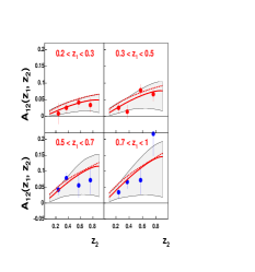
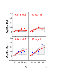
Figure 1: Data on two different azimuthal correlations in unpolarized $e^{+}e^{-}\to h_{1}h_{2}\,X$ processes, as measured by Belle Collaboration [5], compared to the curves obtained from our fit. The solid (dashed) lines correspond to the global fit obtained including the $A_{12}$($A_{0}$) asymmetry; the shaded area corresponds to the theoretical uncertainty on the parameters.

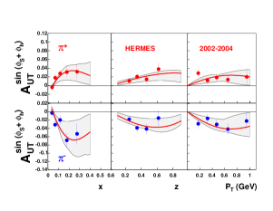
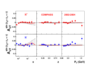
Figure 2: Our results compared with HERMES data [3] on $A_{{UT}}^{\sin(\phi_{S}+\phi_{h})}$ for $\pi^{\pm}$ production (left panel) and COMPASS data on $A_{{UT}}^{\sin(\phi_{S}+\phi_{h})}$, for the production of positively and negatively charged hadrons off a deuterium target [4] (right panel).

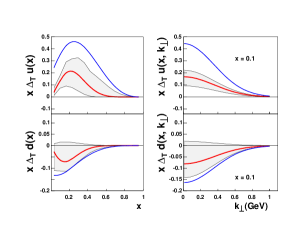
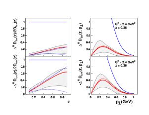
Figure 3: First panel: $x\,\Delta_{T}u(x)$ (upper plot) and $x\,\Delta_{T}d(x)$ (lower plot), vs. $x$ at $Q^{2}=2.4$ GeV². The Soffer bound is also shown for comparison (bold blue line). Second panel: $x\,\Delta_{T}u(x,k_{\perp})$ (upper plot) and $x\,\Delta_{T}d(x,k_{\perp})$ (lower plot), vs. $k_{\perp}$ at a fixed value of $x$. Third panel: the $z$ dependence of the moment of the Collins functions, Eq. (4), normalized to twice the unpolarized fragmentation functions; also shown the results of Refs. [10] (dashed line) and [11] (dotted line). Fourth panel: the $p_{\perp}$ dependence of the Collins functions.