Perturbative QCD analysis of exclusive $J/\psi+\eta_{c}$ production in $e^{+}e^{-}$ annihilation

Abstract

We analyze the exclusive charmonium $J/\psi+\eta_{c}$ pair production in $e^{+}e^{-}$ annihilation using the nonfactorized perturbative QCD and the light-front quark model(LFQM) that goes beyond the peaking approximation. We effectively include all orders of higher twist terms in the leading order of QCD coupling constant and compare our nonfactorized analysis with the usual factorized analysis in the calculation of the cross section. We also calculate the quark distribution amplitudes, the Gegenbauer moments, and the decay constants for $J/\psi$ and $\eta_{c}$ mesons using our LFQM. Our nonfactorized result enhances the NRQCD result by a factor of $3\sim 4$ at $\sqrt{s}=10.6$ GeV.

I Introduction

It has been known that the exclusive pair production of heavy meson can be reliably predicted within the framework of perturbative quantum chromodynamics(PQCD), since the wave function is well constrained by the nonrelativistic consideration BJ85 . However, the large discrepancy between the theoretical predictions BJ03 ; LHC03 ; HKQ03 ; Kis based on the nonrelativistic QCD(NRQCD) VS factorization approach and the experimental results Belle ; Babar for the exclusive $J/\psi+\eta_{c}$ production in $e^{+}e^{-}$ annihilation at the energy $\sqrt{s}=10.6$ GeV has triggered the need of better understanding both in the available calculational tools and the appreciable relativistic effects.

A particularly convenient and intuitive framework in applying PQCD to exclusive processes is based upon the light-front(LF) Fock-state decomposition of hadronic state. If the PQCD factorization theorem is applicable, then the invariant amplitude for exclusive processes factorizes into the convolution of the valence quark distribution amplitudes(DAs) $\phi(x,q^{2})$ with the hard scattering amplitude $T_{H}$, which is dominated by one-gluon exchange diagrams at leading order of QCD coupling constant $\alpha_{s}$. To implement the factorization theorem at high momentum transfer, the hadronic wave function plays an important role linking between the long distance nonperturbative QCD and the short distance PQCD. In the LF framework, the valence quark DA is computed from the valence LF wave function $\Psi_{n}(x_{i},{\bf k}_{\perp i})$ of the hadron at equal LF time $\tau=t+z/c$ which is the probability amplitude to find $n$ constituents(quarks,antiquarks, and gluons) with LF momenta $k_{i}=(x_{i},{\bf k}_{\perp i})$ in a hadron. Here, $x_{i}$ and ${\bf k}_{\perp i}$ are the LF longitudinal momentum fraction and the transverse momenta of the $i$th constituent in the $n$-particle Fock-state, respectively.

The NRQCD factorization approach BJ03 ; LHC03 ; HKQ03 ; Kis for charmonium production assumes that the constituents are sufficiently nonrelativistic so that the relative motion of valence quarks can be neglected inside the meson. In this case, the quark DA becomes the $\delta$ function, i.e. $\phi(x,q^{2})\sim\delta(x-1/2)$(the so-called peaking approximation). However, the cross section value BJ03 ; LHC03 ; HKQ03 ; Kis estimated within the NRQCD factorization approach in the leading order of $\alpha_{s}$ underestimates the experimental data Belle ; Babar by an order of magnitude. In order to reduce the discrepancy between theory and experiment, the authors in Refs. BC ; Ma ; BLL05 ; Huang considered a rather broad quark DA instead of $\delta$-shaped quark DA.

However, as pointed out in Refs. JP ; CJD , if the quark DA is not an exact $\delta$ function, i.e. ${\bf k}_{\perp}$ in the soft bound state LF wave function can play a significant role, the factorization theorem is no longer applicable. To go beyond the peaking approximation, the invariant amplitude should be expressed in terms of the LF wave function $\Psi(x_{i},{\bf k}_{\perp i})$ rather than the quark DA. In Refs. JP ; CJD , we discussed the validity issue of peaking approximation for the heavy pseudoscalar meson pair production processes such as $e^{+}e^{-}\to P+P$($P=B_{c},B_{s},B,D,D_{s}$) using the LF model wave function $\Psi(x_{i},{\bf k}_{\perp i})\propto\exp(-M^{2}_{0}/\beta^{2})$, where $M_{0}$ is the invariant mass of the constituent quark and antiquark defined by $M^{2}_{0}=\sum_{i}({\bf k}^{2}_{\perp}+m^{2}_{i})/x_{i}$ and $\beta$ is the gaussian parameter. The gaussian parameter $\beta$ in our model wave function was found to be related to the transverse momentum via $\beta=\sqrt{\langle{\bf k}^{2}_{\perp}\rangle}$. This relation naturally explains the zero-binding energy limit as the zero transverse momentum, i.e. $\langle M^{2}_{0}\rangle=(m_{1}+m_{2})^{2}$ and $x_{i}=m_{i}/M$ for $\beta=0$. We also found that the heavy quark DA is sensitive to the value of $\beta$ and indeed quite different from the $\delta$-type DA according to our LFQM based on the variational principle for the QCD-motivated Hamiltonian CJ1 ; CJ2 . In going beyond the peaking approximation, we stressed a consistency of the formulation by keeping the transverse momentum ${\bf k}_{\perp}$ both in the wave function part and the hard scattering part together before doing any integration in the amplitude. Similar consideration has also been made in the recent investigation of the relativistic and bound state effectsEM not based on the light-front dynamics(LFD) but including the relativistic effects up to the second order of the relative quark velocity, i.e. $\langle v^{2}\rangle$. Such non-factorized analysis should be distinguished from the factorized analysis BC ; Ma ; BLL05 where the transverse momenta are seperately integrated out in the wave function part and in the hard scattering part. Even if the used LF wave functions lead to the similar shapes of DAs, it is apparent that the predictions for the cross sections of heavy meson productions would be different between the factorized and non-factorized analyses.

In this work, we extend our previous works JP ; CJD of pseudoscalar meson pair production to the case of pseudoscalar and vector meson productions and calculate the cross section for $e^{+}e^{-}\to J/\psi+\eta_{c}$ process at leading order of $\alpha_{s}$ including effectively all orders of higher twist terms. As noted in CJD , our results for the quark DA of $J/\psi$ and $\eta_{c}$ are quite different from the $\delta$-type function. We find that the non-factorized form of the form factor enhances the cross section of NRQCD result by a factor of $3\sim 4$ at $\sqrt{s}=10.6$ GeV while it reduces that of the factorized formulation by 20$\%$. Since the cross section for $e^{+}e^{-}\to J/\psi+\eta_{c}$ is found to be very sensitive to the behavior of the end points ($x\to 0$ and 1) in the quark DA, we also examine the results of the decay constants or equivalently the Gegenbauer moments of $J/\psi$ and $\eta_{c}$ mesons. Since the perturbative corrections of order $\alpha_{s}$ to the production amplitude has already been obtainedZGC increasing the cross section significantly, it is important to consider the more accurate assessment of cross section at the leading order of $\alpha_{s}$.

The paper is organized as follows. In Sec. II, we describe the formulation of our light-front quark model (LFQM), which has been quite successful in describing the static and non-static properties of the pseudoscalar and vector mesons CJ1 ; CJ2 . The formulae for the quark DA, decay constants, Gegenbauer and $\xi(=x_{1}-x_{2})$ moments are also given in this section. In Sec. III, the transverse momentum dependent hard scattering amplitude and the form factor for $e^{+}e^{-}\to J/\psi+\eta_{c}$ transition are given in leading order of $\alpha_{s}$. The form factors both in the factorized and nonfactorized formulations are explicitly given in this section. We also show in this section that our peaking approximation(i.e. NRQCD) result coincides with the one derived from Ma and Si Ma . In Sec.IV, we present the numerical results for the decay constants, quark DAs, Gegenbauer and $\xi$ moments for the $J/\psi$ and $\eta_{c}$ mesons and compare them with other theoretical model predictions in addition to the available experimental data. The numerical results for the $e^{+}e^{-}\to J/\psi+\eta_{c}$ cross section are obtained and compared with the data Belle ; Babar . Summary and conclusions follow in Sec. V. In the Appendices A and B, we summarize our results for the helicity contributions to the hard scattering amplitudes and the form factor, respectively.

II Model Description

In our LFQM CJ1 ; CJ2 , the momentum space light-front wave function of the ground state pseudoscalar and vector mesons is given by

$$\Psi^{JJ_{z}}_{100}(x_{i},{\bf k}_{i\perp},\lambda_{i})={\cal R}^{JJ_{z}}_{\lambda_{1}\lambda_{2}}(x_{i},{\bf k}_{i\perp})\phi_{R}(x_{i},{\bf k}_{i\perp}),$$ (1)

where $\phi_{R}(x_{i},{\bf k}_{i\perp})$ is the radial wave function and ${\cal R}^{JJ_{z}}_{\lambda_{1}\lambda_{2}}$ is the spin-orbit wave function obtained by the interaction independent Melosh transformation from the ordinary equal-time static spin-orbit wave function assigned by the quantum numbers $J^{PC}$. The model wave function in Eq. (1) is represented by the Lorentz-invariant variables, $x_{i}=p^{+}_{i}/P^{+}$, ${\bf k}_{i\perp}={\bf p}_{i\perp}-x_{i}{\bf P}_{\perp}$ and $\lambda_{i}$, where $p^{\mu}_{i}$ and $\lambda_{i}$ are the momenta and the helicities of constituent quarks, respectively, and $P^{\mu}=(P^{+},P^{-},{\bf P}_{\perp})=(P^{0}+P^{3},(M^{2}+{\bf P}^{2}_{\perp})/P^{+},{\bf P}_{\perp})$ is the momentum of the meson $M$.

The covariant forms of the spin-orbit wave functions for pseudoscalar and vector mesons are respectively given by

$${\cal R}_{\lambda_{1}\lambda_{2}}^{00} = \frac{-\bar{u}(p_{1},\lambda_{1})\gamma_{5}v(p_{2},\lambda_{2})}{\sqrt{2}M_{0}},$$

$${\cal R}_{\lambda_{1}\lambda_{2}}^{1J_{3}} = \frac{-\bar{u}(p_{1},\lambda_{1})\biggl{[}/\!\!\!\epsilon(J_{z})-\frac{\epsilon\cdot(p_{1}-p_{2})}{M_{0}+2m}\biggr{]}v(p_{2},\lambda_{2})}{\sqrt{2}M_{0}},$$

where $\epsilon^{\mu}(J_{z})$ is the polarization vectors of the vector meson, $M^{2}_{0}=({\bf k}^{2}_{\perp}+m^{2})/x_{1}x_{2}$ is the invariant meson mass square, and $\sum_{\lambda_{1}\lambda_{2}}{\cal R}_{\lambda_{1}\lambda_{2}}^{JJ_{z}\dagger}{\cal R}_{\lambda_{1}\lambda_{2}}^{JJ_{z}}=1$ for both pseudoscalar and vector mesons. Using the four-vectors $p_{1},p_{2}$ given in terms of the LF relative momentum variables $(x,{\bf k}_{\perp})$ as

$$p^{+}_{1}=x_{1}P^{+},\;\;p^{+}_{2}=x_{2}P^{+},$$

$${\bf p}_{1\perp}=x_{1}{\bf P}_{\perp}+{\bf k}_{\perp},\;\;{\bf p}_{2\perp}=x_{2}{\bf P}_{\perp}-{\bf k}_{\perp},$$ (3)

we obtain the explicit forms of spin-orbit wave functions for pseudoscalar and vector mesons with the longitudinal($\epsilon(0)$) and transverse($\epsilon(+1)$) polarizations as follows

$${\cal R}^{00}_{\lambda_{1}\lambda_{2}}\>=\frac{1}{C}\left(\begin{array}[]{cc}-k^{L}&m\\ -m&-k^{R}\end{array}\right),\;$$ (4)

$${\cal R}^{10}_{\lambda_{1}\lambda_{2}}\>=\frac{1}{C}\left(\begin{array}[]{cc}k^{L}\frac{(1-2x)M_{0}}{M_{0}+2m}&m+\frac{2{\bf k}^{2}_{\perp}}{M_{0}+2m}\\ m+\frac{2{\bf k}^{2}_{\perp}}{M_{0}+2m}&-k^{R}\frac{(1-2x)M_{0}}{M_{0}+2m}\end{array}\right),\;$$ (5)

$${\cal R}^{11}_{\lambda_{1}\lambda_{2}}\>=\frac{\sqrt{2}}{C}\left(\begin{array}[]{cc}m+\frac{{\bf k}^{2}_{\perp}}{M_{0}+2m}&k^{R}\frac{x_{1}M_{0}+m}{M_{0}+2m}\\ -k^{R}\frac{x_{2}M_{0}+m}{M_{0}+2m}&-\frac{(k^{R})^{2}}{M_{0}+2m}\end{array}\right),$$ (6)

where $C=\sqrt{2x_{1}x_{2}}M_{0}$. For the radial wave function $\phi_{R}$, we use the same Gaussian wave function for both pseudoscalar and vector mesons

$$\phi_{R}(x_{i},{\bf k}_{i\perp})=\frac{4\pi^{3/4}}{\beta^{3/2}}\sqrt{\frac{\partial k_{z}}{\partial x}}{\rm exp}(-{\vec{k}}^{2}/2\beta^{2}),$$ (7)

where $\beta$ is the variational parameter. When the longitudinal component $k_{z}$ is defined by $k_{z}=(x-1/2)M_{0}$, the Jacobian of the variable transformation $\{x,{\bf k}_{\perp}\}\to k=({\bf k}_{\perp},k_{z})$ is given by $\partial k_{z}/\partial x=M_{0}/(4x_{1}x_{2})$. Also, the normalization factor in Eq. (7) is obtained from the total wave function normalization given by

$$\int^{1}_{0}dx\int\frac{d^{2}{\bf k}_{\perp}}{16\pi^{3}}|\Psi^{JJ_{z}}_{100}(x,{\bf k}_{\perp},\lambda_{1}\lambda_{2})|^{2}=1.$$ (8)

The quark distribution amplitude(DA) of a hadron in our LFQM can be obtained from the hadronic wave function by integrating out the transverse momenta of the quarks in the hadron,

$$\phi(x,\mu) = \int^{{\bf k}^{2}_{\perp}<\mu^{2}}\frac{d^{2}{\bf k}_{\perp}}{16\pi^{3}}\Psi^{JJ_{z}}_{100}(x,{\bf k}_{\perp},\lambda_{1}\lambda_{2}),$$ (9)

where $\mu$ denotes the separation scale between the perturbative and nonperturbative regimes. The dependence on the scale $\mu$ is then given by the QCD evolution equation BL and can be calculated perturbatively. However, the distribution amplitudes at a certain low scale can be obtained by the necessary nonperturbative input from LFQM. The presence of the damping Gaussian factor in our LFQM allows us to perform the integral up to infinity without loss of accuracy. The quark DAs for $\eta_{c}$ and $J/\psi$ mesons are constrained by

$$\int^{1}_{0}\phi_{\eta_{c}(J/\psi)}(x,\mu)dx=\frac{f_{\eta_{c}(J/\psi)}}{2\sqrt{6}},$$ (10)

where the decay constant is defined as

$$\langle 0|\bar{q}\gamma^{\mu}\gamma_{5}q|\eta_{c}\rangle=if_{\eta_{c}}P^{\mu},$$ (11)

for a $\eta_{c}$ meson and

$$\langle 0|\bar{q}\gamma^{\mu}q|J/\psi(P,h)\rangle = f_{J/\psi}M_{J/\psi}\epsilon^{\mu}(h),$$

$$\langle 0|\bar{q}\sigma^{\mu\nu}q|J/\psi(P,h)\rangle = if^{T}_{J/\psi}[\epsilon^{\mu}(h)P_{\nu}-\epsilon^{\nu}(h)P_{\mu}],$$

for a $J/\psi$ meson with longitudinal($h=0$) and transverse($h=\pm 1$) polarizations, respectively. The constraint of Eq. (10) must be independent of cut-off $\mu$ up to corrections of order $\Lambda^{2}/\mu^{2}$, where $\Lambda$ is some typical hadronic scale($<1$ GeV) BL . For the nonperturbative valence wave function given by Eq. (7), we take $\mu\sim m_{c}$ as an optimal scale for our LFQM description of $J/\psi$ and $\eta_{c}$.

The explicit form of the $\eta_{c}$ decay constant is given by CJ_DA

$$\frac{f_{\eta_{c}}}{2\sqrt{6}}=\int^{1}_{0}dx\int\frac{d^{2}{\bf k}_{\perp}}{16\pi^{3}}\frac{m}{\sqrt{m^{2}+{\bf k}^{2}_{\perp}}}\phi_{R}(x,{\bf k}_{\perp}).$$ (13)

The decay constants for the longitudinally and transversely polarized $J/\psi$ meson are given by CJ_DA

$$\frac{f_{J/\psi}}{2\sqrt{6}}=\int^{1}_{0}dx\int\frac{d^{2}{\bf k}_{\perp}}{16\pi^{3}}\frac{\phi_{R}(x,{\bf k}_{\perp})}{\sqrt{m^{2}+{\bf k}^{2}_{\perp}}}\biggl{[}m+\frac{2{\bf k}^{2}_{\perp}}{M_{0}+2m}\biggr{]},$$ (14)

$$\frac{f^{T}_{J/\psi}}{2\sqrt{6}}=\int^{1}_{0}dx\int\frac{d^{2}{\bf k}_{\perp}}{16\pi^{3}}\frac{\phi_{R}(x,{\bf k}_{\perp})}{\sqrt{m^{2}+{\bf k}^{2}_{\perp}}}\biggl{[}m+\frac{{\bf k}^{2}_{\perp}}{M_{0}+2m}\biggr{]},$$ (15)

respectively. While the constant $f_{J/\psi}$ is known from the experiment, the constant $f^{T}_{J/\psi}$ is not that easily accessible in experiment but can be estimated theoretically.

We may also redefine the quark DA as $\Phi_{\eta_{c}(J/\psi)}(x)=(2\sqrt{6}/f_{\eta_{c}(J/\psi)})\phi(x)$ for the normalization given by

$$\int^{1}_{0}\Phi_{\eta_{c}(J/\psi)}(x)dx=1.$$ (16)

The quark DA $\Phi(x)$ evolved in the leading order of $\alpha_{s}(\mu)$ is usually expanded in Gegenbauer polynomials $C^{3/2}_{n}$ as

$$\Phi(x,\mu) = \Phi_{\rm as}(x)\biggl{[}1+\sum_{n=1}^{\infty}a_{n}(\mu)C^{3/2}_{n}(2x-1)\biggr{]},$$ (17)

where $\Phi_{\rm as}(x)=6x(1-x)$ is the asymptotic DA and the coefficients $a_{n}(\mu)$ are Gegenbauer moments BL . The Gegenbauer moments with $n>0$ describe how much the DAs deviate from the asymptotic one. In addition to the Gegenbauer moments, we can also define the expectation value of the longitudinal momentum, so-called $\xi$-moments:

$$\langle\xi^{n}\rangle = \int^{1}_{-1}d\xi\xi^{n}\hat{\Phi}(\xi)=\int^{1}_{0}dx\xi^{n}\Phi(x),$$ (18)

where $\Phi(x)=2\hat{\Phi}(2x-1)$ normalized by $\langle\xi^{0}\rangle=1$.

The $\xi$ moments are related to the Gegenbauer moments as follows (up to $n=6$):

$$\langle\xi^{2}\rangle = \frac{1}{5}+a_{2}\frac{12}{25},$$

$$\langle\xi^{4}\rangle = \frac{3}{35}+a_{2}\frac{8}{35}+a_{4}\frac{8}{77},$$

$$\langle\xi^{6}\rangle = \frac{1}{21}+a_{2}\frac{12}{77}+a_{4}\frac{120}{1001}+a_{6}\frac{64}{2145}.$$ (19)

III Hard contributions to $e^{+}e^{-}\to J/\psi+\eta_{c}$ process

For the exclusive process

$$e^{+}e^{-}\to\gamma^{*}(q)\to J/\psi(P_{V})+\eta_{c}(P_{P}),$$ (20)

the form factor is defined as

$$\langle J/\psi(P_{V},h)\eta_{c}(P_{P})|J^{\mu}_{\rm em}|0\rangle=\epsilon^{\mu\nu\rho\sigma}\epsilon^{*}_{\nu}P_{V\rho}P_{P\sigma}{\cal F}(q^{2}),$$ (21)

where $\epsilon^{*}_{\nu}(P_{V},h)$ is the polarization vector of the vector meson with four momentum $P_{V}$ and helicity $h$. The cross section can be calculated as

$$\sigma(e^{+}e^{-}\to J/\psi\eta_{c})=\frac{\pi\alpha^{2}}{6}|{\cal F}(s)|^{2}\biggl{(}1-\frac{4M^{2}_{h}}{s}\biggr{)}^{3/2},$$ (22)

where we neglect the small mass difference between $J/\psi$ and $\eta_{c}$, i.e. $M_{h}\approx M_{J/\psi}\approx M_{\eta_{c}}$.

Figure 1: One of the four Feynman diagrams for the amplitude.

At leading order of $\alpha_{s}$, the contribution to the form factor comes from four Feynman diagrams; one of them is shown in Fig. 1. To obtain the timelike form factor ${\cal F}(q^{2})$ for the process $e^{+}e^{-}\to\gamma^{*}\to J/\psi\eta_{c}$, we first calculate the radiative decay process $\eta_{c}(P)+\gamma^{*}(q)\to J/\psi(P^{\prime})$ using the Drell-Yan-West($q^{+}=q^{0}+q^{3}=0$) frame

$$P = \biggl{(}P^{+},\frac{M^{2}_{\eta_{c}}}{P^{+}},{\bf 0}_{\perp}\biggr{)},P^{\prime}=\biggl{(}P^{+},\frac{M^{2}_{J/\psi}+{\bf q}^{2}_{\perp}}{P^{+}},{\bf q}_{\perp}\biggr{)},$$

$$q = \biggl{(}0,\frac{{\bf q}^{2}_{\perp}}{P^{+}},{\bf q}_{\perp}\biggr{)},$$ (23)

where the four momentum transfer is spacelike, i.e. $q^{2}=q^{+}q^{-}-{\bf q}^{2}_{\perp}=-{\bf q}^{2}_{\perp}<0$. We then analytically continue the spacelike form factor ${\cal F}({\bf q}^{2}_{\perp})$ to the timelike $q^{2}>0$ region by changing $-{\bf q}^{2}_{\perp}$ to $q^{2}$ in the form factor.

In the calculations of the form factor ${\cal F}(q^{2})$, we use the ‘+’-component of currents and the transverse($h=\pm 1$) polarization for $J/\psi$ given by

$$\epsilon^{*}(\pm 1) = \mp\frac{1}{\sqrt{2}}\biggl{(}0,\frac{2q^{L}}{P^{+}_{1}},1,\mp i\biggr{)},$$ (24)

where $q^{L}=q_{x}-iq_{y}$. For the longitudinal($h=0$) polarization, it is hard to extract the form factor since both sides of Eq. (21) vanish for any $q^{2}$ value. In the energy region where PQCD is applicable, the hadronic matrix element $\langle J/\psi|J^{+}_{\rm em}|\eta_{c}\rangle$ can be calculated within the leading order PQCD by means of a homogeneous Bethe-Salpeter(BS) equation for the meson wave function. Formally, one may consider a contribution even at lower order without any gluon exchange as often called Feynman mechanism. However, we don’t need to take this contribution into account in this work because we are considering the production process of heavy mesons that ought to require high momentum transfer between the primary quark-antiquark pair production and the secondary quark-antiquark pair production in order to get the final state heavy mesons. Since the final bound state wavefunctions satisfy the BS type iterative bound state equation, one gluon exchange can be generated by iteration from the wavefunction part even if the scattering amplitude formally has no gluon exchange. We thus generate the hard gluon exchange from the iteration of bound state wavefunction and consider the leading order PQCD contribution in the framework of LFD. The secondary quark-antiquark pair production can occur only through the gluon momentum transfer due to the rational light-front energy-momentum dispersion relation. The quark-antiquark pair production from the vacuum is suppressed in the LFD and the absence of zero-mode contribution can be shown by the direct power counting method that we presented in our previous work of weak transition form factors between pseudoscalar and vector mesons CJadd . Taking the perturbative kernel of the BS equation as a part of hard scattering amplitude $T_{H}$, one thus obtains

$$\langle J/\psi|J^{+}_{\rm em}|\eta_{c}\rangle = \sum_{\lambda,\lambda^{\prime}}\int[d^{3}k][d^{3}l]\Psi^{11\dagger}_{100}(y,{\bf l}_{\perp},\lambda)$$ (25)

$$\times T_{H}(x,{\bf k}_{\perp};y,{\bf l}_{\perp};{\bf q}_{\perp};\lambda,\lambda^{\prime})$$

$$\times\Psi^{00}_{100}(x,{\bf k}_{\perp},\lambda^{\prime}),$$

where $[d^{3}k]=dxd^{2}{{\bf k}_{\perp}}/16\pi^{3}$ and $T_{H}$ contains all two-particle irreducible amplitudes for $\gamma^{*}+q{\bar{q}}\to q{\bar{q}}$ from the iteration of the LFQM wave function with the BS kernel. On the other hand, the right-hand-side of Eq. (21) for the matrix element of $J^{+}$ is obtained as

$$\langle J/\psi|J^{+}_{\rm em}|\eta_{c}\rangle = \frac{P^{+}}{\sqrt{2}}q^{L}{\cal F}(q^{2}).$$ (26)

Here, we set $P^{+}=1$ without any loss of generality. Therefore, we get the form factor as

$${\cal F}(q^{2}) = \int[d^{3}k][d^{3}l]\phi_{R}(y,{\bf l}_{\perp}){\cal T}_{H}\phi_{R}(x,{\bf k}_{\perp}),$$ (27)

where we combined the spin-orbit wave function into the original $T_{H}$ to form a new ${\cal T}_{H}$, i.e.

$${\cal T}_{H} = \frac{\sqrt{2}}{q^{L}}\sum_{\lambda,\lambda^{\prime}}{\cal R}^{11\dagger}_{\lambda^{\prime}_{1}\lambda^{\prime}_{2}}(y,{\bf l}_{\perp})T_{H}(x,{\bf k}_{\perp};y,{\bf l}_{\perp};{\bf q}_{\perp};\lambda,\lambda^{\prime})$$ (28)

$$\times{\cal R}^{00}_{\lambda_{1}\lambda_{2}}(x,{\bf k}_{\perp}).$$

We should note that the form factor ${\cal F}(q^{2})$ has a dimension [1/GeV] so that the cross section has a dimension of [barn] where 1 GeV^-2=0.39 mb in the natural unit($\hbar=c=1$). Since the measure $[d^{3}k]$ has the dimension of [GeV²] and our radial wave function $\phi_{R}$ has the dimension of [1/GeV], the amplitude ${\cal T}_{H}$ has the dimension of [1/GeV³].

Figure 2: Leading order(in $\alpha_{s}$) light-front time-ordered diagrams of the hard scattering amplitude for $\eta_{c}(P)\to\gamma^{*}(q)+J/\psi(P^{\prime})$ process.

The leading order light-front time-ordered diagrams for the meson form factor are shown in Fig. 2, where the energy denominators are given by

$$D_{1} = M^{2}+{\bf q}^{2}_{\perp}-\frac{({\bf k}_{\perp}+{\bf q}_{\perp})^{2}+m^{2}}{x_{1}}-\frac{{\bf k}^{2}_{\perp}+m^{2}}{x_{2}},$$

$$D_{2} = M^{2}+{\bf q}^{2}_{\perp}-\frac{(y_{1}{\bf q}_{\perp}+{\bf l}_{\perp})^{2}+m^{2}}{y_{1}}-\frac{{\bf k}^{2}_{\perp}+m^{2}}{x_{2}}$$

$$-\frac{(y_{2}{\bf q}_{\perp}+{\bf k}_{\perp}-{\bf l}_{\perp})^{2}}{y_{2}-x_{2}},$$

$$D_{3} = D_{1},$$

$$D_{4} = M^{2}+{\bf q}^{2}_{\perp}-\frac{({\bf k}_{\perp}+{\bf q}_{\perp})^{2}+m^{2}}{x_{1}}$$

$$-\frac{(y_{2}{\bf q}_{\perp}+{\bf k}_{\perp}-{\bf l}_{\perp})^{2}}{x_{2}-y_{2}}-\frac{(y_{2}{\bf q}_{\perp}-{\bf l}_{\perp})^{2}+m^{2}}{y_{2}},$$

$$D_{5} = M^{2}-\frac{{\bf k}_{\perp}^{2}+m^{2}}{x_{1}}-\frac{(y_{2}{\bf q}_{\perp}+{\bf k}_{\perp}-{\bf l}_{\perp})^{2}}{x_{2}-y_{2}}$$

$$-\frac{(y_{2}{\bf q}_{\perp}-{\bf l}_{\perp})^{2}+m^{2}}{y_{2}},$$

$$D_{6} = D_{4}.$$

$$D_{7} = M^{2}-\frac{({\bf l}_{\perp}-y_{2}{\bf q}_{\perp})^{2}+m^{2}}{y_{1}}-\frac{{\bf k}^{2}_{\perp}+m^{2}}{x_{2}}$$

$$-\frac{(y_{2}{\bf q}_{\perp}+{\bf k}_{\perp}-{\bf l}_{\perp})^{2}}{y_{2}-x_{2}},$$

$$D_{8} = M^{2}-\frac{({\bf l}_{\perp}-y_{2}{\bf q}_{\perp})^{2}+m^{2}}{y_{1}}-\frac{({\bf l}_{\perp}-y_{2}{\bf q}_{\perp})^{2}+m^{2}}{y_{2}},$$

$$D_{9} = D_{5},D_{10}=D_{8},D_{11}=D_{7},D_{12}=D_{2}.$$ (29)

According to the rules of light-front perturbation theory, the hard scattering amplitude for the diagram $A_{1}$ in Fig. 2 is given by

$$T_{A_{1}} = (-1)\frac{\theta(k^{+}_{g})}{k^{+}_{g}D_{1}D_{2}}\bar{u}(k_{1}+q)\gamma^{+}u(k_{1})$$ (30)

$$\times\biggl{[}4\pi\alpha_{s}C_{F}\bar{u}(l_{1})\gamma^{\mu}u(k_{1}+q)d^{(k_{g})}_{\mu\nu}\bar{v}(k_{2})\gamma^{\nu}v(l_{2})\biggr{]}$$

$$= (-2)(4\pi\alpha_{s}C_{F})\frac{\theta(k^{+}_{g})}{k^{+}_{g}D_{1}D_{2}}N_{A_{1}}$$

where $N_{A_{1}}=\bar{u}(l_{1})\gamma^{\mu}u(k_{1}+q)d^{(k_{g})}_{\mu\nu}\bar{v}(k_{2})\gamma^{\nu}v(l_{2})$ is the gluon-fermion vertex part with the gauge dependent polarization sum $d_{\mu\nu}$ for the gluon, $C_{F}=4/3$ is the color factor and the notation $u(p)$ denotes actually $u(p)/\sqrt{p^{+}}$ for the internal fermions in a scattering amplitude. In the Feynman gauge, the polarization sum $d^{\mu\nu}$ equals to $g^{\mu\nu}$. In the light-front gauge $\eta\cdot A=A^{+}=0$,

$$d^{(k_{g})}_{\mu\nu} = \sum_{\lambda=1,2}\epsilon_{\mu}(k_{g},\lambda)\epsilon_{\nu}(k_{g},\lambda)$$ (31)

$$= -g_{\mu\nu}+\frac{\eta_{\mu}(k_{g})_{\nu}+\eta_{\nu}(k_{g})_{\mu}}{k^{+}_{g}},$$

where $k_{g}\cdot\epsilon=\eta\cdot\epsilon=0$. Since the gluon propagator has an instantaneous part($\eta^{\mu}\eta^{\nu}/(k^{+}_{g})^{2}$ in the light-front gauge), we absorb this instantaneous contribution into the regular propagator by replacing $k_{g}$ by ${\bar{k}}_{g}=(y_{2}-x_{2},{\bar{k}}^{-}_{g},y_{2}{\bf q}_{\perp}+{\bf k}_{\perp}-{\bf l}_{\perp})$, where ${\bar{k}}_{g}^{-}=P^{-}+q^{-}-l^{-}_{1}-k^{-}_{2}$ includes the instantaneous contribution.
Similarly, the hard scattering amplitude for the diagram $A_{2}$ in Fig. 2 is given by

$$T_{A_{2}} = (-2)(4\pi\alpha_{s}C_{F})\frac{\theta(k^{+}_{g})}{k^{+}_{g}D_{3}D_{4}}N_{A_{2}},$$ (32)

where $N_{A_{2}}$ has the same form as $N_{A_{1}}$ but with different gluon momentum ${\bar{k}}_{g}=(x_{2}-y_{2},{\bar{k}}_{g}^{-},{\bf l}_{\perp}-y_{2}{\bf q}_{\perp}-{\bf k}_{\perp})$. The diagram $A_{2}$ has also the instantaneous contribution and absorb it into ${\bar{k}}_{g}^{-}=P^{-}+q^{-}-(k_{1}+q)^{-}-l^{-}_{2}$.
The hard scattering amplitude for the diagram $A_{3}$ in Fig. 2 is given by

$$T_{A_{3}} = (-2)(4\pi\alpha_{s}C_{F})\frac{\theta(k^{+}_{g})}{k^{+}_{g}D_{5}D_{6}}N_{A_{3}},$$ (33)

where $N_{A_{3}}$ has also the same form as $N_{A_{1}}$ or $N_{A_{2}}$. However, in this case we have just regular gluon propagator with the four momentum $k_{g}=(x_{2}-y_{2},k_{g}^{-},{\bf l}_{\perp}-y_{2}{\bf q}_{\perp}-{\bf k}_{\perp})$ and $k_{g}^{-}={\bf k}^{2}_{g\perp}/k^{+}_{g}$ since the diagram does not have the instantaneous part.
Likewise, one can obtain the hard scattering amplitudes corresponding to the diagrams $B_{i}$.

If one includes the higher twist effects such as intrinsic transverse momenta and the quark masses, the LF gauge part proportional to $1/k^{+}_{g}$ leads to a singularity although the Feynman gauge part $g_{\mu\nu}$ gives the regular amplitude. This is due to the gauge-invariant structure of the amplitudes. The covariant derivative $D_{\mu}=\partial_{\mu}+igA_{\mu}$ makes both the intrinsic transverse momenta, ${\bf k}_{\perp}$ and ${\bf l}_{\perp}$, and the transverse gauge degree of freedom $g{\bf A}_{\perp}$ be of the same order, indicating the need of the higher Fock state contributions to ensure the gauge invariance JPS . However, we can show that the sum of six diagrams for the LF gauge part($1/k^{+}_{g}$ terms) vanishes in the limit that the LF energy differences $\Delta_{x}$ and $\Delta_{y}$ go to zero, where $\Delta_{x}$ and $\Delta_{y}$ are given by

$$\Delta_{x} = M^{2}-\frac{{\bf k}^{2}_{\perp}+m^{2}}{x_{1}x_{2}}=M^{2}-M^{2}_{0x},$$

$$\Delta_{y} = M^{2}-\frac{{\bf l}^{2}_{\perp}+m^{2}}{y_{1}y_{2}}=M^{2}-M^{2}_{0y}.$$ (34)

Details of the proof can be found in our previous work CJD . In this work, we follow the same procedure presented in Ref. CJD and calculate the higher twist effects in the limit of $\Delta_{x}=\Delta_{y}=0$ to avoid the involvement of the higher Fock state contributions. Our limit $\Delta_{x}=\Delta_{y}=0$(but $\sqrt{\langle{\bf k}^{2}_{\perp}\rangle}=\beta\neq 0$) may be considered as a zeroth order approximation in the expansion of a scattering amplitude. That is, the scattering amplitude $T_{H}$ may be expanded in terms of LF energy difference $\Delta$ as $T_{H}=[T_{H}]^{(0)}+\Delta[T_{H}]^{(1)}+\Delta^{2}[T_{H}]^{(2)}+\cdots$, where $[T_{H}]^{(0)}$ corresponds to the amplitude in the zeroth order of $\Delta$. This approximation should be distinguished from the zero-binding(or peaking) approximation that corresponds to $M=m_{1}+m_{2}$ and ${\bf k}_{\perp}=\beta=0$. The point of this distinction is to note that $[T_{H}]^{(0)}$ includes the binding energy effect(i.e. ${\bf k}_{\perp},{\bf l}_{\perp}\neq 0$) that was neglected in the peaking approximation.

In zeroth order of $\Delta$, one can show that the energy denominators entering in the diagrams $A_{i}$ and $B_{i}(i=1,2,3)$ have the following relations

$${\cal D}_{2}+{\cal D}_{4} = {\cal D}_{1},{\cal D}_{2}+{\cal D}_{5}=0,{\cal D}_{2}+{\cal D}_{8}={\cal D}_{7},$$ (35)

where ${\cal D}_{i}={\rm lim}_{\Delta_{x}=\Delta_{y}=0}D_{i}$ and

$${\cal D}_{1} = -(x_{2}{\bf q}^{2}_{\perp}+2{\bf k}_{\perp}\cdot{\bf q}_{\perp})/x_{1},$$

$${\cal D}_{8} = -(y_{2}{\bf q}^{2}_{\perp}-2{\bf l}_{\perp}\cdot{\bf q}_{\perp})/y_{1},$$

$${\cal D}_{2} = -[x^{2}_{2}y^{2}_{2}{\bf q}^{2}_{\perp}+x^{2}_{2}{\bf l}^{2}_{\perp}+y^{2}_{2}{\bf k}^{2}_{\perp}-2x_{2}y_{2}(x_{2}{\bf l}_{\perp}\cdot{\bf q}_{\perp}$$ (36)

$$-y_{2}{\bf k}_{\perp}\cdot{\bf q}_{\perp}+{\bf k}_{\perp}\cdot{\bf l}_{\perp})+(y_{2}-x_{2})^{2}m^{2}]$$

$$\;\;/[x_{2}y_{2}(y_{2}-x_{2})].$$

As one can see from Eqs. (4) and (6), the leading twist(LT)(i.e. neglecting tranverse momenta ${\bf k}_{\perp}$ and ${\bf l}_{\perp}$) helicity contributions for $\eta_{c}(P)+\gamma^{*}(q)\to J/\psi(P^{\prime},\epsilon(+1))$ process come from two leading helicity $\Delta H=|\lambda_{J/\psi}-\lambda_{\eta_{c}}|=1$ components, i.e. $\uparrow\downarrow\to\uparrow\uparrow$ and $\downarrow\uparrow\to\uparrow\uparrow$ as in the nonrelativistic spin case, i.e. $\frac{1}{\sqrt{2}}(|\uparrow\downarrow\rangle-|\downarrow\uparrow\rangle)$ for $\eta_{c}$ meson to $|\uparrow\uparrow\rangle$ for $J/\psi$ meson.

Table 1: Leading helicity contributions to the hard scattering amplitudes, $T^{(\uparrow\downarrow\to\uparrow\uparrow)}_{H}$ and $T^{(\downarrow\uparrow\to\uparrow\uparrow)}_{H}$. The momentum variable $p^{R(L)}$ represents $p^{R(L)}=p_{x}\pm ip_{y}$.

$|\Delta H=1|$	$N_{A_{1}}=N_{A_{2}}=N_{A_{3}}$	$\sum^{3}_{i=1}T_{A_{i}}(\Delta_{x}=\Delta_{y}=0)$	$N_{B_{1}}=N_{B_{2}}=N_{B_{3}}$	$\sum^{3}_{i=1}T_{B_{i}}(\Delta_{x}=\Delta_{y}=0)$
$\uparrow\downarrow\to\uparrow\uparrow$	$\frac{2m(x_{1}l-y_{1}k-x_{2}y_{1}q)^{L}}{x_{2}y_{1}y_{2}}$	$-\frac{8\pi\alpha_{s}C_{F}}{(y_{2}-x_{2}){\cal D}_{1}{\cal D}_{2}}N_{A_{1}}^{(\uparrow\downarrow\to\uparrow\uparrow)}$	$\frac{2m(x_{1}l-y_{1}k-x_{1}y_{2}q)^{L}}{x_{2}y_{1}y_{2}}$	$-\frac{8\pi\alpha_{s}C_{F}}{(y_{2}-x_{2}){\cal D}_{2}{\cal D}_{8}}N_{B_{1}}^{(\uparrow\downarrow\to\uparrow\uparrow)}$
$\downarrow\uparrow\to\uparrow\uparrow$	$-\frac{2m(x_{2}l-y_{2}k-x_{2}y_{2}q)^{L}}{x_{1}y_{1}y_{2}}$	$-\frac{8\pi\alpha_{s}C_{F}}{(y_{2}-x_{2}){\cal D}_{1}{\cal D}_{2}}N_{A_{1}}^{(\downarrow\uparrow\to\uparrow\uparrow)}$	$-\frac{2m(x_{2}l-y_{2}k-x_{2}y_{2}q)^{L}}{x_{1}y_{1}y_{2}}$	$-\frac{8\pi\alpha_{s}C_{F}}{(y_{2}-x_{2}){\cal D}_{2}{\cal D}_{8}}N_{B_{1}}^{(\downarrow\uparrow\to\uparrow\uparrow)}$

In Table 1, we summarize our results for the hard scattering amplitude $T_{H}$ for these two leading helicity $\Delta H=1$ components in zeroth order of binding energy limit. For instance, $\sum^{3}_{i=1}T^{(\uparrow\downarrow\to\uparrow\uparrow)}_{A_{i}}$ and $\sum^{3}_{i=1}T^{(\uparrow\downarrow\to\uparrow\uparrow)}_{B_{i}}$ are obtained as

$$\biggl{[}\sum_{i}T_{A_{i}}^{(\uparrow\downarrow\to\uparrow\uparrow)}\biggr{]}_{\Delta=0} = -8\pi\alpha_{s}C_{F}N^{(\uparrow\downarrow\to\uparrow\uparrow)}_{A_{1}}\biggl{[}\frac{\theta(y_{2}-x_{2})}{(y_{2}-x_{2}){\cal D}_{1}{\cal D}_{2}}+\frac{\theta(x_{2}-y_{2})}{(x_{2}-y_{2})}\biggl{(}\frac{1}{{\cal D}_{3}{\cal D}_{4}}+\frac{1}{{\cal D}_{5}{\cal D}_{6}}\biggr{)}\biggr{]}$$

$$= -8\pi\alpha_{s}C_{F}N^{(\uparrow\downarrow\to\uparrow\uparrow)}_{A_{1}}\biggl{[}\frac{1}{(y_{2}-x_{2}){\cal D}_{1}{\cal D}_{2}}\biggr{]},$$

$$\biggl{[}\sum_{i}T_{B_{i}}^{(\uparrow\downarrow\to\uparrow\uparrow)}\biggr{]}_{\Delta=0} = -8\pi\alpha_{s}C_{F}N^{(\uparrow\downarrow\to\uparrow\uparrow)}_{B_{1}}\biggl{[}\frac{\theta(y_{2}-x_{2})}{(y_{2}-x_{2})}\biggl{(}\frac{1}{{\cal D}_{7}{\cal D}_{8}}+\frac{1}{{\cal D}_{11}{\cal D}_{12}}\biggr{)}+\frac{\theta(x_{2}-y_{2})}{(x_{2}-y_{2}){\cal D}_{9}{\cal D}_{10}}\biggr{]}$$ (37)

$$= -8\pi\alpha_{s}C_{F}N^{(\uparrow\downarrow\to\uparrow\uparrow)}_{B_{1}}\biggl{[}\frac{1}{(y_{2}-x_{2}){\cal D}_{2}{\cal D}_{8}}\biggr{]}.$$

To derive the final results in Eq. (III), we use the following identities obtained from Eqs. (III) and (35):

$$\frac{1}{{\cal D}_{3}{\cal D}_{4}}+\frac{1}{{\cal D}_{5}{\cal D}_{6}} = \frac{1}{{\cal D}_{1}{\cal D}_{4}}+\frac{1}{{\cal D}_{5}{\cal D}_{4}}$$ (38)

$$= \frac{{\cal D}_{1}+{\cal D}_{5}}{{\cal D}_{1}{\cal D}_{4}{\cal D}_{5}}=\frac{{\cal D}_{1}-{\cal D}_{2}}{{\cal D}_{1}{\cal D}_{4}(-{\cal D}_{2})}$$

$$= \frac{-1}{{\cal D}_{1}{\cal D}_{2}},$$

for the diagram $A$ and

$$\frac{1}{{\cal D}_{7}{\cal D}_{8}}+\frac{1}{{\cal D}_{11}{\cal D}_{12}} = \frac{1}{{\cal D}_{7}{\cal D}_{8}}+\frac{1}{{\cal D}_{7}{\cal D}_{2}}$$

$$= \frac{{\cal D}_{2}+{\cal D}_{8}}{{\cal D}_{7}{\cal D}_{2}{\cal D}_{8}}=\frac{1}{{\cal D}_{2}{\cal D}_{8}},$$

$$\frac{1}{{\cal D}_{9}{\cal D}_{10}} = \frac{1}{{\cal D}_{5}{\cal D}_{8}}=\frac{-1}{{\cal D}_{2}{\cal D}_{8}},$$ (39)

for the diagram $B$. The above identities lead to $\theta(y_{2}-x_{2})+\theta(x_{2}-y_{2})=1$ in Eq. (III).

By adding all six LF time-ordered diagrams, we obtain

$$[T_{H}^{(\uparrow\downarrow\to\uparrow\uparrow)}]^{(0)}=\sum^{3}_{i=1}\biggl{[}T_{A_{i}}^{(\uparrow\downarrow\to\uparrow\uparrow)}+T_{B_{i}}^{(\uparrow\downarrow\to\uparrow\uparrow)}\biggr{]}_{\Delta=0}.$$ (40)

Similarly, one can easily obtain the helicity $\downarrow\uparrow\to\uparrow\uparrow$ contribution to the hard scattering amplitude, $T^{(\downarrow\uparrow\to\uparrow\uparrow)}_{H}$ from Table 1.

In the numerical calculations for the higher twist contributions, one may keep effectively only the leading order of higher twist terms such as ${\bf k}^{2}_{\perp}/{\bf q}^{2}_{\perp}$, ${\bf l}^{2}_{\perp}/{\bf q}^{2}_{\perp}$, and ${\bf k}_{\perp}\cdot{\bf l}_{\perp}/{\bf q}^{2}_{\perp}$ due to the fact that ${\bf k}^{2}_{\perp}\ll{\bf q}^{2}_{\perp}$ and ${\bf l}^{2}_{\perp}\ll{\bf q}^{2}_{\perp}$ in large momentum transfer region where PQCD is applicable CJD ; HWW . As shown in our previous work CJD , this can be done by neglecting the subleading higher twist terms accordingly both in the energy denominators and the numerators for the hard scattering amplitude $T_{H}$. This procedure is very similar to the recent investigation of the relativistic and bound state effects not based on the LFD but including the relativistic effects up to the second order of the relative quark velocity, i.e. $\langle v^{2}\rangle$EM . Indeed, our numerical result neglecting the higher orders of ${\bf k}^{2}_{\perp}/{\bf q}^{2}_{\perp}$, ${\bf l}^{2}_{\perp}/{\bf q}^{2}_{\perp}$ and ${\bf k}_{\perp}\cdot{\bf l}_{\perp}/{\bf q}^{2}_{\perp}$ is very close to that presented in Ref.EM (see Section IV). However, in this work, we include all higher orders of ${\bf k}^{2}_{\perp}/{\bf q}^{2}_{\perp}$, ${\bf l}^{2}_{\perp}/{\bf q}^{2}_{\perp}$ and ${\bf k}_{\perp}\cdot{\bf l}_{\perp}/{\bf q}^{2}_{\perp}$. This corresponds to keep effectively all higher orders of the relative quark velocity beyond $\langle v^{2}\rangle$. We compare our full result with the one neglecting the corrections of order ${\cal{O}}(\langle v^{4}\rangle)$.

Using Eq. (28), we then obtain the leading helicity contributions to the hard scattering amplitude combined with the spin-orbit wave function in zeroth order of $\Delta$ as follows

$$[{\cal T}_{H}]^{(0)} = \frac{\sqrt{2}}{q^{L}}{\cal R}^{11\dagger}_{\uparrow\uparrow}\biggl{[}T^{(\uparrow\downarrow\to\uparrow\uparrow)}_{H}{\cal R}^{00}_{\uparrow\downarrow}+T^{(\downarrow\uparrow\to\uparrow\uparrow)}_{H}{\cal R}^{00}_{\downarrow\uparrow}\biggr{]}$$ (41)

$$= \frac{m}{\sqrt{m^{2}+{\bf k}^{2}_{\perp}}}\frac{\biggl{[}m+\frac{{\bf l}^{2}_{\perp}}{M_{0y}+2m}\biggr{]}}{\sqrt{m^{2}+{\bf l}^{2}_{\perp}}}{\cal M}_{H},$$

where

$${\cal M}_{H} = \frac{16\pi\alpha_{s}C_{F}m}{x_{1}x_{2}y_{1}y_{2}(y_{2}-x_{2})q^{2}}\biggl{[}(x^{2}_{1}+x^{2}_{2})l^{L}q^{R}$$ (42)

$$-(x_{1}y_{1}+x_{2}y_{2})k^{L}q^{R}\biggr{]}\biggl{(}\frac{1}{{\cal D}_{1}{\cal D}_{2}}+\frac{1}{{\cal D}_{2}{\cal D}_{8}}\biggr{)}$$

$$+\frac{16\pi\alpha_{s}C_{F}m}{x_{1}x_{2}y_{1}y_{2}(y_{2}-x_{2})}\biggl{[}\frac{x_{2}(x_{1}y_{1}+x_{2}y_{2})}{{\cal D}_{1}{\cal D}_{2}}$$

$$+\frac{y_{2}(x^{2}_{1}+x^{2}_{2})}{{\cal D}_{2}{\cal D}_{8}}\biggr{]},$$

and $l^{L}q^{R}={\bf l}_{\perp}\cdot{\bf q}_{\perp}+i|{\bf l}_{\perp}\times{\bf q}_{\perp}|$. Accordingly, the leading helicity contributions to the form factor lead to the following non-factorized form

$${\cal F}(q^{2}) = Q_{c}\int[d^{3}k][d^{3}l]\phi_{R}(x,{\bf k}_{\perp})[{\cal T}_{H}]^{(0)}\phi_{R}(y,{\bf l}_{\perp})$$

$$+Q_{c}(m_{1}\leftrightarrow m_{2}),$$

$$= 2Q_{c}\int[d^{3}k][d^{3}l]\frac{m}{\sqrt{m^{2}+{\bf k}^{2}_{\perp}}}\phi_{R}(x,{\bf k}_{\perp}){\cal M}_{H}$$

$$\times\frac{1}{\sqrt{m^{2}+{\bf l}^{2}_{\perp}}}\biggl{[}m+\frac{{\bf l}^{2}_{\perp}}{M_{0y}+2m}\biggr{]}\phi_{R}(y,{\bf l}_{\perp}),$$

where $Q_{c}=2/3$ is the charge fraction of charm quark in the unit of $e$.

In the leading twist(LT) limit neglecting the transverse momenta, the hard scattering amplitude in Eq. (42) is reduced to

$${\cal M}^{\rm LT}_{H}=\frac{16\pi\alpha_{s}C_{F}m}{x_{1}x^{2}y_{1}y^{2}_{2}q^{4}}[x_{1}(x_{1}y_{1}+x_{2}y_{2})+y_{1}(x^{2}_{1}+x^{2}_{2})].$$ (44)

Then, the form factor in Eq. (III) factorizes into the convolution of the nonperturbative valence quark DAs $\phi_{\eta_{c}(J/\psi)}(x,\mu)$ with the perturbative hard scattering amplitude ${\cal M}^{\rm LT}_{H}$:

$${\cal F}^{\rm LT}(q^{2}) = 2Q_{c}\int^{1}_{0}dx\int^{1}_{0}dy\phi_{\eta_{c}}(x,\mu)$$ (45)

$$\times{\cal M}^{\rm LT}_{H}(x_{i},y_{i},q^{2})\phi^{T}_{J/\psi}(y,\mu),$$

where $\phi^{T}_{J/\psi}(y,\mu)$ is the quark DA for the transversely polarized $J/\psi$ meson. Furthermore, in nonrelativistic QCD(NRQCD) limit(i.e. peaking approximation) where the longitudinal momentum fractions are given by $x_{i}=y_{i}\approx 1/2$ with $M_{h}\approx 2m_{c}$, the quark DAs for both $\eta_{c}$ and $J/\psi$ mesons become $\delta$-type functions, i.e.

$$\phi^{\delta}_{\eta_{c}(J/\psi)}(x,\mu) = \frac{f_{\eta_{c}(J/\psi)}}{2\sqrt{6}}\delta(x-1/2),$$ (46)

and the form factor in NRQCD limit is reduced to

$${\cal F}^{\delta}(q^{2}) \approx 2Q_{c}\frac{f_{\eta_{c}}f_{J/\psi}}{(2\sqrt{6})^{2}}\frac{256\pi\alpha_{s}(\mu)C_{F}}{q^{4}}M_{h},$$ (47)

where the superscript $\delta$ for the quark DA in Eq. (46) and the form factor in Eq. (47) represents the NRQCD result. Our NRQCD result  is exactly the same as that derived from Ma and Si in Ref. Ma (see Eqs. (16) and (21) in Ma ).

Other subleading helicity contributions to the hard scattering amplitude that show up as next-to-leading order in transverse momenta are summarized in Tables 4 and 5 of the Appendix A.

IV Numerical Results

In our numerical calculations, we use our LFQM CJ1 ; CJ2 parameters $(m_{c},\beta_{cc})$ obtained from the meson spectroscopy with the variational principle for the QCD motivated effective Hamiltonian. In our LFQM, we have used the two interaction potentials $V_{Q\bar{Q}}$ for $\eta_{c}$ and $J/\psi$ mesons: (1) Coulomb plus harmonic oscillator(HO) potential, and (2) Coulomb plus linear confining potential. In addition, the hyperfine interaction essential for the distinction between $J/\psi$ and $\eta_{c}$ mesons is included for both cases (1) and (2), viz.,

$$V_{Q\bar{Q}}=a+V_{\rm conf}-\frac{4\alpha_{s}}{3r}+\frac{32\pi}{9}\frac{\alpha_{s}}{m^{2}_{c}}\vec{S}_{Q}\cdot\vec{S}_{\bar{Q}}\delta^{3}(\vec{r}),$$ (48)

where $V_{\rm conf}=br^{2}$ for the HO potential and $br$ for the linear confining potential, respectively. For the linear confining potential, we use the string tension $b=0.18$ GeV², which is rather well known from other quark-model analysis commensurate with the Regge phenomenology GI . The other potential model parameters are then fixed by the variational principle for the central Hamiltonian with respect to the Gaussian parameter $\beta$. For instance, the model parameters for the linear confining potential are obtained as $a=-0.724$ GeV, $m_{c}=1.8$ GeV, and the strong coupling constant $\alpha_{s}(\mu)=0.313$ defined by

$$\alpha_{s}(\mu)=\frac{12\pi}{(33-2N_{f}){\rm ln}(\mu^{2}/\Lambda^{2})},$$ (49)

where $N_{f}=4$ is the number of active flavors($u,d,s$ and $c$). At scale $\mu\simeq m_{c}$ for charmonium, our value of $\Lambda=162$ MeV, the scale asscociated with nonperturbative effects involving light quarks and gluons, is consistent with the usual $\Lambda_{QCD}\simeq 200$ MeV. Our value of $\alpha_{s}=0.313$ is also quite comparable with other quark model predictions such as 0.35, 0.45, $0.30\sim 0.38$, and 0.314 from ISGW2 model ISGW2 , Cornell potential model Cor , Bodwin-Kang-Lee(BKL) model BKL (in next-to-leading order in $\alpha_{s}$), and relativistic quark model EM , respectively. Lattice measurements of the heavy-quark potential yield the values for effective coupling $\alpha_{s}$ of 0.22 in the quenched case and approximately 0.26 in the unquenched case Bali . The HO potential model parameters are obtained in a similar way as in the case of the linear potential. We should note that the root-mean-square value of the transverse momentum in our LFQM is equal to the Gaussian $\beta$ value, i.e. $\sqrt{\langle{\bf k}^{2}_{\perp}\rangle_{cc}}=\beta_{cc}$.

Table 2: Decay constants[MeV] of $\eta_{c}$ and $J/\psi$ obtained from our variational parameters ($m_{c}=1.8,\beta$)[GeV] and compared with the experimental data.

	Linear	HO	HO′	Exp.
	($\beta=0.6509$)	($\beta=0.6998$)	($\beta=0.7278$)
$f_{\eta_{c}}$	326	354	370	$335\pm 75$ CLEO01
$f_{J/\psi}$	360	395	416	$416\pm 6$ PDG06
$f^{T}_{J/\psi}$	343	375	393	$-$

In Table 2, we summarize our results for decay constants of $\eta_{c}$ and $J/\psi$ obtained from our variational parameters ($m_{c}=1.8$ GeV, $\beta_{cc}=$0.6509 GeV) for the linear potential[second column] and ($m_{c}=1.8$ GeV, $\beta_{cc}=$0.6998 GeV) for the HO potential[third column]. Our results for the decay constants $f_{\eta_{c}}=326[354]$ MeV, $f_{J/\psi}=360[395]$ MeV, and $f^{T}_{J/\psi}=343[375]$ MeV obtained from the linear[HO] potential parameters are quite comparable with the current experimental data, $(f_{\eta_{c}})_{\rm exp}=335\pm 75$ MeV CLEO01 and $(f_{J/\psi})_{\rm exp}=416\pm 6$ MeV PDG06 as well as other theoretical model calculations such as the QCD sum rules BLL ; Bra in which the decay constants were obtained as $f_{\eta_{c}}=346$ MeV, $f_{J/\psi}=412$ MeV and $f^{T}_{J/\psi}=409$ MeV. As a sensitivity check of our variational parameters, we include in Table 2 another Gaussian parameters($m_{c}=1.8$ GeV, $\beta_{cc}=$0.7278 GeV) to fit the central value of the experimental $J/\psi$ decay constant. We denote this as HO^′ in Table 2. In the following numerical calulations, we present all of these three cases (linear, HO, HO^′) to show the parameter sensitivity of our results.

Figure 3: The leading twist distribution amplitudes $\phi(x)$ for $\eta_{c}$ and $J/\psi$[$\phi_{\eta_{c}}(x)\approx\phi_{J/\psi}(x)]$ obtained from our LFQM compared with the ones from Bondar-Chernyak model BC and QCD sum rules BLL .

The shape of the quark DA which depends on ($m_{c}$, $\beta_{cc}$) values is important to the calculation of the cross section for the heavy meson pair production in $e^{+}e^{-}$ annihilations. We thus show in Fig. 3 the normalized quark DA for $\eta_{c}$ and $J/\psi$, $\phi_{c\bar{c}}(x)=\phi_{\eta_{c}}(x)\approx\phi_{J/\psi}(x)$ obtained from linear(dotted line), HO(solid line), and HO^′(dashed line) potentials compared with the ones obtained from Bondar and Chernyak(BC) BC (dot-dashed line) and from QCD sum rules BLL (doubledot-dashed line). As one can see from Fig. 3, our quark DA $\phi_{c\bar{c}}(x)$ obtained at scale $\mu\simeq m_{c}$ practically vanishes in the regions $x<0.1$ and $x>0.9$ where the motion of $c\bar{c}$ pair is expected to be highly relativistic. However, our results for quark DA are certaintly wider than the delta function-type(i.e. $\beta_{cc}\to 0$ limit) NRQCD results BJ03 ; LHC03 ; HKQ03 , which do not take into account the relative motion of valence quark-antiquark pair. Our results also show that the shape of quark DA becomes broader and more enhanced at the endpoint region($x\to 0$ or 1) as the Gaussian parameter $\beta$(or equivalently transverse ${\bf k}_{\perp}$-size) increases. In comparison with other theoretical model calculations, we find that our result is quite consistent with the one obtained from QCD sum rules BLL at scale $\mu\simeq m_{c}$ but much narrower than the one obtained from BC BC . As will be discussed later, the cross section for double-charm production is indeed very sensitive to the end point behavior of the quark DA.

Table 3: The $\xi$ moments $\langle\xi^{n}\rangle_{\eta_{c}}$ and $\langle\xi^{n}\rangle_{J/\psi}=\langle\xi^{n}\rangle_{L}\approx\langle\xi^{n}\rangle_{T}$ for $\eta_{c}$ and $J/\psi$ distribution amplitudes obtained from our LFQM at the scale $\mu\simeq m_{c}$ and compared with other model($\langle\xi^{n}\rangle_{\eta_{c}}\approx\langle\xi^{n}\rangle_{J/\psi}$) estimates. Our central, upper, and lower values are obtained from the HO, HO^′, and linear potential parameters, respectively.

$\langle\xi^{n}\rangle$	Ours	Ours	Buchmuller	Cornell	BC BC	BKL BKL	NRQCD BKL2	QCD sum
	$\langle\xi^{n}\rangle_{\eta_{c}}$	$\langle\xi^{n}\rangle_{J/\psi}$	Tye model BT	model Cor				rules BLL ; Bra
$n=2$	0.084${}^{+0.004}_{-0.007}$	0.082${}^{+0.004}_{-0.006}$	0.086	0.084	0.13	0.019	$0.075\pm 0.011$	$0.070\pm 0.007$
$n=4$	0.017${}^{+0.001}_{-0.003}$	0.016${}^{+0.002}_{-0.002}$	0.020	0.019	0.040	0.0083	$0.010\pm 0.003$	$0.012\pm 0.002$
$n=6$	0.0047${}^{+0.0006}_{-0.0010}$	0.0046${}^{+0.0005}_{-0.0010}$	0.0066	0.0066	0.018	0.0026	$0.0017\pm 0.0007$	$0.0031\pm 0.0008$

In Table 3, we list the calculated $\langle\xi^{n}\rangle$ moments up to $n=6$ for the $\eta_{c}$ and $J/\psi$ DAs at scale $\mu\simeq m_{c}$ and compare with other model estimates. Our central, upper and lower values are obtained from HO, HO^′ and linear parameters, respectively. Since the $\xi$ moments for $J/\psi$ meson with the longitudinal polarization are almost the same as those with the transverse polarization, our results imply that $\langle\xi^{n}\rangle_{J/\psi}=\langle\xi^{n}\rangle_{L}=\langle\xi^{n}\rangle_{T}$, which is also confirmed by the recent QCD sum rule calculations BLL ; Bra . Furthermore, the $\xi$ moments between $\eta_{c}$ and $J/\psi$ mesons are not much different from each other as one can see from Table 3. Our results for the $\xi$ moments are in good agreement with those obtained from other potential models BT ; Cor as well as QCD sum-rules BLL ; Bra , but disagree with the predictions obtained from BC BC and BKL BKL models. While NRQCD predictions BKL2 for the second and fourth moments are in agreement with our model but disagree for the higher moment $\langle\xi^{6}\rangle$. This disagreement for the moment $\langle\xi^{6}\rangle$ may be ascribed to the end point behavior(i.e. relativistic correction) of quark DA.

Within our model calculation, the relative quark velocity can be obtained from the relation $m_{r}v^{2}/2\simeq 2\sqrt{m^{2}_{c}+{\vec{k}}^{2}}-2m_{c}$ in the center of mass frame, where $m_{r}$ is the reduced mass. From this relation, we obtain $v^{2}\simeq 2{\bf k}_{\perp}^{2}/m^{2}_{c}=2\beta^{2}/m^{2}_{c}$,i.e.

$$\langle v^{2}\rangle_{c\bar{c}}=0.30^{+0.02}_{-0.04},$$ (50)

where the central, upper, and lower values are from the HO, HO^′, and linear potential parameters, respectively. Using the dimensional regularization at leading order of $\alpha_{s}$, the authors in Refs. BLL ; Bra derived the relation between the relative velocity of quark-antiquark pair inside the charmonium and the $\xi$ moment as $\langle\xi^{n}\rangle_{\eta_{c}}\approx\langle\xi^{n}\rangle_{J/\psi}=\langle v^{n}\rangle/(n+1)(n=2,4,6)$. Applying this formula to our model calculations, we get the relative $v^{2}$ as $\langle v^{2}\rangle_{c\bar{c}}=0.25^{+0.01}_{-0.02}$, where again the central, upper, and lower values are from the HO, HO^′, and linear potential parameters, respectively. The results obtained from our LFQM and QCD sum rule methods are not only in an agreement with each other but also quite consistent with the value $\langle v^{2}\rangle_{c\bar{c}}\approx 0.3$ used in NRQCD BJ03 ; BKL . Note that one gets the quark DA $\phi(x)\sim\delta(x-1/2)$ in the limit $v\to 0$ while $\phi(x)\sim\phi_{\rm as}(x)=6x(1-x)$ as $v\to 1$. As noted in QCD sum rule calculations BLL , the moments $\langle\xi^{n}\rangle$ are proportional to $v^{n}$ according to the NRQCD $v$-scaling rules VS : $(m_{c}v^{2})^{2}\ll(m_{c}v)^{2}\ll m^{2}_{c}$. It is not difficult to see that the $\xi$-moments obtained from our LFQM and QCD sum rules BLL satisfy these rules. However, as discussed in BLL , the BC moments BC break the NRQCD $v$-scaling rules and the quark DA obtained from BC corresponds to the QCD sum rule result BLL defined at scale $\mu\simeq 10$ GeV rather than at $\mu\simeq m_{c}$. In our LFQM calculation, we would overestimate the experimental values of decay constants for $J/\psi$ and $\eta_{c}$ if we were to use the shape of BC distribution to get the cross section value of double-charm production consistent with the experimental data. Thus, it seems misleading to claim that the cross section of $e^{+}e^{-}\to J/\psi+\eta_{c}$ in BC led to a good agreement with the experiment.

The corresponding Gegenbauer moments obtained from Eq. (II) are given by

$$a_{2}(\mu\simeq m_{c}) = -0.339^{+0.011}_{-0.021},$$

$$a_{4}(\mu\simeq m_{c}) = 0.082^{-0.010}_{+0.022},$$

$$a_{6}(\mu\simeq m_{c}) = +0.0027^{+0.0041}_{-0.0112},$$ (51)

for $\eta_{c}$ meson and

$$a_{2}(\mu\simeq m_{c}) = -0.343^{+0.011}_{-0.020},$$

$$a_{4}(\mu\simeq m_{c}) = 0.087^{-0.010}_{+0.020},$$

$$a_{6}(\mu\simeq m_{c}) = -0.0015^{+0.0035}_{-0.0067},$$ (52)

for $J/\psi$ meson, respectively. Since $a_{n}$ for $J/\psi$ with longitudinal polarization and $a^{T}_{n}$ with transverse polarization are not much different from each other, we do not distinguish them in our model calculation.

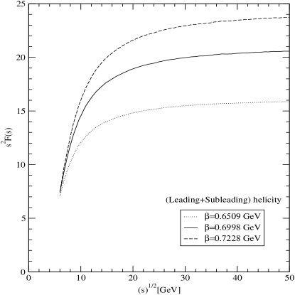
Figure 4: The form factor $s^{2}{\cal F}(s)$ for $e^{+}e^{-}\to J/\psi+\eta_{c}$. The dotted, short-dashed, long-dashed and solid line in left panel represent the peaking, leading twist(LT), higher twist(HT) results with the leading helicty contributions and HT one with all helicity contributions, respectively. The dot-dashed and double-dot-dashed line represent the dominant subleading contributions. The right panel represents the HT results including all helicity contributions obtained from linear(dotted line), HO(solid line), and HO’(dashed line) model parameters, respectively.

In Fig. 4, we show $s^{2}{\cal F}(s)$ for $e^{+}e^{-}\to J/\psi+\eta_{c}$ process. The left panel of Fig. 4 shows the results obtained from the central value $\beta=0.6998$ GeV of our model parameters displaying different(leading and subleading) helicity contributions. The right panel of Fig. 4 shows the sensitivity of our model predictions with all helicity contributions when the gaussian model parameter $\beta$ changes as shown in Fig. 3. In the left panel, the dotted and short-dashed lines represent the results obtained from the non-relativistic peaking approximation ${\cal F}^{\delta}(s)$[ Eq. (47)] and the leading twist(LT) factorized form factor ${\cal F}^{\rm LT}(s)$[ Eq. (45)] taking into account the relative motion of valence quarks, respectively. The long-dashed line represents the higher twist(HT) nonfactorized form factor ${\cal F}^{\rm HT}(s)$[Eq. (III)] obtained by including the transverse momenta$({\bf k}_{\perp},{\bf l}_{\perp})$ both in the wave function and the hard scattering part. Note that ${\cal F}^{\delta}(s)$(dotted line), ${\cal F}^{\rm LT}(s)$(short-dashed line), and ${\cal F}^{\rm HT}(s)$(long-dashed line) are obtained from the leading helicity contributions. The solid line represents our full solution ${\cal F}^{\rm HT}_{\rm(\Delta H=0+\Delta H=1)}(s)$ including all(leading plus subleading) helicity contributions summarized in the Appendix A(Tables 4 and  5). Among the subleading helicity contributions, we find that only $\uparrow\uparrow\to\uparrow\uparrow$(dot-dashed line) and $(\uparrow\downarrow\to\uparrow\downarrow)+(\downarrow\uparrow\to\downarrow\uparrow)$(double-dot-dashed line) helicity contributions give a sizeable effects and other subleading helicity contributions are negligible. As shown in Fig. 4, we find that while $s^{2}{\cal F}^{\rm HT}_{\rm(\Delta H=0+\Delta H=1)}(s)$ is about 2 times larger than $s^{2}{\cal F}^{\delta}(s)$ but 10$\%$ smaller than $s^{2}{\cal F}^{\rm LT}(s)$ at $\sqrt{s}=10.6$ GeV. It is also interesting to note that our $s^{2}{\cal F}^{\rm HT}_{\rm(\Delta H=0+\Delta H=1)}(s)$ takes over $s^{2}{\cal F}^{\rm LT}(s)$ for $\sqrt{s}\gtrsim 13$ GeV region, although $s^{2}{\cal F}^{\rm HT}(s)$ with leading helicity components approaches to $s^{2}{\cal F}^{\rm LT}(s)$ as $s\to\infty$. As one can see from Fig. 4, the form factor obtained from our calculation shows ${\cal F}(s)\sim s^{-2}$ as $s\to\infty$ which is the expected QCD scaling behaviorMa ; JMY ; BF ; MMT ; CJ ; BJ for the transition form factor between pseudoscalar ($0^{-+}$) and vector ($1^{--}$) mesons.

Figure 5: The cross section for $e^{+}e^{-}\to J/\psi\eta_{c}$ with leading and subleading helicity contributions using the HO model parameters(left panel) and with all helicity contributions using the linear, HO, and HO’ model parameters(right panel).

In Fig.5, we show leading order in $\alpha_{s}$ contribution to the cross section for $e^{+}e^{-}\to J/\psi+\eta_{c}$. The left panel of Fig. 5 shows the results with leading and subleading helicity contributions using the HO model parameters. The right panel of Fig. 5 shows the sensitivity of our model predictions with all helicity contributions when the gaussian model parameter $\beta$ changes as shown in Figs. 3 and  4. The line codes are the same as in Fig. 4. As one can see from the left panel of Fig.5, our peaking approximation result(dotted line) is consistent with the previous NRQCD estimates in Refs. BJ03 ; LHC03 ; HKQ03 , which is an order of magnitude smaller than the experimental data Belle ; Babar . We should note from the left panel of of Fig.5 that our higher twist result(solid line) including all helicity contributions enhances the peaking approximation result by a factor of $3\sim 4$ at $\sqrt{s}=10.6$ GeV while it reduces that of the leading twist result by $20\%$. As discussed in Section III, our higher twist results ($\sigma_{\rm HT}$) include all orders of ${\bf k}^{2}_{\perp}/{\bf q}^{2}_{\perp}$, ${\bf l}^{2}_{\perp}/{\bf q}^{2}_{\perp}$ and ${\bf k}_{\perp}\cdot{\bf l}_{\perp}/{\bf q}^{2}_{\perp}$ to keep effectively all higher orders of the relative quark velocity beyond $\langle v^{2}\rangle$. If we keep only the leading order of these terms (${\bf k}^{2}_{\perp}/{\bf q}^{2}_{\perp}$, ${\bf l}^{2}_{\perp}/{\bf q}^{2}_{\perp}$ and ${\bf k}_{\perp}\cdot{\bf l}_{\perp}/{\bf q}^{2}_{\perp}$), our results would correspond to include the relativistic effects up to the order of $\langle v^{2}\rangle$EM . Our predictions for the cross section at $\sqrt{s}=10.6$ GeV obtained from peaking approximation($\sigma_{\delta}$), leading twist($\sigma_{\rm LT}$) and higher twist($\sigma_{\rm HT}$) are given by

$$\sigma_{\delta}(J/\psi+\eta_{c}) = 2.34^{+0.50}_{-0.69}[\rm fb],$$

$$\sigma_{\rm LT}(J/\psi+\eta_{c}) = 10.57^{+3.15}_{-4.02}[\rm fb],$$

$$\sigma^{(\Delta H=0+\Delta H=1)}_{\rm HT}(J/\psi+\eta_{c}) = 8.76^{+1.61}_{-2.84}[\rm fb],$$ (53)

where the central, upper and lower values are obtained from HO, HO^′ and linear potential parameters, respectively. Our prediction of $\sigma^{(\Delta H=0+\Delta H=1)}_{\rm HT}(J/\psi+\eta_{c})$ reduces by about $10\%$ from the value in Eq.(IV) to $7.68^{+1.94}_{-2.66}$[fb] when we keep only the leading order of ${\bf k}^{2}_{\perp}/{\bf q}^{2}_{\perp}$, ${\bf l}^{2}_{\perp}/{\bf q}^{2}_{\perp}$ and ${\bf k}_{\perp}\cdot{\bf l}_{\perp}/{\bf q}^{2}_{\perp}$. It is interesting to note that our reduced value $7.68^{+1.94}_{-2.66}$[fb] is indeed very close to the result $7.8[\rm fb]$ obtained in the recent investigation including the relativistic effects up to $\langle v^{2}\rangle$EM .

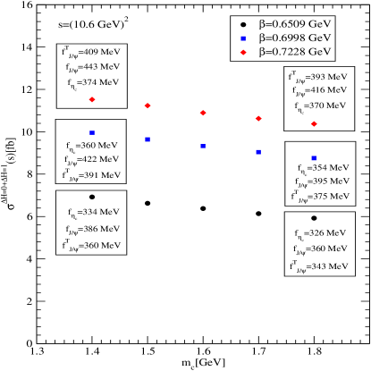
Figure 6: The parameter ($m_{c},\beta$) dependence of the cross section for $e^{+}e^{-}\to J/\psi+\eta_{c}$.

As a sensitivity check, we show in Fig. 6 the parameter ($m_{c},\beta$) dependence of the cross section for $e^{+}e^{-}\to J/\psi+\eta_{c}$ using the nonfactorized higher twist form factor with all helicty contributions. We also show in Fig. 6 the decay constants corresponding to the end point mass values, $m_{c}=1.4$ GeV and 1.8 GeV. The cross section increases as $\beta(m_{c})$ increases(decreases). As one can also see from Fig. 6, the cross section is more sensitive to the variation of the gaussian parameter than to the variation of the charm quark mass.

The experimental results are

$$\sigma(J/\psi+\eta_{c})\times B^{\eta_{c}}[\geq 2]=(25.6\pm 2.8\pm 3.4)[\rm fb],$$ (54)

by Belle Belle (filled circle in Fig 5) and

$$\sigma(J/\psi+\eta_{c})\times B^{\eta_{c}}[\geq 2]=(17.6\pm 2.8^{+1.5}_{-2.1})[\rm fb],$$ (55)

by Babar Babar (filled square in Fig 5), where $B^{\eta_{c}}[\geq 2]$ is the branching fraction for $\eta_{c}$ decay into at least two charged particles. Considering an enhancement by the factor of $1.8$ from the corrections of next-to-leading order (NLO) of $\alpha_{s}$ZGC , it might be conceivable to raise our leading $\alpha_{s}$ order result $\sigma^{(\Delta H=0+\Delta H=1)}_{\rm HT}(J/\psi+\eta_{c})$ in Eq.(IV) by this factor and get a value close to the above Babar data. However, it would be necessary to make detailed NLO investigation within the LF PQCD framework before we can make any firm conclusion.

V Summary and Conclusion

We investigated the transverse momentum effect on the exclusive charmonium $J/\psi+\eta_{c}$ pair production in $e^{+}e^{-}$ annihilation using the nonfactorized PQCD and LFQM that goes beyond the peaking approximation.

Our LFQM calculation based on the variational principle for the QCD-motivated Hamiltonian CJ1 ; CJ2 shows that the quark DAs for $J/\psi$ and $\eta_{c}$ take substantially broad shape which is quite different from the $\delta$-type DA. If the quark DA is not an exact $\delta$ function, i.e. the relative motion of valence quarks can play a significant role, the factorization theorem is no longer applicable. In going beyond the peaking approximation, we stressed a consistency by keeping the transverse momentum ${\bf k}_{\perp}$ both in the wave function part and the hard scattering part simultaneously before doing any integration in the amplitude. Such non-factorized analysis should be distinguished from the factorized analysis where the transverse momenta are seperately integrated out in the wave function part and in the hard scattering part. Even if the used LF wave functions lead to the similar shapes of DAs, predictions for the cross sections of double-charm productions are apparently different between the factorized and non-factorized analyses. We found that the higher twist contributions including all helicity contributions enhanced NRQCD result by a factor of $3\sim 4$ at $\sqrt{s}=10.6$ GeV while it reduced that of the leading twist result by $20\%$. We also found that the cross section for $e^{+}e^{-}\to J/\psi\eta_{c}$ process at $\sqrt{s}=10.6$ GeV is more sensitive to the variation of the gaussian parameter than to that of the charm quark mass. Our results showed that the cross section increases as $\beta(m_{c})$ increases(decreases).

In conclusion, LFQM/PQCD analysis showed that the relativistic correction(i.e. non-delta function) of the light-front wave function is very important to understand the large discrepancy between the NRQCD result and the experimental data given by Eqs.(54) and (55). While there have been considerations of broadening the quark DA to reduce the discrepancy between the theory at the leading order of $\alpha_{s}$ and the experimental resultsBC ; Ma ; BLL05 , a recent calculation of corrections of next-to-leading order(NLO) of $\alpha_{s}$ leads to an enhancement of the theoretical prediction by the factor about 1.8 ZGC . This factor may enhance our result in the leading order of $\alpha_{s}$ to fit the current experimental results. However, more detailed investigation is necessary prior to any firm conclusion on this issue.

Appendix A Helicity contributions to the hard scattering amplitude

In this appenix A, we summarize the helicity contributions $(\lambda_{1},\lambda_{2})\to(\lambda^{\prime}_{1},\lambda^{\prime}_{2})$ to the hard scattering amplitude $T^{(\lambda_{1},\lambda_{2})\to(\lambda^{\prime}_{1},\lambda^{\prime}_{2})}_{H}$ for the $\eta_{c}(P)\to\gamma^{*}(q)+J/\psi(P^{\prime})$ process.

Table 4: Helicity contributions to the hard scattering amplitude $T_{A}$ in Fig. 2.

$|\Delta H|$	Helicities	$N_{A_{1}}$	$N_{A_{2}}$	$N_{A_{3}}$	$\sum_{i}T_{A_{i}}(\Delta_{x}=\Delta_{y}=0)$
	$\uparrow\downarrow\to\uparrow\downarrow$	$P_{A1}+iQ_{A}$	$P_{A2}+iQ_{A}$	$P_{A3}+iQ_{A}$	$-\frac{8\pi\alpha_{s}C_{F}}{(y_{2}-x_{2})}[\frac{P_{A}+iQ}{{\cal D}_{1}{\cal D}_{2}}+\frac{2}{(y_{2}-x_{2}){\cal D}_{2}}]$
	$\downarrow\uparrow\to\downarrow\uparrow$	$P_{A1}-iQ_{A}$	$P_{A2}-iQ_{A}$	$P_{A3}-iQ_{A}$	$-\frac{8\pi\alpha_{s}C_{F}}{(y_{2}-x_{2})}[\frac{P_{A}-iQ}{{\cal D}_{1}{\cal D}_{2}}+\frac{2}{(y_{2}-x_{2}){\cal D}_{2}}]$
0	$\uparrow\downarrow\to\downarrow\uparrow$	$-\frac{2m^{2}(y_{1}-x_{1})(y_{2}-x_{2})}{x_{1}x_{2}y_{1}y_{2}}$	$N_{A_{1}}^{(\uparrow\downarrow\to\downarrow\uparrow)}$	$N_{A_{1}}^{(\uparrow\downarrow\to\downarrow\uparrow)}$	$-\frac{8\pi\alpha_{s}C_{F}}{(y_{2}-x_{2}){\cal D}_{1}{\cal D}_{2}}N_{A_{1}}^{(\uparrow\downarrow\to\downarrow\uparrow)}$
	$\downarrow\uparrow\to\uparrow\downarrow$	$-\frac{2m^{2}(y_{1}-x_{1})(y_{2}-x_{2})}{x_{1}x_{2}y_{1}y_{2}}$	$N_{A_{1}}^{(\downarrow\uparrow\to\uparrow\downarrow)}$	$N_{A_{1}}^{(\downarrow\uparrow\to\uparrow\downarrow)}$	$-\frac{8\pi\alpha_{s}C_{F}}{(y_{2}-x_{2}){\cal D}_{1}{\cal D}_{2}}N_{A_{1}}^{(\downarrow\uparrow\to\uparrow\downarrow)}$
	$\uparrow\uparrow\to\uparrow\uparrow$	$F_{A1}+iG_{A}$	$F_{A2}+iG_{A}$	$F_{A3}+iG_{A}$	$-\frac{8\pi\alpha_{s}C_{F}}{(y_{2}-x_{2})}[\frac{F_{A}+iG}{{\cal D}_{1}{\cal D}_{2}}+\frac{2}{(y_{2}-x_{2}){\cal D}_{2}}]$
	$\downarrow\downarrow\to\downarrow\downarrow$	$F_{A1}-iG_{A}$	$F_{A2}-iG_{A}$	$F_{A3}-iG_{A}$	$-\frac{8\pi\alpha_{s}C_{F}}{(y_{2}-x_{2})}[\frac{F_{A}-iG}{{\cal D}_{1}{\cal D}_{2}}+\frac{2}{(y_{2}-x_{2}){\cal D}_{2}}]$
	$\uparrow\downarrow\to\uparrow\uparrow$	$\frac{2m(x_{1}l-y_{1}k-x_{2}y_{1}q)^{L}}{x_{2}y_{1}y_{2}}$	$N_{A_{1}}^{(\uparrow\downarrow\to\uparrow\uparrow)}$	$N_{A_{1}}^{(\uparrow\downarrow\to\uparrow\uparrow)}$	$-\frac{8\pi\alpha_{s}C_{F}}{(y_{2}-x_{2}){\cal D}_{1}{\cal D}_{2}}N_{A_{1}}^{(\uparrow\downarrow\to\uparrow\uparrow)}$
	$\uparrow\downarrow\to\downarrow\downarrow$	$\frac{2m(x_{2}l-y_{2}k-x_{2}y_{2}q)^{R}}{x_{1}y_{1}y_{2}}$	$N_{A_{1}}^{(\uparrow\downarrow\to\downarrow\downarrow)}$	$N_{A_{1}}^{(\uparrow\downarrow\to\downarrow\downarrow)}$	$-\frac{8\pi\alpha_{s}C_{F}}{(y_{2}-x_{2}){\cal D}_{1}{\cal D}_{2}}N_{A_{1}}^{(\uparrow\downarrow\to\downarrow\downarrow)}$
	$\downarrow\uparrow\to\uparrow\uparrow$	$-\frac{2m(x_{2}l-y_{2}k-x_{2}y_{2}q)^{L}}{x_{1}y_{1}y_{2}}$	$N_{A_{1}}^{(\downarrow\uparrow\to\uparrow\uparrow)}$	$N_{A_{1}}^{(\downarrow\uparrow\to\uparrow\uparrow)}$	$-\frac{8\pi\alpha_{s}C_{F}}{(y_{2}-x_{2}){\cal D}_{1}{\cal D}_{2}}N_{A_{1}}^{(\downarrow\uparrow\to\uparrow\uparrow)}$
1	$\downarrow\uparrow\to\downarrow\downarrow$	$-\frac{2m(x_{1}l-y_{1}k-x_{2}y_{1}q)^{R}}{x_{2}y_{1}y_{2}}$	$N_{A_{1}}^{(\downarrow\uparrow\to\downarrow\downarrow)}$	$N_{A_{1}}^{(\downarrow\uparrow\to\downarrow\downarrow)}$	$-\frac{8\pi\alpha_{s}C_{F}}{(y_{2}-x_{2}){\cal D}_{1}{\cal D}_{2}}N_{A_{1}}^{(\downarrow\uparrow\to\downarrow\downarrow)}$
	$\uparrow\uparrow\to\uparrow\downarrow$	$-\frac{2m(x_{1}l-y_{1}k-x_{2}y_{1}q)^{R}}{x_{1}x_{2}y_{2}}$	$N_{A_{1}}^{(\uparrow\uparrow\to\uparrow\downarrow)}$	$N_{A_{1}}^{(\uparrow\uparrow\to\uparrow\downarrow)}$	$-\frac{8\pi\alpha_{s}C_{F}}{(y_{2}-x_{2}){\cal D}_{1}{\cal D}_{2}}N_{A_{1}}^{(\uparrow\uparrow\to\uparrow\downarrow)}$
	$\downarrow\downarrow\to\uparrow\downarrow$	$-\frac{2m(x_{2}l-y_{2}k-x_{2}y_{2}q)^{L}}{x_{1}x_{2}y_{1}}$	$N_{A_{1}}^{(\downarrow\downarrow\to\uparrow\downarrow)}$	$N_{A_{1}}^{(\downarrow\downarrow\to\uparrow\downarrow)}$	$-\frac{8\pi\alpha_{s}C_{F}}{(y_{2}-x_{2}){\cal D}_{1}{\cal D}_{2}}N_{A_{1}}^{(\downarrow\downarrow\to\uparrow\downarrow)}$
	$\uparrow\uparrow\to\downarrow\uparrow$	$\frac{2m(x_{2}l-y_{2}k-x_{2}y_{2}q)^{R}}{x_{1}x_{2}y_{1}}$	$N_{A_{1}}^{(\uparrow\uparrow\to\downarrow\uparrow)}$	$N_{A_{1}}^{(\uparrow\uparrow\to\downarrow\uparrow)}$	$-\frac{8\pi\alpha_{s}C_{F}}{(y_{2}-x_{2}){\cal D}_{1}{\cal D}_{2}}N_{A_{1}}^{(\uparrow\uparrow\to\downarrow\uparrow)}$
	$\downarrow\downarrow\to\downarrow\uparrow$	$\frac{2m(x_{1}l-y_{1}k-x_{2}y_{1}q)^{L}}{x_{1}x_{2}y_{2}}$	$N_{A_{1}}^{(\downarrow\downarrow\to\downarrow\uparrow)}$	$N_{A_{1}}^{(\downarrow\downarrow\to\downarrow\uparrow)}$	$-\frac{8\pi\alpha_{s}C_{F}}{(y_{2}-x_{2}){\cal D}_{1}{\cal D}_{2}}N_{A_{1}}^{(\downarrow\downarrow\to\downarrow\uparrow)}$
2	$\uparrow\uparrow\to\downarrow\downarrow$	0	0	0	0
	$\downarrow\downarrow\to\uparrow\uparrow$	0	0	0	0

Table 5: Helicity contributions to the hard scattering amplitude $T_{B}$ in Fig. 2.

$|\Delta H|$	Helicities	$N_{B_{1}}$	$N_{B_{2}}$	$N_{B_{3}}$	$\sum_{i}T_{B_{i}}(\Delta_{x}=\Delta_{y}=0)$
	$\uparrow\downarrow\to\uparrow\downarrow$	$P_{B1}+iQ_{B}$	$P_{B2}+iQ_{B}$	$P_{B3}+iQ_{B}$	$-\frac{8\pi\alpha_{s}C_{F}}{(y_{2}-x_{2})}[\frac{P_{B}+iQ_{B}}{{\cal D}_{2}{\cal D}_{8}}+\frac{2}{(y_{2}-x_{2}){\cal D}_{5}}]$
	$\downarrow\uparrow\to\downarrow\uparrow$	$P_{B1}-iQ_{B}$	$P_{B2}-iQ_{B}$	$P_{B3}-iQ_{B}$	$-\frac{8\pi\alpha_{s}C_{F}}{(y_{2}-x_{2})}[\frac{P_{B}-iQ_{B}}{{\cal D}_{2}{\cal D}_{8}}+\frac{2}{(y_{2}-x_{2}){\cal D}_{5}}]$
0	$\uparrow\downarrow\to\downarrow\uparrow$	$-\frac{2m^{2}(y_{1}-x_{1})(y_{2}-x_{2})}{x_{1}x_{2}y_{1}y_{2}}$	$N_{B_{1}}^{(\uparrow\downarrow\to\downarrow\uparrow)}$	$N_{B_{1}}^{(\uparrow\downarrow\to\downarrow\uparrow)}$	$-\frac{8\pi\alpha_{s}C_{F}}{(y_{2}-x_{2}){\cal D}_{2}{\cal D}_{8}}N_{B_{1}}^{(\uparrow\downarrow\to\downarrow\uparrow)}$
	$\downarrow\uparrow\to\uparrow\downarrow$	$-\frac{2m^{2}(y_{1}-x_{1})(y_{2}-x_{2})}{x_{1}x_{2}y_{1}y_{2}}$	$N_{B_{1}}^{(\downarrow\uparrow\to\uparrow\downarrow)}$	$N_{B_{1}}^{(\downarrow\uparrow\to\uparrow\downarrow)}$	$-\frac{8\pi\alpha_{s}C_{F}}{(y_{2}-x_{2}){\cal D}_{2}{\cal D}_{8}}N_{B_{1}}^{(\downarrow\uparrow\to\uparrow\downarrow)}$
	$\uparrow\uparrow\to\uparrow\uparrow$	$F_{B1}+iG_{B}$	$F_{B2}+iG_{B}$	$F_{B3}+iG_{B}$	$-\frac{8\pi\alpha_{s}C_{F}}{(y_{2}-x_{2})}[\frac{F_{B}+iG_{B}}{{\cal D}_{2}{\cal D}_{8}}+\frac{2}{(y_{2}-x_{2}){\cal D}_{5}}]$
	$\downarrow\downarrow\to\downarrow\downarrow$	$F_{B1}-iG_{B}$	$F_{B2}-iG_{B}$	$F_{B3}-iG_{B}$	$-\frac{8\pi\alpha_{s}C_{F}}{(y_{2}-x_{2})}[\frac{F_{B}-iG_{B}}{{\cal D}_{2}{\cal D}_{8}}+\frac{2}{(y_{2}-x_{2}){\cal D}_{5}}]$
	$\uparrow\downarrow\to\uparrow\uparrow$	$\frac{2m(x_{1}l-y_{1}k-x_{1}y_{2}q)^{L}}{x_{2}y_{1}y_{2}}$	$N_{B_{1}}^{(\uparrow\downarrow\to\uparrow\uparrow)}$	$N_{B_{1}}^{(\uparrow\downarrow\to\uparrow\uparrow)}$	$-\frac{8\pi\alpha_{s}C_{F}}{(y_{2}-x_{2}){\cal D}_{2}{\cal D}_{8}}N_{B_{1}}^{(\uparrow\downarrow\to\uparrow\uparrow)}$
	$\uparrow\downarrow\to\downarrow\downarrow$	$\frac{2m(x_{2}l-y_{2}k-x_{2}y_{2}q)^{R}}{x_{1}y_{1}y_{2}}$	$N_{B_{1}}^{(\uparrow\downarrow\to\downarrow\downarrow)}$	$N_{B_{1}}^{(\uparrow\downarrow\to\downarrow\downarrow)}$	$-\frac{8\pi\alpha_{s}C_{F}}{(y_{2}-x_{2}){\cal D}_{2}{\cal D}_{8}}N_{B_{1}}^{(\uparrow\downarrow\to\downarrow\downarrow)}$
	$\downarrow\uparrow\to\uparrow\uparrow$	$-\frac{2m(x_{2}l-y_{2}k-x_{2}y_{2}q)^{L}}{x_{1}y_{1}y_{2}}$	$N_{B_{1}}^{(\downarrow\uparrow\to\uparrow\uparrow)}$	$N_{B_{1}}^{(\downarrow\uparrow\to\uparrow\uparrow)}$	$-\frac{8\pi\alpha_{s}C_{F}}{(y_{2}-x_{2}){\cal D}_{2}{\cal D}_{8}}N_{B_{1}}^{(\downarrow\uparrow\to\uparrow\uparrow)}$
1	$\downarrow\uparrow\to\downarrow\downarrow$	$-\frac{2m(x_{1}l-y_{1}k-x_{1}y_{2}q)^{R}}{x_{2}y_{1}y_{2}}$	$N_{B_{1}}^{(\downarrow\uparrow\to\downarrow\downarrow)}$	$N_{B_{1}}^{(\downarrow\uparrow\to\downarrow\downarrow)}$	$-\frac{8\pi\alpha_{s}C_{F}}{(y_{2}-x_{2}){\cal D}_{2}{\cal D}_{8}}N_{B_{1}}^{(\downarrow\uparrow\to\downarrow\downarrow)}$
	$\uparrow\uparrow\to\uparrow\downarrow$	$-\frac{2m(x_{1}l-y_{1}k-x_{1}y_{2}q)^{R}}{x_{1}x_{2}y_{2}}$	$N_{B_{1}}^{(\uparrow\uparrow\to\uparrow\downarrow)}$	$N_{B_{1}}^{(\uparrow\uparrow\to\uparrow\downarrow)}$	$-\frac{8\pi\alpha_{s}C_{F}}{(y_{2}-x_{2}){\cal D}_{2}{\cal D}_{8}}N_{B_{1}}^{(\uparrow\uparrow\to\uparrow\downarrow)}$
	$\downarrow\downarrow\to\uparrow\downarrow$	$-\frac{2m(x_{2}l-y_{2}k-x_{2}y_{2}q)^{L}}{x_{1}x_{2}y_{1}}$	$N_{B_{1}}^{(\downarrow\downarrow\to\uparrow\downarrow)}$	$N_{B_{1}}^{(\downarrow\downarrow\to\uparrow\downarrow)}$	$-\frac{8\pi\alpha_{s}C_{F}}{(y_{2}-x_{2}){\cal D}_{2}{\cal D}_{8}}N_{B_{1}}^{(\downarrow\downarrow\to\uparrow\downarrow)}$
	$\uparrow\uparrow\to\downarrow\uparrow$	$\frac{2m(x_{2}l-y_{2}k-x_{2}y_{2}q)^{R}}{x_{1}x_{2}y_{1}}$	$N_{B_{1}}^{(\uparrow\uparrow\to\downarrow\uparrow)}$	$N_{B_{1}}^{(\uparrow\uparrow\to\downarrow\uparrow)}$	$-\frac{8\pi\alpha_{s}C_{F}}{(y_{2}-x_{2}){\cal D}_{2}{\cal D}_{8}}N_{B_{1}}^{(\uparrow\uparrow\to\downarrow\uparrow)}$
	$\downarrow\downarrow\to\downarrow\uparrow$	$\frac{2m(x_{1}l-y_{1}k-x_{1}y_{2}q)^{L}}{x_{1}x_{2}y_{2}}$	$N_{B_{1}}^{(\downarrow\downarrow\to\downarrow\uparrow)}$	$N_{B_{1}}^{(\downarrow\downarrow\to\downarrow\uparrow)}$	$-\frac{8\pi\alpha_{s}C_{F}}{(y_{2}-x_{2}){\cal D}_{2}{\cal D}_{8}}N_{B_{1}}^{(\downarrow\downarrow\to\downarrow\uparrow)}$
2	$\uparrow\uparrow\to\downarrow\downarrow$	0	0	0	0
	$\downarrow\downarrow\to\uparrow\uparrow$	0	0	0	0

In Tables 4 and 5, we summarize our results for the helicity contributions to the hard scattering amplitudes $T_{A}$ and $T_{B}$ for the diagrams in Fig. 2, where

$$P_{A1} = \frac{-2}{x_{1}x_{2}y_{1}y_{2}}\biggl{[}x^{2}_{2}y_{1}y_{2}{\bf q}^{2}_{\perp}+x_{1}x_{2}{\bf l}^{2}_{\perp}+y_{1}y_{2}{\bf k}^{2}_{\perp}+x_{2}(x_{1}y_{1}+x_{2}y_{2})({\bf l}_{\perp}\cdot{\bf q}_{\perp})$$

$$+2x_{2}y_{1}y_{2}({\bf k}_{\perp}\cdot{\bf q}_{\perp})+(x_{1}y_{1}+x_{2}y_{2})(m^{2}+{\bf k}_{\perp}\cdot{\bf l}_{\perp})\biggr{]}+\frac{2}{(x_{1}-y_{1})}[D_{2}+D_{4}]=P_{A}+\frac{2}{(x_{1}-y_{1})}[D_{2}+D_{4}],$$

$$P_{A2} = P_{A}+\frac{2}{(x_{1}-y_{1})}[D_{2}+D_{4}],\;\;P_{A3}=P_{A}+\frac{2}{(x_{1}-y_{1})}[D_{2}-D_{4}],$$

$$Q_{A} = \frac{2}{x_{1}x_{2}y_{1}y_{2}}\biggl{[}x_{2}(x_{1}-y_{2})|{\bf l}_{\perp}\times{\bf q}_{\perp}|-2x_{1}y_{1}y_{2}|{\bf k}_{\perp}\times{\bf q}_{\perp}|+(x_{2}y_{2}+x_{1}y_{1})|{\bf k}_{\perp}\times{\bf l}_{\perp}|\biggl{]},$$

$$F_{A1} = \frac{-2}{x_{1}x_{2}y_{1}y_{2}}\biggl{[}{\bf k}_{\perp}\cdot{\bf l}_{\perp}+x_{2}({\bf l}_{\perp}\cdot{\bf q}_{\perp})+(x_{1}y_{1}+x_{2}y_{2})m^{2}\biggr{]}+\frac{2}{(x_{1}-y_{1})}[D_{2}+D_{4}]=F_{A}+\frac{2}{(x_{1}-y_{1})}[D_{2}+D_{4}],$$

$$F_{A2} = F_{A}+\frac{2}{(x_{1}-y_{1})}[D_{2}+D_{4}],\;\;F_{A3}=F_{A}+\frac{2}{(x_{1}-y_{1})}[D_{2}-D_{4}],$$

$$G_{A} = \frac{2}{x_{1}x_{2}y_{1}y_{2}}\biggl{[}2x_{1}y_{1}y_{2}|{\bf k}_{\perp}\times{\bf q}_{\perp}|-x_{2}|{\bf l}_{\perp}\times{\bf q}_{\perp}|+(1-2x_{1}y_{1})|{\bf k}_{\perp}\times{\bf l}_{\perp}|\biggr{]},$$ (56)

for the diagrams $A_{i}$ and

$$P_{B1} = \frac{-2}{x_{1}x_{2}y_{1}y_{2}}\biggl{[}x_{1}x_{2}y^{2}_{2}{\bf q}^{2}_{\perp}+x_{1}x_{2}{\bf l}^{2}_{\perp}+y_{1}y_{2}{\bf k}^{2}_{\perp}-y_{2}(x_{1}y_{1}+x_{2}y_{2})({\bf k}_{\perp}\cdot{\bf q}_{\perp})$$

$$-2x_{1}x_{2}y_{2}({\bf l}_{\perp}\cdot{\bf q}_{\perp})+(x_{1}y_{1}+x_{2}y_{2})(m^{2}+{\bf k}_{\perp}\cdot{\bf l}_{\perp})\biggr{]}+\frac{2}{(y_{2}-x_{2})}[D_{9}+D_{7}]=P_{B}+\frac{2}{(y_{2}-x_{2})}[D_{9}+D_{7}],$$

$$P_{B2} = P_{B}+\frac{2}{(x_{2}-y_{2})}[D_{9}+D_{7}],\;\;P_{B3}=P_{B}+\frac{2}{(y_{2}-x_{2})}[D_{9}-D_{7}],$$

$$Q_{B} = \frac{2}{x_{1}x_{2}y_{1}y_{2}}(x_{1}y_{1}-x_{2}y_{2})(|{\bf l}_{\perp}\times{\bf k}_{\perp}|-y_{2}|{\bf q}_{\perp}\times{\bf k}_{\perp}|),$$

$$F_{B1} = \frac{-2}{x_{1}x_{2}y_{1}y_{2}}\biggl{[}{\bf k}_{\perp}\cdot{\bf l}_{\perp}-y_{2}({\bf k}_{\perp}\cdot{\bf q}_{\perp})+(x_{1}y_{1}+x_{2}y_{2})m^{2}\biggr{]}+\frac{2}{(y_{2}-x_{2})}[D_{9}+D_{7}]=F_{B}+\frac{2}{(y_{2}-x_{2})}[D_{9}+D_{7}],$$

$$F_{B2} = F_{B}+\frac{2}{(x_{2}-y_{2})}[D_{9}+D_{7}],\;\;F_{B3}=F_{B}+\frac{2}{(y_{2}-x_{2})}[D_{9}-D_{7}],$$

$$G_{B} = \frac{2}{x_{1}x_{2}y_{1}y_{2}}(y_{2}|{\bf q}_{\perp}\times{\bf k}_{\perp}|-|{\bf l}_{\perp}\times{\bf k}_{\perp}|),$$ (57)

for the diagrams $B_{i}$, respectively.

As an illustration, we show how to obtain the hard scattering amplitudes $T_{A}=\sum^{3}_{i=1}T_{A_{i}}$ (sixth column in Table 4) and $T_{B}=\sum^{3}_{i=1}T_{B_{i}}$(sixth column in Table 5) as well as the total amplitude $T_{H}=T_{A}+T_{B}$ for the $(\uparrow\downarrow\to\uparrow\downarrow)$ contribution. Using the identities Eqs. (38) and (III) in Sec.III, we obtain

$$\biggl{[}\sum_{i}T_{A_{i}}^{(\uparrow\downarrow\to\uparrow\downarrow)}\biggr{]}_{\Delta=0} = -8\pi\alpha_{s}C_{F}\biggl{[}\frac{\theta(y_{2}-x_{2})(P_{A1}+iQ_{A})}{(y_{2}-x_{2}){\cal D}_{1}{\cal D}_{2}}+\frac{\theta(x_{2}-y_{2})(P_{A2}+iQ_{A})}{(x_{2}-y_{2}){\cal D}_{3}{\cal D}_{4}}+\frac{\theta(x_{2}-y_{2})(P_{A3}+iQ_{A})}{(x_{2}-y_{2}){\cal D}_{5}{\cal D}_{6}}\biggr{]}$$ (58)

$$= -8\pi\alpha_{s}C_{F}(P_{A}+iQ_{A})\biggl{[}\frac{\theta(y_{2}-x_{2})}{(y_{2}-x_{2}){\cal D}_{1}{\cal D}_{2}}+\frac{\theta(x_{2}-y_{2})}{(x_{2}-y_{2})}\biggl{(}\frac{1}{{\cal D}_{3}{\cal D}_{4}}+\frac{1}{{\cal D}_{5}{\cal D}_{6}}\biggr{)}\biggr{]}$$

$$-16\pi\alpha_{s}C_{F}\biggl{[}\frac{\theta(y_{2}-x_{2})}{(y_{2}-x_{2})^{2}}\frac{{\cal D}_{2}+{\cal D}_{4}}{{\cal D}_{1}{\cal D}_{2}}+\frac{\theta(x_{2}-y_{2})}{(x_{2}-y_{2})^{2}}\biggl{(}\frac{{\cal D}_{2}+{\cal D}_{4}}{{\cal D}_{3}{\cal D}_{4}}+\frac{{\cal D}_{2}-{\cal D}_{4}}{{\cal D}_{5}{\cal D}_{6}}\biggr{)}\biggr{]}$$

$$= -8\pi\alpha_{s}C_{F}(P_{A}+iQ_{A})\biggl{[}\frac{1}{(y_{2}-x_{2}){\cal D}_{1}{\cal D}_{2}}\biggr{]}-8\pi\alpha_{s}C_{F}\biggl{[}\frac{2}{(y_{2}-x_{2})^{2}{\cal D}_{2}}\biggr{]},$$

and

$$\biggl{[}\sum_{i}T_{B_{i}}^{(\uparrow\downarrow\to\uparrow\downarrow)}\biggr{]}_{\Delta=0} = -8\pi\alpha_{s}C_{F}\biggl{[}\frac{\theta(y_{2}-x_{2})(P_{B_{1}}+iQ_{B})}{(y_{2}-x_{2}){\cal D}_{7}{\cal D}_{8}}+\frac{\theta(y_{2}-x_{2})(P_{B3}+iQ_{B})}{(y_{2}-x_{2}){\cal D}_{11}{\cal D}_{12}}+\frac{\theta(x_{2}-y_{2})(P_{B2}+iQ_{B})}{(x_{2}-y_{2}){\cal D}_{9}{\cal D}_{10}}\biggr{]}$$ (59)

$$= -8\pi\alpha_{s}C_{F}(P_{B}+iQ_{B})\biggl{[}\frac{\theta(y_{2}-x_{2})}{(y_{2}-x_{2})}\biggl{(}\frac{1}{{\cal D}_{7}{\cal D}_{8}}+\frac{1}{{\cal D}_{11}{\cal D}_{12}}\biggr{)}+\frac{\theta(x_{2}-y_{2})}{(x_{2}-y_{2}){\cal D}_{9}{\cal D}_{10}}\biggr{]}$$

$$-16\pi\alpha_{s}C_{F}\biggl{[}\frac{\theta(y_{2}-x_{2})}{(y_{2}-x_{2})^{2}}\biggl{(}\frac{{\cal D}_{9}+{\cal D}_{7}}{{\cal D}_{7}{\cal D}_{8}}+\frac{{\cal D}_{9}-{\cal D}_{7}}{{\cal D}_{11}{\cal D}_{12}}\biggr{)}+\frac{\theta(x_{2}-y_{2})}{(x_{2}-y_{2})^{2}}\frac{{\cal D}_{9}+{\cal D}_{7}}{{\cal D}_{9}{\cal D}_{10}}\biggr{]}$$

$$= -8\pi\alpha_{s}C_{F}(P_{B}+iQ_{B})\biggl{[}\frac{1}{(y_{2}-x_{2}){\cal D}_{2}{\cal D}_{8}}\biggr{]}-8\pi\alpha_{s}C_{F}\biggl{[}\frac{2}{(y_{2}-x_{2})^{2}{\cal D}_{5}}\biggr{]},$$

where the first terms in Eqs. (58) and (59) proportional to $1/(y_{2}-x_{2})$ and the second terms proportional to $1/(y_{2}-x_{2})^{2}$ are related with the Feynman gauge and the LF gauge parts, respectively. By adding all six LF time-ordered diagrams, we obtain

$$T_{H}^{(\uparrow\downarrow\to\uparrow\downarrow)} = \sum_{i}\biggl{[}T_{A_{i}}^{(\uparrow\downarrow\to\uparrow\downarrow)}+T_{B_{i}}^{(\uparrow\downarrow\to\uparrow\downarrow)}\biggr{]}_{\Delta=0}$$

$$= -\frac{8\pi\alpha_{s}C_{F}}{(y_{2}-x_{2})}\biggl{[}\frac{(P_{A}+iQ)}{{\cal D}_{1}{\cal D}_{2}}+\frac{(P_{B}+iQ_{B})}{{\cal D}_{2}{\cal D}_{8}}\biggr{]},$$

i.e. the singular LF gauge parts cancel each other and only finite Feynman gauge parts contribute to the amplitude. Similarly, we obtain other helicity contributions to the hard scattering amplitude as shown in Tables 4 and 5.

Appendix B Hard scattering amplitude combined with Relativistic Spin-orbit wave function

In this appendix B, we list the leading and subleading helicity contributions to the hard scattering amplitude combined with the relativistic spin-orbit wave function, where the subleading helicity contributions show up as next-to-leading order in transverse momenta. That is, the subleading helicity contributions vanish at leading twist.

We first consider the relativistic spin-orbit wave functions for pseudoscalar and vector(with transverse polarization $\epsilon=+1$) mesons given by Eqs. (4) and (6), respectively. Besides the leading helicity(in tranverse momenta) contributions coming from two $\Delta H=1$ contributions(i.e. $\uparrow\downarrow\to\uparrow\uparrow$ and $\downarrow\uparrow\to\uparrow\uparrow$), the subleading helicity contributions are as follows.

(1) $\Delta H=0$ contributions:

$${\cal R}^{11\dagger}_{\uparrow\downarrow}{\cal R}^{00}_{\uparrow\downarrow} = \frac{m\sqrt{2}}{C_{x}C_{y}}\biggl{[}\frac{y_{1}M_{0y}+m}{M_{0y}+2m}\biggr{]}l^{L}=-{\cal R}^{11\dagger}_{\uparrow\downarrow}{\cal R}^{00}_{\downarrow\uparrow},$$

$${\cal R}^{11\dagger}_{\downarrow\uparrow}{\cal R}^{00}_{\downarrow\uparrow} = \frac{m\sqrt{2}}{C_{x}C_{y}}\biggl{[}\frac{y_{2}M_{0y}+m}{M_{0y}+2m}\biggr{]}l^{L}=-{\cal R}^{11\dagger}_{\downarrow\uparrow}{\cal R}^{00}_{\uparrow\downarrow},$$

$${\cal R}^{11\dagger}_{\uparrow\uparrow}{\cal R}^{00}_{\uparrow\uparrow} = -\frac{\sqrt{2}}{C_{x}C_{y}}\biggl{[}m+\frac{{\bf l}^{2}_{\perp}}{M_{0y}+2m}\biggr{]}k^{L}$$

$${\cal R}^{11\dagger}_{\downarrow\downarrow}{\cal R}^{00}_{\downarrow\downarrow} = \frac{\sqrt{2}}{C_{x}C_{y}}\biggl{[}\frac{1}{M_{0y}+2m}\biggr{]}k^{R}(l^{L})^{2}.$$ (61)

(2) $\Delta H=1$ contributions:

$${\cal R}^{11\dagger}_{\downarrow\downarrow}{\cal R}^{00}_{\downarrow\uparrow} = \frac{m\sqrt{2}}{C_{x}C_{y}}\biggl{[}\frac{1}{M_{0y}+2m}\biggr{]}(l^{L})^{2}=-{\cal R}^{11\dagger}_{\downarrow\downarrow}{\cal R}^{00}_{\uparrow\downarrow},$$

$${\cal R}^{11\dagger}_{\uparrow\downarrow}{\cal R}^{00}_{\uparrow\uparrow} = -\frac{\sqrt{2}}{C_{x}C_{y}}\biggl{[}\frac{y_{1}M_{0y}+m}{M_{0y}+2m}\biggr{]}l^{L}k^{L},$$

$${\cal R}^{11\dagger}_{\uparrow\downarrow}{\cal R}^{00}_{\downarrow\downarrow} = -\frac{\sqrt{2}}{C_{x}C_{y}}\biggl{[}\frac{y_{1}M_{0y}+m}{M_{0y}+2m}\biggr{]}l^{L}k^{R},$$

$${\cal R}^{11\dagger}_{\downarrow\uparrow}{\cal R}^{00}_{\uparrow\uparrow} = \frac{\sqrt{2}}{C_{x}C_{y}}\biggl{[}\frac{y_{2}M_{0y}+m}{M_{0y}+2m}\biggr{]}l^{L}k^{L},$$

$${\cal R}^{11\dagger}_{\downarrow\uparrow}{\cal R}^{00}_{\downarrow\downarrow} = \frac{\sqrt{2}}{C_{x}C_{y}}\biggl{[}\frac{y_{2}M_{0y}+m}{M_{0y}+2m}\biggr{]}l^{L}k^{R}.$$ (62)

where $C_{x}=\sqrt{2x_{1}x_{2}}M_{0x}$ and $C_{y}=\sqrt{2y_{1}y_{2}}M_{0y}$. Since the hard scattering amplitudes vanish for $\Delta H=2$ cases, we do not consider them here.

Next, we obtain the hard scattering amplitude combined with the spin-orbit wave function.

(1) $\Delta H=0$ contributions:

$${\cal T}^{R}_{H}(\uparrow\downarrow\to\uparrow\downarrow) = \frac{\sqrt{2}}{q^{L}}{\cal R}^{11\dagger}_{\uparrow\downarrow}T^{(\uparrow\downarrow\to\uparrow\downarrow)}_{H}{\cal R}^{00}_{\uparrow\downarrow}$$

$$= \frac{16\pi\alpha_{s}C_{F}m}{(y_{2}-x_{2})C_{x}C_{y}q^{2}}\biggl{[}\frac{y_{1}M_{0y}+m}{M_{0y}+2m}\biggr{]}$$

$$\times(l^{L}q^{R})\biggl{[}\frac{P_{A}+iQ_{A}}{{\cal D}_{1}{\cal D}_{2}}+\frac{P_{B}+iQ_{B}}{{\cal D}_{2}{\cal D}_{8}}\biggr{]},$$

$${\cal T}^{R}_{H}(\downarrow\uparrow\to\downarrow\uparrow) = \frac{\sqrt{2}}{q^{L}}{\cal R}^{11\dagger}_{\downarrow\uparrow}T^{(\downarrow\uparrow\to\downarrow\uparrow)}_{H}{\cal R}^{00}_{\downarrow\uparrow}$$

$$= \frac{16\pi\alpha_{s}C_{F}m}{(y_{2}-x_{2})C_{x}C_{y}q^{2}}\biggl{[}\frac{y_{2}M_{0y}+m}{M_{0y}+2m}\biggr{]}$$

$$\times(l^{L}q^{R})\biggl{[}\frac{P_{A}-iQ_{A}}{{\cal D}_{1}{\cal D}_{2}}+\frac{P_{B}-iQ_{B}}{{\cal D}_{2}{\cal D}_{8}}\biggr{]},$$

$${\cal T}^{R}_{H}(\uparrow\uparrow\to\uparrow\uparrow) = \frac{\sqrt{2}}{q^{L}}{\cal R}^{11\dagger}_{\uparrow\uparrow}T^{(\uparrow\uparrow\to\uparrow\uparrow)}_{H}{\cal R}^{00}_{\uparrow\uparrow}$$

$$= \frac{-16\pi\alpha_{s}C_{F}}{(y_{2}-x_{2})C_{x}C_{y}q^{2}}\biggl{[}m+\frac{{\bf l}^{2}_{\perp}}{M_{0y}+2m}\biggr{]}$$

$$\times(k^{L}q^{R})\biggl{[}\frac{F_{A}+iG_{A}}{{\cal D}_{1}{\cal D}_{2}}+\frac{F_{B}+iG_{B}}{{\cal D}_{2}{\cal D}_{8}}\biggr{]},$$

$${\cal T}^{R}_{H}(\downarrow\downarrow\to\downarrow\downarrow) = \frac{\sqrt{2}}{q^{L}}{\cal R}^{11\dagger}_{\downarrow\downarrow}T^{(\downarrow\downarrow\to\downarrow\downarrow)}_{H}{\cal R}^{00}_{\downarrow\downarrow}$$

$$= \frac{16\pi\alpha_{s}C_{F}}{(y_{2}-x_{2})C_{x}C_{y}q^{2}}\biggl{[}\frac{1}{M_{0y}+2m}\biggr{]}$$

$$\times(k^{R}l^{L}l^{L}q^{R})\biggl{[}\frac{F_{A}-iG_{A}}{{\cal D}_{1}{\cal D}_{2}}+\frac{F_{B}-iG_{B}}{{\cal D}_{2}{\cal D}_{8}}\biggr{]},$$

$${\cal T}^{R}_{H}(\uparrow\downarrow\to\downarrow\uparrow) = \frac{\sqrt{2}}{q^{L}}{\cal R}^{11\dagger}_{\downarrow\uparrow}T^{(\uparrow\downarrow\to\downarrow\uparrow)}_{H}{\cal R}^{00}_{\uparrow\downarrow}$$ (67)

$$= \frac{32\pi\alpha_{s}C_{F}m^{3}(y_{1}-x_{1})}{x_{1}x_{2}y_{1}y_{2}C_{x}C_{y}q^{2}}\biggl{[}\frac{y_{2}M_{0y}+m}{M_{0y}+2m}\biggr{]}$$

$$\times(l^{L}q^{R})\biggl{[}\frac{1}{{\cal D}_{1}{\cal D}_{2}}+\frac{1}{{\cal D}_{2}{\cal D}_{8}}\biggr{]},$$

$${\cal T}^{R}_{H}(\downarrow\uparrow\to\uparrow\downarrow) = \frac{\sqrt{2}}{q^{L}}{\cal R}^{11\dagger}_{\uparrow\downarrow}T^{(\downarrow\uparrow\to\uparrow\downarrow)}_{H}{\cal R}^{00}_{\downarrow\uparrow}$$ (68)

$$= \frac{32\pi\alpha_{s}C_{F}m^{3}(y_{1}-x_{1})}{x_{1}x_{2}y_{1}y_{2}C_{x}C_{y}q^{2}}\biggl{[}\frac{y_{1}M_{0y}+m}{M_{0y}+2m}\biggr{]}$$

$$\times(l^{L}q^{R})\biggl{[}\frac{1}{{\cal D}_{1}{\cal D}_{2}}+\frac{1}{{\cal D}_{2}{\cal D}_{8}}\biggr{]}.$$

(2) $\Delta H=1$ contributions:

$${\cal T}^{R}_{H}(\uparrow\downarrow\to\downarrow\downarrow) = \frac{\sqrt{2}}{q^{L}}{\cal R}^{11\dagger}_{\downarrow\downarrow}T^{(\uparrow\downarrow\to\downarrow\downarrow)}_{H}{\cal R}^{00}_{\uparrow\downarrow}$$ (69)

$$= \frac{-32\pi\alpha_{s}C_{F}m^{2}}{x_{1}y_{1}y_{2}(y_{2}-x_{2})C_{x}C_{y}q^{2}}\biggl{[}\frac{1}{M_{0y}+2m}\biggr{]}$$

$$\times(l^{L}q^{R})\biggl{[}\frac{x_{2}{\bf l}^{2}_{\perp}-y_{2}l^{L}k^{R}-x_{2}y_{2}l^{L}q^{R}}{{\cal D}_{1}{\cal D}_{2}}$$

$$+\frac{x_{2}{\bf l}^{2}_{\perp}-y_{2}l^{L}k^{R}-x_{2}y_{2}l^{L}q^{R}}{{\cal D}_{2}{\cal D}_{8}}\biggr{]},$$

$${\cal T}^{R}_{H}(\downarrow\uparrow\to\downarrow\downarrow) = \frac{\sqrt{2}}{q^{L}}{\cal R}^{11\dagger}_{\downarrow\downarrow}T^{(\downarrow\uparrow\to\downarrow\downarrow)}_{H}{\cal R}^{00}_{\downarrow\uparrow}$$ (70)

$$= \frac{-32\pi\alpha_{s}C_{F}m^{2}}{x_{2}y_{1}y_{2}(y_{2}-x_{2})C_{x}C_{y}q^{2}}\biggl{[}\frac{1}{M_{0y}+2m}\biggr{]}$$

$$\times(l^{L}q^{R})\biggl{[}\frac{x_{1}{\bf l}^{2}_{\perp}-y_{1}l^{L}k^{R}-x_{2}y_{1}l^{L}q^{R}}{{\cal D}_{1}{\cal D}_{2}}$$

$$+\frac{x_{1}{\bf l}^{2}_{\perp}-y_{1}l^{L}k^{R}-x_{1}y_{2}l^{L}q^{R}}{{\cal D}_{2}{\cal D}_{8}}\biggr{]},$$

$${\cal T}^{R}_{H}(\uparrow\uparrow\to\uparrow\downarrow) = \frac{\sqrt{2}}{q^{L}}{\cal R}^{11\dagger}_{\uparrow\downarrow}T^{(\uparrow\uparrow\to\uparrow\downarrow)}_{H}{\cal R}^{00}_{\uparrow\uparrow}$$ (71)

$$= \frac{32\pi\alpha_{s}C_{F}m}{x_{1}x_{2}y_{2}(y_{2}-x_{2})C_{x}C_{y}q^{2}}\biggl{[}\frac{y_{1}M_{0y}+m}{M_{0y}+2m}\biggr{]}$$

$$\times(l^{L}q^{R})\biggl{[}\frac{x_{1}k^{L}l^{R}-y_{1}{\bf k}^{2}_{\perp}-x_{2}y_{1}k^{L}q^{R}}{{\cal D}_{1}{\cal D}_{2}}$$

$$+\frac{x_{1}k^{L}l^{R}-y_{1}{\bf k}^{2}_{\perp}-x_{1}y_{2}k^{L}q^{R}}{{\cal D}_{2}{\cal D}_{8}}\biggr{]},$$

$${\cal T}^{R}_{H}(\downarrow\downarrow\to\uparrow\downarrow) = \frac{\sqrt{2}}{q^{L}}{\cal R}^{11\dagger}_{\uparrow\downarrow}T^{(\downarrow\downarrow\to\uparrow\downarrow)}_{H}{\cal R}^{00}_{\downarrow\downarrow}$$ (72)

$$= \frac{32\pi\alpha_{s}C_{F}m}{x_{1}x_{2}y_{1}(y_{2}-x_{2})C_{x}C_{y}q^{2}}\biggl{[}\frac{y_{1}M_{0y}+m}{M_{0y}+2m}\biggr{]}$$

$$\times(l^{L}q^{R})\biggl{[}\frac{x_{2}l^{L}k^{R}-y_{2}{\bf k}^{2}_{\perp}-x_{2}y_{2}q^{L}k^{R}}{{\cal D}_{1}{\cal D}_{2}}$$

$$+\frac{x_{2}l^{L}k^{R}-y_{2}{\bf k}^{2}_{\perp}-x_{2}y_{2}q^{L}k^{R}}{{\cal D}_{2}{\cal D}_{8}}\biggr{]},$$

$${\cal T}^{R}_{H}(\uparrow\uparrow\to\downarrow\uparrow) = \frac{\sqrt{2}}{q^{L}}{\cal R}^{11\dagger}_{\downarrow\uparrow}T^{(\uparrow\uparrow\to\downarrow\uparrow)}_{H}{\cal R}^{00}_{\uparrow\uparrow}$$ (73)

$$= \frac{32\pi\alpha_{s}C_{F}m}{x_{1}x_{2}y_{1}(y_{2}-x_{2})C_{x}C_{y}q^{2}}\biggl{[}\frac{y_{2}M_{0y}+m}{M_{0y}+2m}\biggr{]}$$

$$\times(l^{L}q^{R})\biggl{[}\frac{x_{2}k^{L}l^{R}-y_{2}{\bf k}^{2}_{\perp}-x_{2}y_{2}k^{L}q^{R}}{{\cal D}_{1}{\cal D}_{2}}$$

$$+\frac{x_{2}k^{L}l^{R}-y_{2}{\bf k}^{2}_{\perp}-x_{2}y_{2}k^{L}q^{R}}{{\cal D}_{2}{\cal D}_{8}}\biggr{]},$$

$${\cal T}^{R}_{H}(\downarrow\downarrow\to\downarrow\uparrow) = \frac{\sqrt{2}}{q^{L}}{\cal R}^{11\dagger}_{\downarrow\uparrow}T^{(\downarrow\downarrow\to\downarrow\uparrow)}_{H}{\cal R}^{00}_{\downarrow\downarrow}$$ (74)

$$= \frac{32\pi\alpha_{s}C_{F}m}{x_{1}x_{2}y_{2}(y_{2}-x_{2})C_{x}C_{y}q^{2}}\biggl{[}\frac{y_{2}M_{0y}+m}{M_{0y}+2m}\biggr{]}$$

$$\times(l^{L}q^{R})\biggl{[}\frac{x_{1}l^{L}k^{R}-y_{1}{\bf k}^{2}_{\perp}-x_{2}y_{1}q^{L}k^{R}}{{\cal D}_{1}{\cal D}_{2}}$$

$$+\frac{x_{1}l^{L}k^{R}-y_{1}{\bf k}^{2}_{\perp}-x_{1}y_{2}q^{L}k^{R}}{{\cal D}_{2}{\cal D}_{8}}\biggr{]}.$$

References

(1) S.J. Brodsky and C.-R. Ji, Phys. Rev. Lett. 55, 2257 (1985).
(2) E. Braaten and J. Lee, Phys. Rev. D 67, 054007 (2003);
72, 099901(E) (2005).
(3) K.-Y. Liu, Z.-G. He, and K.-T. Chao,
Phys. Lett. B 557, 45 (2003).
(4) K. Hagiwara, E. Kou, and C.-F. Qiao,
Phys. Lett. B 570, 39 (2003).
(5) V.V. Kiselev, Int. J. Mod. Phys. A 10, 465 (1995).
(6) G.T. Bodwin, E. Braaten, and G.P. Lepage,
Phys. Rev. D 51, 1125 (1995);55, 5853(E)(1997).
(7) K. Abe et al.(Belle Collaboration),
Phys. Rev. Lett. 89, 142001 (2002); Phys. Rev. D 70, 071102 (2004).
(8)B. Aubert et al.(Babar Collaboration),
Phys. Rev. D 72, 031101 (2005).
(9) A.E. Bondar and V.L. Chernyak, Phys. Lett. B 612, 215 (2005).
(10) J.P. Ma and Z.G. Si, Phys. Rev. D 70, 074007 (2004).
(11) V.V. Braguta, A.K. Likhoded, and A.V. Luchinsky,
Phys. Rev. D 72, 074019 (2005).
(12) T. Huang and F. Zuo, arXiv:hep-ph/0702147v2.
(13) C.-R. Ji and A. Pang, Phys. Rev. D 55, 1253 (1997).
(14) H.-M. Choi and C.-R. Ji, Phys. Rev. D 73, 114020 (2006).
(15) H.-M. Choi and C.-R. Ji, Phys. Rev. D 59, 074015 (1999).
(16) H.-M. Choi and C.-R. Ji, Phys. Lett. B 460, 461 (1999).
(17) D. Ebert and A.P. Martynenko, Phys. Rev. D 74, 054008 (2006).
(18) Y.-J. Zhang, Y.-J. Gao, and K.T. Chao,
Phys. Rev. Lett. 96, 092001 (2006).
(19) G. P. Lepage and S. J. Brodsky, Phys. Rev. D 22, 2157 (1980);
S.J. Brodsky, T. Huang, and G.P. Lepage, in Particles and Fields-2,
Proceedings of the Banff Summer Institute, Banff, Alberta, 1981, edited by
A.Z.Capri and A.N. Kamal(Plenum, New York, 1983), p. 143.
(20) H.-M. Choi and C.-R. Ji, Phys. Rev. D 75, 034019 (2007).
(21) H.-M. Choi and C.-R. Ji, Phys. Rev. D 72, 013004 (2005).
(22) C.-R. Ji, A. Pang, and A. Szczepaniak,
Phys. Rev. D 52, 4038 (1995).
(23) T. Huang, X.-G. Wu, and X.-H. Wu,
Phys. Rev. D 70, 053007 (2004).
(24) S. Godfrey and N. Isgur, Phys. Rev. D 32, 189 (1985);
S. Godfrey, Phys. Rev. D 33, 1391 (1986).
(25) D. Scora and N. Isgur, Phys. Rev. D 52, 2783 (1995).
(26) E. Eichten, K. Gottfried, T. Kinoshita, K.D. Lane
and T.M. Yan,
Phys. Rev. D 17, 3090 (1978)[Erratum-ibid. D 21, 313 (1980)].
(27) G.T. Bodwin, D. Kang and J. Lee,
Phys. Rev. D 74, 114028 (2006).
(28) G.S. Bali, Phys. Rept. 343, 1(2001).
(29) K.W. Edwards et al., CLEO Collaboration,
Phys. Rev. Lett. 86, 30 (2001).
(30) W.-M. Yao et al.(Particle Data Group),
J. Phys. G 33, 1 (2006).
(31) V.V. Braguta, A.K. Likhoded, and A.V. Luchinsky,
Phys. Lett. B 646, 80 (2007).
(32) V.V. Braguta, Phys. Rev. D 75, 094016 (2007).
(33) W. Buchmuller and S.H.H. Tye, Phys. Rev. D 24, 132 (1981).
(34) G.T Bodwin, D. Kang and J. Lee,
Phys. Rev. D 74, 014014 (2006).
(35) X.D. Ji, J.P. Ma and F. Yuan,
Phys. Rev. Lett. 90, 241601 (2003).
(36) S.J. Brodsky and G.R. Farrar, Phys. Rev. Lett. 31, 1153 (1973);
Phys. Rev. D 11, 1309 (1975).
(37) V.A. Matveev, R.M. Muradian and A.N. Tavkhelidze,
Nuovo Cim. Lett. 7, 719 (1973).
(38) C.E. Carlson and C.-R. Ji,
Phys. Rev. D 67, 116002 (2003).
(39) B.L.G. Bakker and C.-R. Ji,
Phys. Rev. D 65, 073002 (2002).