A new approach for modelling mixed traffic flow with motorized vehicles and non-motorized vehicles based on cellular automaton model

Abstract

In this study, we provide a novel approach for modelling the mixed traffic flow. The basic idea is to integrate models for nonmotorized vehicles (nm-vehicles) with models for motorized vehicles (m-vehicles). Based on the idea, a model for mix traffic flow is realized in in the following two steps. At a first step, the models that can be integrated should be chosen. The famous NaSch cellular automata (NCA) model for m-vehicles and the Burgur cellular automata (BCA) model for nm-vehicles are used in this paper, since the two models are similar and comparable. At a second step, we should study coupling rules between m-vehicles and nm-vehicles to represent their interaction. Special lane changing rules are designed for the coupling process. The proposed model is named as the combined cellular automata (CCA) model. The model is applied to a typical mixed traffic scenario, where a bus stop without special stop bay is set on nonmotorized lanes. The simulation results show that the model can describe both the interaction between the flow of nm-vehicles and m-vehicles and their characters.

I Introduction

Traffic congestions and the related problems such as traffic safety problems, environment pollution problems and energy crisis and so forth are significant for the national economy and the people’s livelihood and commonly exist in most large cities all over the world. To uncover the traffic nature and clarify the occurrence of various phenomena in diverse road types, numerous researchers are devoted to developing traffic flow models. And substantial progress has been achieved in understanding the origin of many empirically observed features for roadways with mainly motorized vehicles(thereafter m-vehicle, including car, bus, truck) or homogeneous traffic 1 ; 2 ; 2b ; 3 ; 4 , primarily reflecting the traffic condition in developed countries. These achievements help to utilize efficiently limited construction budget and guide traffic planning and designing, management and control. The typical example is Lincoln tunnel, where the flow goes up twenty percent after control. Up to now, considerable attentions have been focused on traffic flow theory to provide reasonable advices on alleviating traffic congestion.

However, in developing countries, e.g. China, India, Bangladesh and Indonesia 2b , m-vehicles come in increasing numbers, and simultaneously nonmotorized vehicles(thereafter nm-vehicle, including bicycle, three-wheeler, motorcycle) are still prevalent for most short-distance trips due to low income levels or convenient parking. Thus, m-vehicles and nm-vehicles always blend on roads without isolations between motorized lanes(m-lane) and non-motorized lanes(nm-lane) or intersections. The mix traffic or heterogeneous traffic with both m-vehicles and nm-vehicles will persist for further years, since some governments advocate that citizens take bicycles for a short distance instead of driving cars to release issues on lack of energy and environmental pollution. It is noted that the mix or heterogeneous traffic in the following text means traffic with the mixture of m-vehicles and nm-vehicles. The chief difference between m-vehicles and nm-vehicles is that behaviors of m-vehicles are lane-based, while nm-vehicles do not follow each other within lanes but move in both longitudinal and lateral direction2b . The prominent characters of nm-vehicles are much flexible, low-speed and unsubstantial. When two kinds of vehicles mix somewhere, m-vehicles should concede nm-vehicles to guarantee the security of drivers of nm-vehicles. Apparently, the mix traffic flow would be much more complicated than the homogeneous flow. In motorized traffic flow theory, there are mainly two kinds of microscopic traffic models, cellular automaton(CA) models and car-following(CF) models. It is reported that few devotes have been done on expanding these models into investigating the problem of the mixed traffic flow. Inhomogeneous CA models based on non-identical particle size are presented to characterize the behaviors of vehicular movements in a mixed traffic environments with various motorized vehicles 4 . The model applicable to the cases of car-bicycle following are investigated by Faghri 5 . Oketch 6 incorporated car-following rules and lateral movement to model mixed-traffic flow. Wu and Dai et al. 7b introduced a CA model for mix traffic flow with m-vehicles and motorcycles. However, either CA models or CF models can not be suitable to exhibit both lane-based behaviors of m-vehicles and non-lane-based bahaviors of nm-vehicles. Cho and Wu 7 proposed a model of motorcycles with longitudinal and lateral movement, and pointed out that this model could be the basis of bicycle or pedestrian flow model.Obviously, it is inappropriate to directly extend motorized traffic flow theory into mixed traffic systems, because complicate interferences between m-vehicles and nm-vehicles can not be rightly described in the models for m-vehicles. It is a long-standing tradition to neglect the mix traffic mode that represents the status of transportation in developing countries. To get deep insights into the mixed traffic flow, it is important to develop appropriate models describing the general feature of mix traffic flow and disclose the basic discipline, furthermore to enhance transporting efficiency in mix traffic systems and provide the firm infrastructure for the sustainable growth of national economics.

In the previous studies, many works about mix traffic flow models were done on extending only one kind of motorized traffic models into describing the characters of heterogeneous vehicles. We think it is more reasonable for mix traffic flow models to integrate models for nonmotorized transportation modes with models for motorized modes. Two key problems should be solved. One is how to choose suitably models that may be comparable, the other is how to establish the relationship among different types of models. As for the former, CA models may be good choices for m-vehices, owing to the relatively simple rules in expressions and better descriptions of most realistic traffic phenomena. At the same time, multi-value CA (MCA) models developed by Nishinari and Takahashi 8 ; 9 ; 10 can depict the multi-lane traffic without explicitly considering the lane-changing rule, and can be used to describe the non-motorized traffic flow. CA and MCA models are similar in the following two aspects. Both two models are discrete in the time and space, and states of vehicles are updated related rules in forwards motion. So The two models can be perfectly comparable. To solve the latter, identical dimensions of sites are used in different kind of CA models. In this paper, the aim is to establish a novel approach for modelling mix traffic flow based on the combination of the CA model for motorized traffic flow and the MCA model for non-motorized one. So it is referred as the combined CA (CCA) model.The model is applied to simulate a special mixed system, where the bus stop inserted into the nm-lane, and nm-vehicles and m-vehicles mix near the stop. The simulation results indicate that the CCA model can not only correctly character both nonmotorized and motorized transportation modes but also properly display their interactions. Thus, it is reasonable to depict the chief properties of mix-traffic flow.

In this paper, we choose the typical NaSch cellular automaton (NCA) model 3 for the CA model and the Burgers cellular automaton (BCA) model 8 ; 9 ; 10 ; 11 ; 11b for the MCA model. Furthermore, other improved CA models and MCA models or other suitable traffic flow models can be used in the proposed approach. The approach also can be generalized to other cases of the mixed traffic systems, such as the intersection, the roads without the isolation between the motorized lane(m-lane) and the nonmotorized lane(nm-lane) et al.

The remaining parts of the paper is organized as follows. The mixed traffic system is introduced and the CCA models is presented in section 2. Section 3 presents the simulation results and the discussions. Finally, the summary and the further studies are addressed.

II The combined CA models(CCA models)

The basic idea of the approach for modelling mix traffic flow is to unify MCA models for m-vehicles with BCA models for nm-vehicles. The main issues are to pick up models for two transportation modes and connect them to reflect interactions between two kinds of vehicles. Since the CA and the MCA model can reproduce basic phenomena of m-vehicles and nm-vehicles respectively and have the similar manner, it is expected that the two models can better be combined and their combination can exhibit the characteristics of both two kinds of vehicles. And special lane-changing rules between m-vehicles and nm-vehicles are designed to build up connections between two kinds of models and interactions among vehicles. Then we present a simple model to characterize the traffic flow with the mixture of motorized and non-motorized vehicles. The new model, combined the NCA and the BCA model, is named as combined CA (CCA) model.

II.1 The mixed traffic system

Bus stops are essential infrastructures for public transport systems. In undeveloped countries, most bus stops have no special stop bay, and are set on nm-lanes. Thus, near these bus stops, buses occupy the nm-lane and block lots of nm-vehicles. According to rules for nm-vehicles in China 11c , nm-vehicles is only permitted to run on nm-lanes, however nm-vehicles can employ the neighboring m-lane under the guarantee of safety when nm-vehicles on nm-lanes are blocked by hindrances. Thus some nm-vehicles would rush into the adjacent m-lane if buses dwells at the stop on nm-lanes. The case mentioned above is a typical example for the mixed traffic flow. Here, the mixed traffic system near these bus stops will be investigated. Consider the mixed traffic system with two lanes including a nm-lane and a m-lane. The traffic system is sketched in Fig. 1. The road configuration with two lanes, is split into five sections, section A, B, C, D and E. Section A and E are the entrance and exit region of the road, respectively. Section C on the nm-lane is the bus stop. Section B and D on the nm-lane are the upstream part and downstream part of the bus stop, respectively.

Each lane is divided into L sites with identical size, which are named as NCA sites for nm-vehicles and BCA sites and for m-vehicles, respectively. The uniform dimension of different sites can simplify the computation process. Assume that each BCA site can hold M nm-vehicles at most, and each NCA site may be either empty or occupied by one m-vehicles. Movement of vehicles includes forward motions and lane-changing motions. M-vehicles in NCA sites move forwards according to the evolution rules of the NCA model, and nm-vehicles in BCA sites according to the rules of the BCA model. The speeds of all vehicles are integer values. The maximal speed of m-vehicles(nm-vehicles) is $v^{m}_{max}$($v^{nm}_{max}$). In the following, the variables with the superscript $m$($nm$) denote those of m-vehicles(nm-vehicles).

The system contains two types of m-vehicles and one type of nm-vehicles. The m-vehicles have cars with one-site length and buses with two-sites length. The mixing probability $P_{m}$ stands the proportion of buses in m-vehicles. All buses must halt at the bus stop, and is called as stopping buses. $T_{s}$ denotes the dwell time of stoping buses at the stop. After the dwelling procedure, stopping buses is regarded as non-stop buses.

II.2 The rules of the NCA models

The NCA model is typically employed to control the forward motion of m-vehicles. At each discrete time step $t\rightarrow{t+1}$, the state of each vehicle is updated by the following rules 3 :

1. Acceleration, $v_{j}(t+1/3)\rightarrow\min{\{v_{j}(t)+1,v^{m}_{max}\}}$;

2. Deceleration, $v_{j}(t+2/3)\rightarrow\min{\{v_{j}(t+1/3),d_{j}(t)\}}$;

3. Randomization, $v_{j}(t+1)\rightarrow\max{\{v_{j}(t+2/3)-1,0\}}$ with probability $p$;

4. Motion, $x_{j}(t+1)\rightarrow{{x_{j}(t)}+{v_{j}(t+1)}}$.

Here, $x_{j}(t)$ and $v_{j}(t)$ are the head position and velocity of m-vehicle $j$ in time step $t$, $d_{j}(t)$ is the number of empty sites between vehicle $j$ and its nearest preceding site occupied by vehicles. $p$ is the randomization probability in time step $t$. For simplicity, only the determined NCA model with $p=0$ is used in the following simulations.

If vehicle $j$ is the nearest vehicle behind the bus stop and a stopping bus , the gap $d_{j}(t)$ is computed as $d_{j}(t)=x_{C}-x_{j}(t)$, where $x_{C}$ is the rightmost position of Section C, namely the end of the bus stop.

For the stopping bus $j$ at the bus stop, if its dwelling time $T_{s,j}(t)$ is less than $T_{s}$, then it continues to halt at the stop, and the dwelling time is updated as $T_{s,j}(t+1)=T_{s,j}(t)+1$. Otherwise, the bus becomes a non-stop bus.

II.3 The rules of the BCA models

In the BCA model, the lane-changing rule is neglected. For simplicity the maximal speed $v^{nm}_{max}$ is set at $1$. Of course, other values for $v^{nm}_{max}>1$ can also be considered, and the complexity of the computation increases. The number of vehicles in each site evolves as follows 8 ; 9 ; 10 ; 11

$$U_{j}(t+1)=U_{j}(t)-\min{(U_{j}(t),D_{j-1}(t))+\min{(U_{j+1}(t),D_{j}(t))}}$$ (1)

where $U_{j}(t)$ represents the number of nm-vehicles at site $j$ and time $t$, $D_{j}(t)=M-U_{j}(t)$.

If the site $j-1$ in front of the current site $j$ is occupied by m-vehicles at time $t$, then $D_{j}(t)=0$.

II.4 Lane-changing motions

Only nm-vehicles and buses near the bus stop are permitted to change lanes. Buses in section B and C will change lanes asymmetrically. For simplicity, the lane-changing rules similar to those for off-ramp traffic systems in ref.[12] are used in this paper. This is because the lane-changing behaviors of vehicles on the main road, which leave the main road and enter the off-ramp, are similar to those of buses entering and leaving the bus stop. The drivers of buses are willing to run on the nm-lane to stop conveniently when they are close to the bus stop. These buses will change from the left lane to the right lane as long as conditions on the right lane are not worse than those on the left lane. Namely, if the following condition is satisfied12 ,

$$[d_{j}=d_{j,other}=0\ \mbox{ or }\ (d_{j,other}\neq 0$$

$$\mbox{and}\ d_{j}-d_{j,other}\leq 2)]\ \mbox{ and }\ d_{j,back}>v_{ob},$$ (2)

the stopping bus will change from the m-lane to the nm-lane with the probability $P_{c1}$ in sections B and C. $d_{j,other}(d_{j,back})$ represents the number of empty sites between vehicle $j$ and its nearest preceding (back) unempty site on the destination lane at time $t$. $v_{ob}$ represents the velocity of its back vehicle on the destination lane, and $v_{ob}=v^{nm}_{max}$ when its nearest following vehicles are nm-vehicles. Condition $d_{j}=d_{j,other}=0$ means that there is no gap to move forward on both lanes in the next time step; Condition $d_{j}-d_{j,other}\leq 2$ means that the road situation on the present lane is not much better than that on its neighbor. If a stopping bus cannot change to the destination lane, until it approaches $x_{C}$, it would stop to wait for the change chance (e.g. it will change the lane as soon as the corresponding position on its right-side lane is empty). In sections B and C, stopping buses are prohibited changing from the nm-lane to the m-lane. The bus that has finished the dwelling procedure will become a non-stop bus. The same lane-changing rules in Eq.(2) are used for lane-changes of non-stop buses from the nm-lane to the m-lane in sections C and D. Non-stop buses in sections C and D are forbidden changing to the nm-lane. If non-stop buses on the nm-lane still cannot change to the m-lane, when it reaches the rightmost position of section D $x_{D}$, it would stop to wait for the change chance mentioned above. Cars are forbidden running on the nm-lane.

In sections B and C, nm-vehicles in the BCA site $j$ may change from the nm-lane to the m-lane under the hindrance of the preceding m-vehicles, if the following conditions are fulfilled,

$$d_{j}<v^{nm}_{max}\ \mbox{ and }\ d_{j,other}>d_{j}$$

$$\ \ \ \ \ \ \ \ \ \mbox{ and }\ d_{j,back}>d_{safe}$$ (3)

all nm-vehicles in the current BCA site change to the m-lane with the probability $P_{c1}$. $d_{safe}$ is a safety distance to avoid crash, and is set to the maximal velocity of its back vehicle on the destination lane.

Under the situation that some nm-vehicles are running on the m-lane just in front of the current BCA site $j$, the possibility of the lane-changing behaviors of present nm-vehicles in site $j$ from the nm-lane to the m-lane may be increased, as long as the corresponding site on the m-lane still has space to hold nm-vehicles. Because people would act in conformity with the majority. Namely, if the following condition are met

$$U_{j,other}<M$$ (4)

then no more than $M-U_{j,other}$ nm-vehicles in BCA site $j$ can change from the nm-lane to the m-lane with the probability $P_{c3}$. $U_{j,other}$ represents the number of nm-vehicles in the corresponding site of the destination lane at time $t$. Generally, $P_{c3}>P_{c2}$. This means that nm-vehicles would prefer to change to the m-lane in this case than other cases. The same changing rules in Eq.(3-4) are used for lane-changes from the m-lane to the nm-lane in sections C and D. If nm-vehicles cannot change from the m-lane to the nm-lane, when they approach $x_{D}$, all or part of them will change to the nm-lane as soon as the corresponding position on its destination lane isn’t completely occupied.

In addition, to guarantee the avoidance of complete congestion around the bus stop, the nm-vehicles of the site $x_{C}-2$ on the nm-lane will give way to stopping buses with the probability $P_{b}$.

II.5 Boundary conditions

The simulations are carried out under open boundary condition. In each time step, when the update of m-vehicles on the road is finished, we check the positions $x^{m}_{last}$ of the last m-vehicles on the entrance of the m-lane. If $x^{m}_{last}>v^{m}_{max}$, a m-vehicle with velocity $v^{m}_{max}$ is injected with the inflow rate $P^{m}_{e}$ at the site $\min{\{v^{m}_{max},x^{m}_{last}-v^{m}_{max}\}}$. On the nm-lane, if the first site isn’t full filled with nm-vehicles, nm-vehicles are inserted with the probability (inflow rate) $P^{nm}_{e}$ at the first site. $M$ times of circulation will be done in each time step. In each circulation, a nm-vehicle will be added on the first site with the probability $P^{nm}_{e}$, if there is space on the first site. The leading vehicles on each lane go out of the system at $L$ and its following vehicle becomes the new leader.

III Simulation results and discussions

In this section, the characteristics of mixed traffic flow is discussed in the traffic system mentioned above. Let us consider the road with $L=500$ sites, the lengthes of sections A, B, C, D and E are set as $L_{A}=250$, $L_{B}=3$, $L_{C}=4$, $L_{D}=3$ and $L_{E}=240$ sites, respectively. Each site corresponds to 7.5 $m$, and each time step corresponds to 1 $s$. The model parameters are set as follows: $M=6$, $v_{max}^{car}=3$, $v_{max}^{bus}=2$, $P_{c1}=P_{c2}=0.6$, $P_{c3}=1.0$, where the superscript $car$($bus$) denotes the parameter of the car (bus). According to the Transit Co-operative Research Program (TCRP) Report 19 (1996) 13 , the average peak-period dwell time exceeds $30$s per bus, so we set $T_{s}=30$s. The mix probability $P_{m}$ is $0.15$.

III.1 Phase transition

Figs.2-3 display the relationships between the flow and the inflow rate in the CCA model for m-vehicles and nm-vehicles in the case of $P_{b}=0.05$, respectively. $q_{m}$ and $q_{nm}$ represent the flow of the m-vehicles and the nm-vehicles, respectively. Five virtual detectors are fixed on site $100$, $200$, $300$, $400$ and $500$ of the road, where the numbers of nm-vehicles and m-vehicles passing through are recorded. $q_{m}$ is the average number of m-vehicles passing through five virtual detectors in each time step. $q_{nm}$ is the average value that the number of penetrating nm-vehicles divided by $M$. The first 50,000 time steps are discarded to avoid the transient behaviors. The flow is averaged by 100,000 time steps. From Fig. 2(a)(Fig. 3(a)), we find that a critical inflow rate $P^{m}_{ec}$ ($P^{nm}_{ec}$)(which is pointed out in Fig.2(a)(Fig.3(a)) only for $P^{nm}_{e}=1$ ($P^{m}_{e}=1$)) divides the flow into two regions, the free-flow one and the saturated-flow one.

1. In the region of $P^{m}_{e}<P^{m}_{ec}$ ($P^{nm}_{e}<P^{nm}_{ec}$), the flow of m-vehicles (nm-vehicles) is free and $q_{m}$ ($q_{nm}$) only depends on itself inflow rate $P^{m}_{e}$ ($P^{nm}_{e}$).

2. In the region $P^{m}_{e}\geq P^{m}_{ec}$ ($P^{nm}_{e}\geq P^{nm}_{ec}$), the flow of m-vehicles (nm-vehicles) is saturated. The flow $q_{m}$ ($q_{nm}$) is independent of itself rate $P^{m}_{e}$ ($P^{nm}_{e}$), and reaches its saturation value $q_{mc}$ ($q_{nmc}$). However, with the increase of $P^{nm}_{e}$ ($P^{m}_{e}$), both the flow $q_{mc}$ and the critical value $P^{m}_{ec}$ ($q_{nmc}$ and $P^{nm}_{ec}$) reduce until it reaches a minimum. This also can be obviously observed in Fig. 2(b)(Fig. 3(b)), where the flow versus itself inflow rate $P^{m}_{e}$ ($P^{nm}_{e}$) in the cases of different $P^{nm}_{e}$ ($P^{m}_{e}$) is displayed. The saturated value $q_{mc}$ and the critical value $P^{m}_{ec}$ ($q_{nmc}$ and $P^{nm}_{ec}$) decline from $0.34$ and $0.3$ ($0.5$ and $0.58$) at $P^{nm}_{e}=0$ ($P^{m}_{e}=0$) to $0.15$ and $0.1$ ($0.19$ and $0.28$) at $P^{nm}_{e}=0.2$ ($P^{m}_{e}=0.14$). The drop ratios of $q_{mc}$ and $q_{nmc}$ are about $56$ percent and $62$ percent. This suggests that the mixture of the nm-vehicles and m-vehicles has a negative effect on the saturated flow of two flows which descends in a wide range.

Thus, in the proposed CCA model, the phase transition from free flow to the saturation for both two flows is observed. And the flow $q_{m}$ ($q_{nm}$) relies on not only itself inflow rate $P^{m}_{e}$ ($P^{nm}_{e}$), but also $P^{nm}_{e}$ ($P^{m}_{e}$). The mixture of the nm-vehicles and m-vehicles in the traffic system results in the drop of the saturated flows. Therefore, the model can exhibit the interactions between nm-vehicles and m-vehicles in the mixed traffic system.

It is interesting that the collective effect of the nm-vehicles and m-vehicles only appears when $P^{m}_{e}$ or $P^{nm}_{e}$ surpasses its critical value. According to the two critical values, the phase diagram in $(P^{m}_{e},P^{nm}_{e})$ space presented in Fig. 4(a) is classified into four regions, where the flow $q_{m}$ and $q_{nm}$ are related to $P^{m}_{e}$ or $P^{nm}_{e}$ or both of them. In Regions $I$ and $II$, the m-flow is free, while it becomes saturated in Regions $III$ and $IV$. In Regions $I$ and $III$, the nm-flow is in the state of free flow, while reaches its saturation in Regions $II$ and $IV$. $line_{1}$($line_{4}$) is the boundary of Regions $I$ ($II$) and $III$ ($IV$), which corresponds to the critical point $P^{m}_{ec}$. It can be found that $P^{m}_{ec}$ decreases firstly and then maintains at a constant with the increase of the inflow rate $P^{nm}_{e}$ of the nm-vehicles flow. This indicates that the mutual effect between the two flows grows gradually and becomes saturated at the cross point $O:(P^{nm}_{eo},P^{m}_{eo})$. The same can be observed in the curve of the critical value $P^{nm}_{ec}$ ($line_{2}$ and $line_{3}$).

To get a deep insight into these regions, space-time plots are depicted in Fig. 5. The left correspond to those of the m-lane, and the right correspond to the nm-lane. Blue points and green points represent cars and buses on NCA sites. Red points, black points and magenta points denote BCA sites with 1-2, 3-4, and 5-6 nm-vehicles. Here, no time-space plots in Regions is shown to decrease the size of the manuscript. The plots can be provided if readers send an email to me.

1. In Region $I$ , the traffic flow on both two lanes is free flow, the $q_{m}$ and the $q_{nm}$ depend on only itself inflow rate.

2. Region $II$, where the $q_{m}$ only varies with the $P^{m}_{e}$, and the $q_{nm}$ gets saturated, the saturation only depends on the $P^{m}_{e}$. The $P^{m}_{e}$ is very low, thus m-vehicles are sparse on the road. Although the lane changing behavior of nm-vehicles from the nm-lane to the m-lane occurs and a short waiting queue forms upstream these nm-vehicles, the queue in the m-lane disappears within several time-steps. Thus, the flow of m-vehicles won’t be perturbed by these nm-vehicles. As the $P^{nm}_{e}$ increases, nm-vehicles on the road become denser. Most NCA sites in the nm-lane are fully filled with nm-vehicles. So buses halting at the stop hinder the forward motion of nm-vehicles, and a long waiting-queue stretches far from the position of buses, leading to the reduce of $q_{nmc}$.

3. Region $III$, where the flux $q_{nm}$ is only dependant on the $P^{nm}_{e}$, and the $q_{m}$ reaches its saturated value $q_{mc}$, and the saturation flow decreases with $P^{nm}_{e}$. The situation is just contrary to that of region $II$. Some nm-vehicles in the nm-lane accumulate behind the buses, and dissolve soon after the buses start to run due to low $P^{nm}_{e}$. But the lane-changing behaviors of these nm-vehicles strongly interrupt the movement of m-vehicles in the m-lane, and cause the reduce of $q_{mc}$.

4. Region $IV$, where both $q_{m}$ and $q_{nm}$ remain constant.

III.2 The total flow of the system

To measure the total flow of the mixed traffic system, a total flow ratio $R_{q}$ is defined as follows

$$R_{q}=\frac{q_{m}}{q_{mc0}}+\frac{q_{nm}}{q_{nmc0}}$$ (5)

where $q_{mc0}$($q_{nmc0}$) is the saturation flow at $P^{nm}_{e}=0$ ($P^{m}_{e}=0$). Fig.5(a) shows $R_{q}$ versus $P^{m}_{e}$ and $P^{nm}_{e}$. It can be seen that $R_{q}$ depends on both two inflow rates, and the corresponding phase diagram in $(P^{m}_{e},P^{nm}_{e})$ space (see Fig. 4(b)) also is divided into four regions similar to Fig. 4(a).

1. In Region $I$, both two flows are free, thus the $R_{q}$ linearly increases with the $P_{m}^{e}$ and the $P_{nm}^{e}$.

2. In Region $II$, since the nm-flow is saturated, $R_{q}$ just varies with $P^{m}_{e}$. Furthermore, Region $II$ can be separated into two parts $II_{1}$ and $II_{2}$, where $R_{q}$ is independent on $P^{nm}_{e}$. In $II_{1}$, $R_{q}$ increases with $P^{m}_{e}$, while $R_{q}$ decreases with $P^{m}_{e}$ in $II_{2}$. For the convenience of analysis and comparison, $R_{q}$ and the corresponding lane-changing times of nm-vehicles with $P^{m}_{e}$ are shown in Fig. 5(b-c) to investigate the feature of mixed flows. It is can be found that the lane-changing times of the nm-vehicles increase with the $P^{m}_{e}$ in $II_{1}$, most of nm-vehicles can pass through the bus stop by utilizing the m-lane, and won’t hinder m-vehicles due to large headway on the m-lane. Therefore, $R_{q}$ increases with the $P^{m}_{e}$ as the lane-changing times of the nm-vehicles increase. Whereas with the further increase of $P^{m}_{e}$, the gap between neighboring vehicles gets smaller and less nm-vehicles can succeed in changing to the m-lane, thus $R_{q}$ drops with $P^{m}_{e}$ in $II_{2}$.

3. In Region $III$, the m-flow is saturated, thus $R_{q}$ only relies on $P^{nm}_{e}$. Also, Region $III$ in Fig. 4(a) can be separated into two parts $III_{1}$ and $III_{2}$,, where $R_{q}$ is independent on $P^{m}_{e}$. In $III_{1}$, $R_{q}$ decreases with $P^{nm}_{e}$, while $R_{q}$ increases with $P^{nm}_{e}$ in $III_{2}$. Fig. 5(d-e) show $R_{q}$ and the corresponding lane-changing times of nm-vehicles in Region $III$. Since the flow of m-vehicles reaches the saturation, the increase of nm-vehicles changing to the m-lane will cause the great drop of $q_{m}$, which is more than the increase of $q_{nm}$ with $P^{nm}_{e}$. Thus $R_{q}$ will decrease with $P^{nm}_{e}$ in $III_{1}$. With the further increase of $P^{nm}_{e}$, the decrease of lane-changing times of nm-vehicles make that the drop of $q_{m}$ is less than the increment of the $q_{nm}$. So $R_{q}$ starts to increase with $P^{nm}_{e}$ in $III_{2}$.

4. In Region $IV$, both two flows reach the saturation values, thus the $R_{q}$ is independent on both two inflow rate and keeps a constant.

From the discussions above, it can be concluded that lane-changing behaviors of nm-vehicles are helpful to the total flow of the traffic system, when the flow of m-vehicles is free. Especially at the boundary between $II_{1}$ and $II_{2}$, $R_{q}$ approaches a local maximum. Contrarily, lane-changing behaviors of nm-vehicles are harmful to the total flow, when the flow of m-vehicles is saturated. At the boundary between $III_{1}$ and $III_{2}$, $R_{q}$ approaches a local minimum.

IV Conclusions

A combined cellular automaton (CCA) model is presented to describe the mixed traffic system composed of m-vehicles and nm-vehicles. The CCA model is based on the NaSch CA (NCA) model for m-vehicles and the Burgers CA (BCA) model for nm-vehicles. In the CCA model, there are two types of sites with identical size, NCA sites and BCA sites. A NCA site is defined as the site occupied by a m-vehicle, and updates according to the rules of NCA model. A BCA site contains a number of nm-vehicles, and its state evolves according to the rules of BCA model. Thus, the new model is convenient to perform on the computer. The model is applied to the mixed traffic system near the bus stop without the special stop bay, and special lane-changing rules are employed. Firstly, for the nm-vehicles(m-vehicles) flow, the phase transition from free flow to saturated flow can be observed at the critical value $P^{m}_{ec}$($P^{nm}_{ec}$). According to the two critical values, the phase diagram in ($P^{nm}_{e}$,$P^{m}_{e}$) space is categorized into four regions, including Region $I$(where both two flows are free), Region $II$ (where the flow of nm-vehicles is saturated, and that of m-vehicles is free), Region $III$ (where the flow of m-vehicles is saturated, and that of nm-vehicles is free), and Region $IV$(where both flows reach the saturations). Secondly, to measure the total flow of the mixed traffic system, a total flow ratio $R_{q}$ is introduced. According to the characteristics of $R_{q}$, Region $II$ and $III$ in the space of ($P^{nm}_{e}$,$P^{m}_{e}$) can be separated into two parts further, where the $R_{q}$ has a increasing or decreasing tendency due to the mixture of two flows, respectively. From these, it can be inferred that the proposed CCA model could reflect feature of mixed traffic flow very well, and has great potentials on the practical application. It is noted that to improve the proposed model for mix traffic system and validating experimentally it, empirical data investigation and related calibration are in progress.

The work is only the first step towards understanding characters of mixed traffic flow. There are numerous aspects that require further investigation, such as how to apply the proposed method in intersections and other traffic conditions to model mix traffic flow, how to consider the pin-effects of nm-vehicles and differences among various types of vehicles, how to improve negative effects induced by mixture of nm-vehicles and m-vehicles etc. We are planning to address these issues in our future work.

Figures

Fig. 1 The sketch of the road in the mixed traffic system.

Fig. 2 (a) The variation of the flow $q_{m}$ of m-vehicles with the entering probability $P^{nm}_{e}$ and $P^{m}_{e}$. (b) the flow $q_{m}$ varies as the $P^{m}_{e}$ at fixed $P^{nm}_{e}=0,0.1,0.2,1$. $P_{b}=0.05$. The $P^{nm}_{e}$ varies from $0$ to $1$ with identical interval $0.02$ in the $P^{nm}_{e}$-axis.

Fig. 3 (a) The variation of the flow $q_{nm}$ of nm-vehicles with the entering probability $P^{nm}_{e}$ and $P^{m}_{e}$. (b) the flow $q_{nm}$ varies as the $P^{nm}_{e}$ at fixed $P^{m}_{e}=0,0.1,0.14,1$. $P_{b}=0.05$. The $P^{m}_{e}$ varies from $0$ to $1$ with identical interval $0.02$ in the $P^{m}_{e}$-axis.

Fig. 4 (a) The phase diagram $(P^{m}_{e},P^{nm}_{e})$ in the mixed traffic system. (b) The redrawn phase diagram $(P^{m}_{e},P^{nm}_{e})$ obtained by the variation of the $R_{q}$.$P_{b}=0.05$.

Fig. 5 The total flow rate $R_{q}$(a) versus the inflow rate $P^{nm}_{e}$ and $P^{m}_{e}$, (b-c) the $R_{q}$ and the corresponding lane changing times of nm-vehicles versus $P^{m}_{e}$ at $P^{nm}_{e}=0.6$ in Region $II$,(d-e) the $R_{q}$ and the corresponding lane changing times of nm-vehicles $P^{nm}_{e}$ at $P^{m}_{e}=0.6$ in Region $III$.$P_{b}=0.05$.

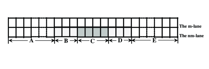
Figure 1:

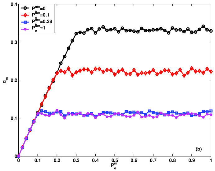
Figure 2:

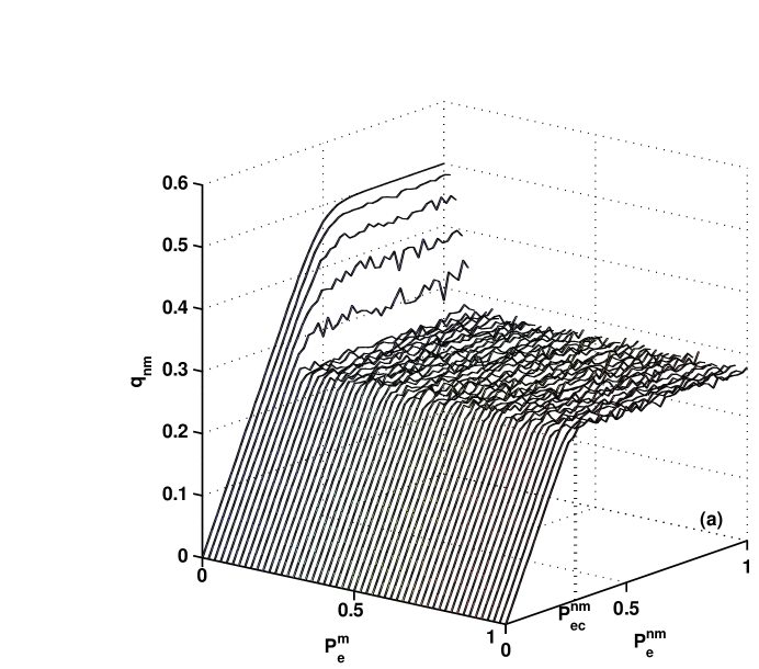
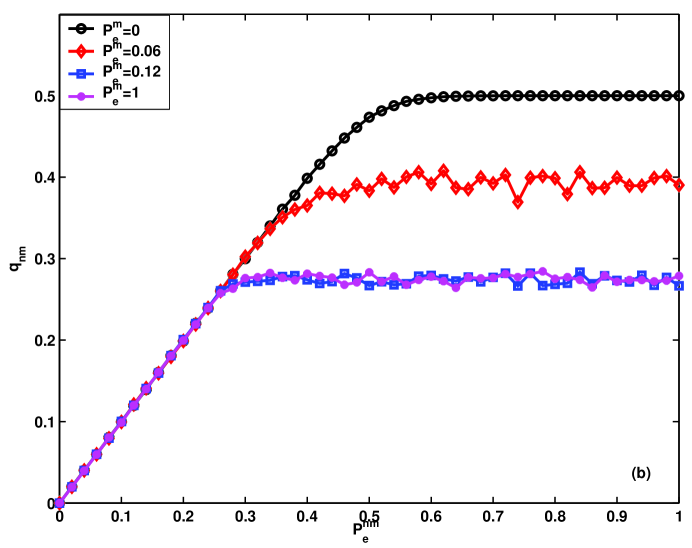
Figure 3:

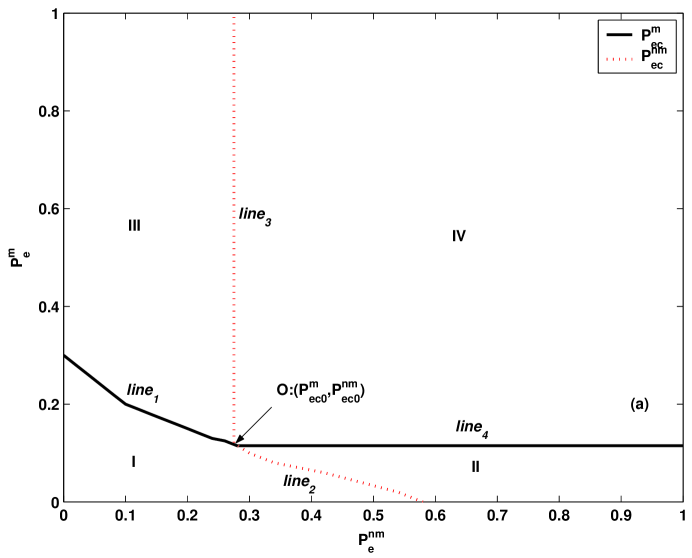
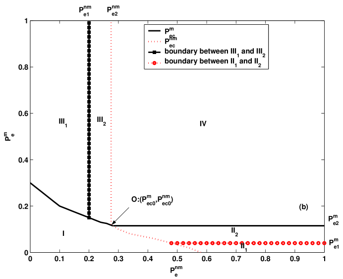
Figure 4:

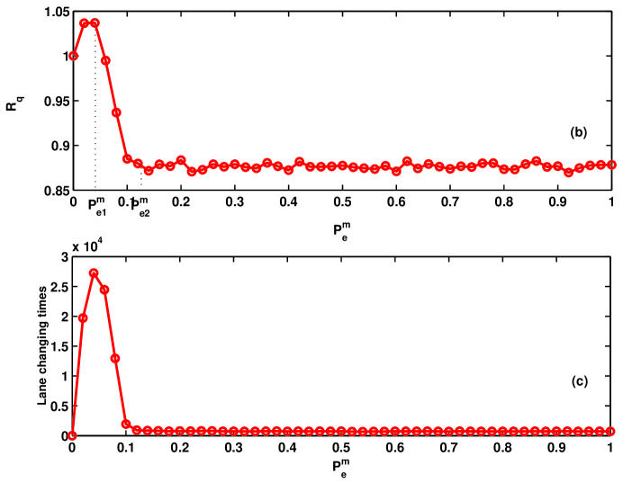
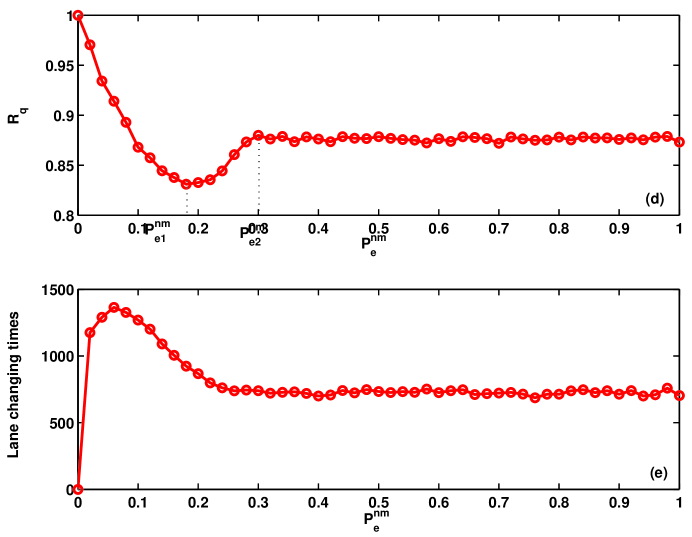
Figure 5: