[labelstyle=]
On the skein exact squence for knot Floer homology
Abstract.
The aim of this paper is to study the skein exact sequence for knot Floer homology. We prove precise graded version of this sequence, and also one using . Moreover, a complete argument is also given purely within the realm of grid diagrams.
1. Introduction
Knot Floer homology is an invariant for knots in defined using Heegaard diagrams and holomorphic disks [9], [12]. This invariant can be used to construct a bigraded group , endowed with an Alexander and a Maslov grading, has as its Euler characteristic the Alexander polynomial of the knot. Another variant gives a bigraded Abelian group , which is a module over the polynomial ring , and whose specialization (in a suitable sense) to gives .
The traditional skein relation for the Alexander polynomial translates into this context into a long exact sequence which relates of a knot with a distinguished positive crossing , the knot Floer homology of the oriented resolution of that crossing (which is a link), and also the knot Floer homology of the knot obtained by changing the distinguished positive crossing in to a negative crossing, see Figure 1. The first version of this exact triangle appeared in [9], where the term involving is defined using a suitable generalization of knot Floer homology to an invariant for oriented links, which we denote by .

Link Floer homology is given a more general definition in [8], as a multi-graded theory whose Euler characteristic is the multi-variable Alexander polynomial. Algebraically, the invariant is a multi-graded theory which is the homology of a chain complex over , where the formal variables are in one-to-one correspondence with the components of the link. The invariant appearing in the earlier skein exact sequence is the homology group gotten by setting all the , and adding up all of the “Alexander gradings”.
In [5], link Floer homology is given a purely combinatorial calculation via “grid diagrams”. This thread is pursued further in [6], where the basics of the theory are developed from a purely combinatorial point of view.
The aim of the present paper is to give a different proof of the skein exact sequence for knot Floer homology. The advantages of this proof is that it generalizes to the case of , and also we can give more precise grading information about the maps. Moreover, this perspective can be applied readily to give another (quite similar) proof which works purely within the context of grid diagrams. Aside from an aesthetic benefit, this also gives a direct combinatorial way to calculate the maps appearing in the skein exact sequence.
Theorem 1.1.
Let , , and be three links, which differ at a single crossing as indicated by the notation. Then, if the two strands meeting at the distinguished crossing in belong to the same component, so that in the oriented resolution the two strands corresponding to two distinct components and of , then there are long exact sequences
If they belong to different components, we have a long exact sequence
where here is the bigraded module
and is the bigraded module
The reader is warned: there are two natural conventions on Maslov grading, one which takes half-integral values (cf. [9]), and the other which always takes integral values (cf. [8]). In the above statement, we have adopted the latter convention.
A version of Theorem 1.1 appears in [9], except that the map defined there is not known to preserve Maslov gradings. This renders that version of the skein exact sequence somewhat cumbersome to use. It is interesting to note that the the module appears in for quite different reasons in the two approaches.
Two slightly different proofs of Theorem 1.1 are given. The first uses pseudo-holomorphic disks. The second is a combinatorial proof involving grid diagrams. This proof is slightly more awkward, as one cannot use a fixed grid diagram for all three knots; and of course, it is slightly less awkward in that it is a purely combinatorial argument, and the maps can be defined by explicit counts of polygons. Both proofs can be seen as a double iteration of the skein relating involving singular knots from [11], defined using Floer homology for singular knots from [7]. We have however chosen to give a more self-contained proof of Theorem 1.1 making no explicit reference to Floer homology for singular links; but our proof here is very similar in spirit to the proof of the skein sequence involving singular links, [11, Theorem LABEL:Resolutions:thm:SkeinExactSequenceIntro].
It is possible that the map defined here differs from the one used in [9]. It also seems different from the one used in [1]. In the next section, we briefly recall knot Floer homology, and set up our notation. In Section 3, we state and prove a theorem which specializes readily to Theorem 1.1.
1.1. Acknowledgements
We wish to thank Benjamin Audoux, Étienne Gallais, Matt Hedden, Ciprian Manolescu, and Dylan Thurston for interesting discussions.
2. Floer homology of knots and links
Knot Floer homology is a bigraded Abelian group associated to a knot in , cf. [9], [12]. We will briefly sketch this construction, and refer the reader to the above sources for more details.
Let be a surface of genus , let be a collection of pairwise disjoint, embedded closed curves in which span a -dimensional subspace of . This specifies a handlebody with boundary . Moreover, divides into components, which we label
Fix another such collection of curves , giving another handlebody . Write
Let be the three-manifold specified by the Heegaard decomposition specified by the handlebodies and . Choose collections of disjoint points and , which are distributed so that each region and contains exactly one of the points in and also exactly one of the points in . We can use the points and to construct an oriented, embedded one-manifold in by the following procedure. Let be an arc connecting the point in with the point in , and let be its pushoff into i.e. the endpoints of coincide with those of (and lie on ), whereas its interior is an arc in the interior of . The arc is endowed with an orientation, as a path from an element of to an element of . Similarly, let be an arc connecting to , and be its pushoff into . Putting together the and , we obtain an oriented link in .
Definition 2.1.
The data is called a pointed Heegaard diagram compatible with the oriented link .
An oriented link in a closed three-manifold always admits a compatible pointed Heegaard diagram. In this article, we will restrict attention to the case where the ambient three-manifold is .
Consider now the -fold symmetric product of the surface , . This space is equipped with a pair of tori
| and |
Knot Floer homology is defined using a suitable variant of Lagrangian Floer homology for this pair of subsets.
Specifically, let denote the set of intersection points . Let be the free module over generated by elements of , where here the are indeterminates.
To construct bigradings, consider functions
| and |
defined as follows. Given , let
where is any Whitney disk from to , and resp. is the algebraic intersection number of with the submanifold resp. . Also, let
where denotes the Maslov index of ; see [4] for an explicit formula in terms of data on the Heegaard diagram. Both and are independent of the choice of in their definition. There are functions and both of which are uniquely specified to overall translation by the formulas
| (1) | and |
The additive indeterminacy in and can be removed, as we explain at the end of the present subsection.
Let be the free module over generated by . This module inherits a bigrading from the functions and above, with the additional convention that multiplication by drops the Maslov grading by two, and the Alexander grading by one.
We define the differential
by the formula:
| (2) |
Here, denotes the moduli space of pseudo-holomorphic disks representing the homotopy class , divided out by the action of . The signed count is associated to an orientation system , which counts boundary degenerations with boundary entirely inside with multiplicity and those with boundary entirely inside with multiplicity . When is a knot, it it is sometimes convenient to consider instead the complex . The homology groups and are knot invariants [9], [12], see also [8], [5] for the case of multiple basepoints, and also [6] for a further discussion of signs. The bigradings on the complex induce bigradings on the homology
| and |
For an component link, we consider as a module over , where there is one variable corresponding to each component of . In this case, it is natural to consider , and their associated bigraded homology modules
| and |
In fact, was first defined in [9] using a slightly different construction, but the equivalence of the two constructions was established in [8, Theorem LABEL:Links:thm:IdentifyWithLinkHomology]. (In fact, in [8], a more general multi-graded theory is defined, with one Alexander grading for each component of the link. The present Alexander grading can be thought of as the sum of these Alexander gradings. We will have no need for this more general construction in the present paper.)
We have defined the bigradings only up to additive constants. This indeterminacy can be removed with the following conventions. Dropping the condition that all the in the differential for , we obtain another chain complex which retains its Maslov grading, and whose homology is isomorphic to (cf. [8, Theorem LABEL:Links:thm:InvarianceHFm]).
Similarly, the Alexander grading can be characterized as follows. If we consider the complex . This complex retains a -grading by , and its homology is isomorphic to as a relatively graded Abelian group. We fix the additive constant in the -grading by the requirement that
This in turn pins down that additive indeterminacy of .
2.1. Grid diagrams
Knot Floer homology has a combinatorial description for Heegaard diagrams associated to grid presentations according to [5], cf. also [6], [13].
A grid diagram is a Heegaard diagram for a knot, where the Heegaard surface is a torus, and all the (and the ) are parallel, homologically non-trivial circles. We draw the as horizontal, and the as vertical. The only non-trivial contributions in the differential are given by rectangles (and each such rectangles counts with a sign and also a product of variables associated to the the squares marked inside the rectangle). See [6] for a development of this complex which is logically independent of holomorphic curve techniques, including a proof of knot invariance.
More precisely, if denote the horizontal circles and are the vertical ones, our generating set consists of permutations , which we think of as -tuples of intersection points , . There are four embedded rectangles in the torus whose boundary consists of two segments within the and two segments with in the , and whose four corners are points from and . Two of these rectangles are oriented so that their oriented boundary meets the in a pair of arcs going from points in to points in . We say that those are the two rectangles from to , and we let denote this set of rectangles. If has the property that its interior contains none of the points from or , then we say is an empty rectangle.
In [6], we verify the existence of a map whith the following properties:
-
•
if are generators and , and , , then
-
•
if , are a pair of rectangles whose union forms a vertical annulus, then
-
•
if , are a pair of rectangles whose union forms a horizontal annulus, then
The chain complex associated to a grid diagram is freely generated by over , with differential given by
As in [5], this is a special case of the knot Floer homology chain complex considered earlier.
3. Proofs of the skein sequence
Theorem 1.1 follows from the following more general result, Theorem 3.1, which we state after introducing a few preliminaries.
Let be a positive crossing, and label its two outgoing edges by and , and its two in-coming ones by and , so that and are connected by the crossing, and and are connected in the resolution.
Recall that is an endomorphism of the chain complex , which drops Alexander grading by one and Maslov grading by two. Thus, we can form its mapping cone, which is a bigraded chain complex defined as follows. Letting denote the summand of in Alexander grading and Maslov grading , , endowed with the differential
This is quasi-isomorphic to the complex .
Theorem 3.1.
Let be a knot or link with a distinguished positive crossing, and let and be variables corresponding to the two out-going edges. There is a chain map whose mapping cone is quasi-isomorphic to the mapping cone of the chain map
In the case where both strands at belong to the same component of the knot, the quasi-isomorphism respects the bigrading, while in the case where the strands belong to different components, .
We will give two proofs of the above theorem. But first, we show that it implies Theorem 3.1.
Proof. [Theorem 3.1 Theorem 1.1] Suppose that is connected. In this case, skein exact sequence for follows immediately from Theorem 3.1, and the long exact sequence associated to a mapping cone. Consider next the case of . Then, we have that
Specializing our exact triangle to , we obtain a long exact sequence connecting connect , , and . Since the variables and correspond to basepoints and correspond to two different components of , we can identify the latter homology group with as desired.
Suppose that consists of two components both of which project to the distinguished crossing. This time, we have
Specializing our exact triangle to , we connect , , and the homology of the mapping cone of on . In , since and belong to the same strand, multiplication by is homotopic to multiplication to (this follows from general properties of stabilization, cf. [8, Section LABEL:Links:subsec:SimpleStabilizations], [5, Proposition LABEL:MOS:prop:ExtraBasepoints], see also [6, Lemma LABEL:lemma:ChainHomotopiesZ] for a proof using grid diagrams). Thus, the mapping cone of on is quasi-isomorphic to the tensor product of with . Similarly, for , we have a triangle connecting , and . Again, since and correspond to the same component, is null-homotopic, so the latter complex is quasi-isomorphic to .
Grading shifts are straightforward to verify (see the first proof of Theorem 3.1 for more discussion on this).
The more general case where consists of more components follows from the same reasoning as above, but a little bit of extra notation.
We give two proofs of Theorem 3.1. The first is a pseudo-holomorphic curves proof, and the second combinatorial proof uses grid diagrams.
3.1. Holomorphic curves proof
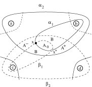
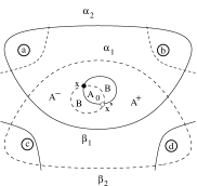
Our first proof of Theorem 3.1 involves inspecting a suitable Heegaard diagram, pictured in Figure 2. (This is also the route towards proving the exact triangle for singular knots appearing in [11].)
Draw a Heegaard diagram near a crossing as shown in Figure 2. In that picture, we have distinguished circles and which meet in two points and . This diagram is marked with , and , where . Alternatively, if we leave in and , and use , we obtain a Heegaard diagram for . Leaving in and , and using , we obtain a Heegaard diagram for the knot with positive crossing . Finally, using as the union of and the two regions marked by , we obtain a Heegaard diagram for the smoothing of the crossing.
Note that there are four circles of type in the picture, two of which correspond to the outgoing edges and , and two of which corresponding to the incoming ones and .
Clearly, has a subcomplex consisting of configurations which contain the intersection point , and a quotient complex . Thus, can be thought of as the mapping cone of the map
gotten by counting Maslov index one holomorphic disks representatives of homology classes which contain exactly one of the regions marked by (and hence neither of the regions marked or ), and also none of the ones marked by the other ,; i.e.
The understanding here is that the complex (and also ) is endowed with an induced differential which counts holomorphic disks which do not cross any of the four basepoints , , , or . (There are, however, no constraints placed on the multiplicity in . It is not difficult to see, though, that the other constraints imply that can be crossed at most once, and only for the differential within ).
Moreover, has as a subcomplex, with quotient , and hence, it can be thought of as the mapping cone of the map
defined by counting flowlines which contain exactly one of the regions marked by or .
Similarly, there is a subcomplex of consisting of configurations which contain the intersection point . This has a quotient complex we denote by . Moreover, has a subcomplex isomorphic to and quotient complex isomorphic to . Thus, we can think of as a mapping cone of
gotten by counting flowlines which contain exactly one of the regions marked by , and neither of the regions marked by or . Similarly, we can think of as the mapping cone of
which counts flowlines through exactly one of or , and neither of the regions marked by .
There is an obvious isomorphism , gotten by replacing the component by . It is straightforward to verify that this is a chain map.
Consider the maps
| and |
where here is defined by counting holomorphic disks modulo translation in Maslov index one homotopy classes with , and satisfying the addition conditions that
| and |
similarly, define to count holomorphic disks in homotopy classes with
| and |
Lemma 3.2.
The following relations hold:
where and denote the differentials on and respectively, and the right-hand-side represents multiplication by the scalar (thought of as an endomorphism of or ). Informally, one can think of as furnishing a homotopy between and multiplication by ; and as furnishing a homotopy between and multiplication by .
Proof. This is analogous to the proof (which uses Gromov’s compactness theorem [3]) that in Floer homology (cf. [10], and [2] for a general discussion).
We consider the case of . Look at ends of one-dimensional moduli spaces connecting to for homotopy classes which satisfy and . These ends consist either of broken flowlines, or boundary degenerations. Broken flowlines are parameterized by pairs of homotopy classes of Maslov index one homotopy classes , for some . These can be partitioned into four cases:
-
•
and
-
•
and
-
•
and
-
•
and .
The first types are counted in , the second by , the third , and the fourth in .
The contributing boundary degenerations in the ends of this moduli space consist of Maslov index two holomorphic disks with boundary in or , and which contain both one point from and one in . There are four of these, one of which contains each of , , , or respectively (compare [11, Lemma LABEL:Resolutions:lemma:CalcComposite]).
We form now the chain complex , given by the diagram:
where . In fact, the above diagram can be used to form a chain complex thanks to Lemma 3.2. We denote this complex by .
Clearly, the above complex has a subcomplex, corresponding to the rightmost column, which is the mapping cone of , which in turn is identified with , while its quotient complex is the mapping cone of , which in turn is identified with .
Moreover, the bottom row is a subcomplex in turn is identified with ; its quotient complex is the top row which also is identified with .
Lemma 3.3.
Under the identification of both rows of with , the vertical map is homotopic via to multiplication by .
Proof. This follows along the lines of Lemma 3.2. We can think of as the map gotten by counting holomorphic disks which cross . Now the sum of vertical maps is induced by . Moreover, the map induces a homotopy of this map with the count of all boundary degenerations containing both and . This latter map is readily seen to correspond to multiplication by .
Proof. [of Theorem 3.1] As we have seen, the complex is simultaneously identified with the mapping cone of a map , and the mapping cone of a map which is chain homotopic to multiplication by , which in turn is quasi-isomorphic to , as desired.
We turn our attention to gradings. Configurations and inherit Maslov and Alexander gradings from either or ; similarly, configurations in or inherit Maslov and Alexander gradings from either or . We assert that all the induced Maslov gradings coincide. This is clear since the Maslov grading of a given generator is independent of the placement of points of type , depending only on the placement of the (which coincide for all three links).
Consider next the -gradings. After setting all , we can isotope across the to obtain the same diagram for and . Thus the -gradings of the two diagrams agree. Thus, it follows that (absolute) -gradings for and coincide for all generators.
Now consider the horizontal connecting homomorphism . This map clearly preserves both Alexander and Maslov gradings. For example, we can view the restriction of to the subcomplex . The component of the connecting homomorphism is gotten by counting holomorphic disks which cross exactly one of or , a map which simultaneously drops and -degree by one, post-composed by the inverse of , which simultaneously raises both of these degrees by one.
Using the bigrading grading on for which the projection map respects bigradings so that , we then have a bigraded identification
where all identifications are made using the diagram for . In fact, under the bigraded isomorphism with the mapping cone of , we have that
where once again all bigradings are induced from .
Suppose now that the two strands in belong to the same component. In this case, we claim and induce the same the bigrading on . To see this, observe that in the complex, a generator for , when thought of as an element of has grading one greater than the same same element thought of as a generator for for . Thus, we have a bigraded identification
Similarly, if the two strands in belong to different components, then the Alexander grading of a generator from thought of as represented in is one less than its Alexander grading thought of as a represented in ; hence we have that
3.2. Proof using grid diagrams
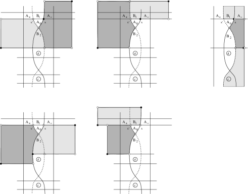
A disadvantage of the grid diagrams proof is that there is no grid diagram which represents all three knots , , and ; instead, one has to move the grid diagram, as pictured in Figure 4. By way of explanation, we have the Heeegaard torus, equipped with , , and horizontal circles . We have two possible sets of vertical circles and , which differ only in the choice of the first circle (i.e. for ), and . We call the two grid diagrams and . The circles and meet in two points, one of which is labelled as shown in the picture. Note that there is a small triangle bounded by an arc in an -circle, an arc in , and an arc in , which contains in its interior, and whose three vertices are (on ), (on ) and .
In the present context, the complex is generated by generators which contain the intersection point , while is generated by generators which contain the intersection point . These are made into complexes by counting rectangles which are disjoint from and . There are also complexes and defined using the complementary sets of generators. As before, we have maps
The first two of these maps is defined by by counting rectangles in : the first counts rectangles which contain one of or , the second counts rectangles which contain one of or . The second two use rectangles in the diagram , the first counts rectangles containing or , and the second counts rectangles containing or . There is also an identification gotten by moving the intersection point to .

Lemma 3.4.
We have the following relations:
Proof. This is essentially a repetition of Lemma 3.2, except, of course, that for grid diagrams, arguments like Gromov’s compactness theorem can be formulated in purely combinatorial terms (cf. [6, Proposition LABEL:MOST:prop:DSquaredZero]).
We start with the first equation. Observe that the sum of maps counts polgons obtained by juxtaposing two rectangles, one of which contains or , and the other contains or . These polygons cancel in pairs, except for those annuli of length or width equal to one, which contain both or and or , of which there are four, contributing . In principle, there might be alternative decompositions consisting of a rectangle without either , , , or (and the other must have one of each pair). But there are no such alternative decompositions with initial point at . In a similar vein, it is straightforward to see that annihilates .
The second relation follows similarly.
According to Lemma 3.4, the following diagram represents a chain complex:
| (3) |
Let be the chain complex for the resolution using in Figure 4, and be the chain complex for using . An explicit chain homtopy equivalence
is constructed in [6, Subsection LABEL:MOST:subsec:Commutation]. This map is defined by counting pentagons. More precisely, given and , we let denote the space of embedded pentagons with the following properties. This space is empty unless and coincide at points. An element of is an embedded disk in , whose boundary consists of five arcs, each contained in horizontal or vertical circles. Moreover, under the orientation induced on the boundary of , we start at the -component of , traverse the arc of a horizontal circle, meet its corresponding component of , proceed to an arc of a vertical circle, meet the corresponding component of , continue through another horizontal circle, meet the component of contained in , proceed to an arc in until we meet the intersection point , and finally, traverse an arc in until we arrive back at the initial component of . Finally, all the angles here are required to be less than straight angles. The space of empty pentagons with , is denoted .
Given , define
It is elementary to see that the above map induces a chain homotopy equivalence [6, Proposition LABEL:MOST:prop:Commute].
Lemma 3.5.
Under the natural identification of the two rows in the above complex with chain complexes for , the two vertical maps add up to multiplication by .
Proof. Let be the chain complex for appearing in the top row of Equation (3), and let be the complex for appearing in the bottom row. Thus, belongs to the grid diagram , while belongs to the grid diagram . The sum of the two vertical maps can be viewed as a chain map , where
We have a map defined by counting pentagons, as above.
We will find it convenient to extend the maps and earlier to maps
| and |
gotten by counting rectangles which contain both and . Similarly, we have a map and defined by counting rectangles which contain .
We claim that
| (4) |
This is seen as follows. The composite is a count of polygons, which are gotten by juxtaposing an empty rectangle starting at an intersection point from , followed by an empty pentagon. By filling in the small triangle containing , we obtain a one-to-one correspondence between these polgons, and polygons obtained in the following way:
-
(1)
juxtapositions of two rectangles, the first of which contains and the second of which contains
-
(2)
juxtapositions of rectangles, the first of which is empty, and the second of which contains both and
-
(3)
the column in through both and and .
The first term contibutes . Decomposing the polygon in an alternative way, we see that the sum of the second two terms contributes . (Note that the column in through and contributes , which is the same as the contribution the column in of the column through and .)
Similarly, we claim that
| (5) |
This follows more directly than Equation (4). Filling in the small triangle containing , we obtain a one-to-one correspondence between the polgons counted on both sides.
Adding Equations (4) and (5), we conclude that . The same arguments from Lemma 3.4 show that the following relation holds:
i.e. is homotopic to multiplication by , as desired.
Proof. [Grid diagram proof of Theorem 3.1.] The proof follows from inspecting the complex from Equation (3), which we refer to now as . Again, the two vertical columns correspond to and respectively, and so the horizontal maps add up to give the stated map . Moreover, according to Lemma 3.5, is quasi-isomorphic to the mapping cone of
Gradings can be traced through exactly as in the earlier proof.
References
- [1] B. Audoux. Heegaard-Floer homology for singular links. arXiv:0705.2377.
- [2] K. Fukaya, Y-G. Oh, K. Ono, and H. Ohta. Lagrangian intersection Floer theory—anomaly and obstruction. Kyoto University, 2000.
- [3] M. Gromov. Pseudo holomorphic curves in symplectic manifolds. Inventiones mathematicae, 82:307–347, 1985.
- [4] R. Lipshitz. A cylindrical reformulation of Heegaard Floer homology. math.SG/0502404, 2005.
- [5] C. Manolescu, P. S. Ozsváth, and S. Sarkar. A combinatorial description of knot Floer homology. math.GT/0607691.
- [6] C. Manolescu, P. S. Ozsváth, Z. Szabó, and D. P. Thurston. On combinatorial link Floer homology. math.GT/0610559.
- [7] P. S. Ozsváth, A. Stipsicz, and Z. Szabó. Floer homology and singular knots. arXiv:0705.2661.
- [8] P. S. Ozsváth and Z. Szabó. Holomorphic disks and link invariants. math.GT/0512286.
- [9] P. S. Ozsváth and Z. Szabó. Holomorphic disks and knot invariants. Adv. Math., 186(1):58–116, 2004.
- [10] P. S. Ozsváth and Z. Szabó. Holomorphic disks and topological invariants for closed three-manifolds. Ann. of Math. (2), 159(3):1027–1158, 2004.
- [11] P. S. Ozsváth and Z. Szabó. A cube of resolutions for knot Floer homology. arXiv:0705.3852, 2007.
- [12] J. A. Rasmussen. Floer homology and knot complements. PhD thesis, Harvard University, 2003.
- [13] S. Sarkar and J. Wang. A combinatorial description of some Heegaard Floer homologies. math.GT/0607777.