A Renormalization Group For Treating 2D Coupled Arrays of Continuum 1D Systems

Abstract

We study the spectrum of two dimensional coupled arrays of continuum one-dimensional systems by wedding a density matrix renormalization group procedure to a renormalization group improved truncated spectrum approach. To illustrate the approach we study the spectrum of large arrays of coupled quantum Ising chains. We demonstrate explicitly that the method can treat the various regimes of chains, in particular the three dimensional Ising ordering transition the chains undergo as a function of interchain coupling.

The density matrix renormalization group (DMRG) white is one of the primary theoretical tools for the quantitative description of low dimensional lattice models. For a wide range of one dimensional (1D) lattice models, DMRG can characterize the model’s spectrum and correlation functions kuhn . While there have been notable recent advancements moukouri ; white2 , its use on 2D lattice models is more circumscribed hallberg .

There exist several strategies to apply DMRG to 2D models. In the first, the 2D lattice is reduced to a 1D lattice with long range interactions noack . A second approach sees short chains treated as individual lattice sites, allowing the 1D DMRG algorithm to be applied to a model with short ranged interactions directly jongh . In a more sophisticated variant of this methodology, the DMRG is applied in a two stage process moukouri . The 2D system is first divided into a set of coupled 1D chains and the DMRG is used to determine a low energy reduction thereof. For the second stage, the reduced chains, coupled together and treated as individual lattice sites in a 1D lattice, are analyzed again using DMRG. In a final approach, the 1D matrix product states underlying the DMRG algorithm ostlund are replaced by a higher dimensional generalization, projected entangled pair states ver .

In this letter we present a distinct approach to applying DMRG to 2D models. This approach trades upon a description of a 2D system as a mixture of continuum and discrete degrees of freedom. In particular, we approach 2D systems as coupled arrays of continuum 1D chains with truncated Hilbert spaces. This methodology offers several distinct advantages. It allows us to treat any 2D strongly correlated model provided it can be conceived as composed of continuum 1D subunits. Furthermore, the approach affords superior finite size scaling. As a function of the length, $R$, of the composite 1D systems, finite size corrections behave exponentially. This implies that we can access, at the very least, the infinite volume limit in the dimension parallel to the chains. Finally, the truncation of the underlying 1D Hilbert space dramatically lessens the numerical burden of the DMRG algorithm, while providing a natural means to perform a Wilsonian renormalization group (RG) improvement of any resulting answer first .

The specific type of system that we propose to study takes the form,

$$H=\sum_{i}H^{1D}_{i}+J\sum_{<ij>}{\cal O}_{i}{\cal O}_{j}.$$ (1)

The 1D continuum subunits of the array are governed by $H^{1D}_{i}$ which we insist must be either gapless (and so governed by a conformal field theory) or gapped but integrable note . Thus this method can study, for example, arrays of Luttinger liquids and a wide range of coupled 1D Mott insulators. The subunits are coupled together via the nearest neighbour coupling $J{\cal O}_{i}{\cal O}_{j}$, where ${\cal O}_{i}$ is an operator defined along the i-th continuum chain. This coupling should be relevant but can be of arbitrary strength.

The analysis of the arrays proceeds in two conceptual steps. In the first step we follow Zamolodchikov’s pioneering numerical analysis of perturbed gapless 1D continuum theories zamo , an approach termed the truncated spectrum approach (TSA). We thus place the 1D chains on a ring of circumference, $R$. Unlike DMRG applied to pure lattice models, periodic boundary conditions along the chains can be employed without issue. By working at finite $R$, we discretize the 1D spectrum. This permits the states in the chains’ spectrum to be ordered in energy, i.e. $|1\rangle,|2\rangle,\ldots$, and then truncated at some finite cutoff, $E_{c}$, leaving us with a finite number of states in the theory. With these alterations we nonetheless remain in an excellent position to obtain information regarding the full theory in infinite volume. In Ref. zamo , a critical Ising chain in a magnetic field was studied. Choosing $E_{c}$ so that a mere $39$ states were kept, infinite volume results were reproduced within an error of $2\%$ (via diagonalization of a $39\times 39$ matrix). It was this finding of excellent results at little numerical cost that motivated us to apply the TSA to more complicated situations first , including, as here, arrays of 1D chains.

A part of the TSA’s success is predicated on embedding non-perturbative information into the initial computation. In the context at hand this means that given any two states, $|k\rangle,|l\rangle$, we can exactly compute matrix elements of the form $\langle k|{\cal O}_{i}|l\rangle$ by virtue of $H^{1D}_{i}$ either being conformal or integrable. We stress that computation of such matrix elements is always a practical possibility either by exploiting the algebraic structures inherent in a conformal field theory or the form factor bootstrap approach in the case of a integrable field theory ffprog .

Having prepared the chains by truncating their finite volume spectrum, we proceed to the actual analysis of coupled arrays. We perform the analysis using the finite volume DMRG algorithm. Here each chain with truncated spectrum is treated as if a single site. We however adapt the DMRG algorithm to take into account that we are working with a truncated spectrum. This algorithm is outlined in Table 1.

Table 1: Finite system DMRG algorithm adapted to the presence of a truncated spectrum.

1.	Form initial Hamiltonian, $H_{m-1}$, (and any other needed
	operators, ${\cal O}_{m-1}$) of system block, $B_{m-1}$, of m-1 chains.
2.	Form Hamiltonian of superblock, $B_{m-1}\bullet\bullet B_{m-1}$, of 2m
	chains, only keeping states whose energy, governed by
	$H_{m-1}\otimes H^{1D}\otimes H^{1D}\otimes H_{m-1}$, i.e. coupling between
	the blocks is absent, is less than $E_{c}$.
3.	Find low-energy target state(s) of superblock. Form
	reduced density matrix of m-chain block, $\rho_{m}$.
4.	Diagonalize $\rho_{m}$, keeping sufficient eigenstates to
	obtain a truncation error of less than $\epsilon_{c}$.
5.	Recast $H_{m}$ and ${\cal O}_{m}$ in basis of kept eigenstates of $\rho_{m}$,
	obtaining $\bar{H}_{m}$ and $\bar{{\cal O}}_{m}$.
6.	Diagonalize $\bar{H}_{m}$, obtaining $\bar{H}^{*}_{m}$. Rewrite $\bar{{\cal O}}_{m}$ in terms of
	eigenstates of $\bar{H}^{*}_{m}$.
7.	Form new superblock, $B_{m}\bullet\bullet B_{m}$, of length 2m+2.
	As determined by ${\bar{H}}^{*}_{m}\otimes H^{1D}\otimes H^{1D}\otimes{\bar{H}}^{*}_{m}$, only keep
	states whose energy is less than $E_{c}$.
8.	Repeat 3-7 with $m\rightarrow m+1$ until desired length of
	system is obtained.
9.	Perform finite volume sweeps until convergence.

Most steps of our finite system DMRG algorithm are unchanged from the standard algorithm white1 . One primary difference lies in the formation of the superblock Hilbert space and Hamiltonian (steps 2 and 7 in Table 1). Instead of keeping all states in the Hilbert space, we insist that the state have an energy less than the truncation energy, $E_{c}$, as governed by the Hamiltonian of the uncoupled blocks. Concomitantly in order to meaningfully associate an energy with an arbitrary state of a superblock, we must be able to assign an energy to the states of each block.

Figure 1: a) A sketch of an array of Ising chains, each of length R; b) a zero temperature phase diagram of the coupled chains showing both the ordered and disordered regions.

This mandates that at each iteration of the DMRG we must not only recast the block Hamiltonian, $H_{m}$, in terms of the kept eigenstates of the reduced density matrix, $\rho_{m}$ (step 5), obtaining $\bar{H}_{m}$, but we must diagonalize $\bar{H}_{m}$ (step 6). Working then with a basis of eigenstates of $\bar{H}_{m}$ allows us to associate a definite energy to the superblock states formed in the next step (step 7).

A notable operational feature of this DMRG is the relatively small number of states we need to keep from the diagonalization of the reduced density matrix in order to achieve a given truncation error. In the example of arrays of coupled quantum Ising chains that we consider below, the number of kept states needed to achieve truncation errors on the order of $5\times 10^{-5}$ ranges from $10-40$ deep in the ordered phase of the chains to $50-90$ near the critical value of the interchain coupling where the chains order.

The relatively small number of states needed to achieve a given accuracy mimics Zamolodchikov’s original finding that a relatively small number of states was needed to describe a critical Ising chain in a magnetic field. But it also reflects the presence of a truncated spectrum in our approach. As was shown in Ref. callan , the entanglement entropy that arises from dividing a 2D system into two behaves as the cutoff, $E_{c}$. As the entanglement entropy is one measure of whether a DMRG-like algorithm will be successful ver ; hallberg , we believe that our introduction of a cutoff into the problem is a key feature of our approach.

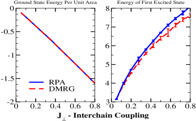
Figure 2: The ground state and first excited state energy of a 100 chain array as a function of interchain coupling obtained with both a random phase approximation (blue solid) and our DMRG methodology (red dashed). Here $\Delta=1$.

A second key but related feature that marks our use of the DMRG algorithm is the use of RG improvement. For sufficiently large truncation energies, $E_{c}$, the quantities of interest (whether it be the spectrum or some observable) satisfy a one-loop RG flow first :

$$\frac{d\Delta Q}{d\ln E_{c}}=-g\Delta Q.$$ (2)

Here $\Delta Q=Q(E_{c})-Q(E_{c}=\infty)$ is the deviation of some quantity as a function of the truncation energy from its value at $E_{c}=+\infty$. The function $g$ is a constant determinable from high energy perturbation theory and is related to the anomalous dimension of $Q$. When Q is an energy of some state, $g=1$. Knowledge of this flow allows us to run the DMRG algorithm at several different truncation energies and then extrapolate the resulting flow to $E_{c}=+\infty$, so removing any residual effect of our use of a finite value for $E_{c}$.

Coupled Ising Chains: To demonstrate this methodology we consider arrays of Ising chains (Fig. 1a) coupled via a nearest spin-spin perturbation:

$$H=\sum_{i}H^{1D~{}Ising}_{i}-J_{\perp}\sum_{<ij>}\sigma^{z}_{i}\sigma^{z}_{j},$$ (3)

where the summations are over the chains in the array. The lattice form of the 1D Ising model is

$$H^{1D~{}Ising}=-J\sum_{i}(\sigma^{z}_{i}\sigma^{z}_{i+1}+(1+g)\sigma^{x}_{i}).$$ (4)

Its continuum version is a Majorana fermion with gap, $\Delta=gJ$. We place the chain on a ring of circumference, $R$. The corresponding Hilbert space of the chain divides itself into two sectors, termed Neveu-Schwarz (NS) and Ramond (R). At T=0, the chain can be either ordered or disordered. In its disordered phase, $\Delta<0$, the NS/R sectors of the chain permit only even/odd numbers of free fermionic excitations. In the ordered phase, $\Delta>0$, the two sectors both permit only states with even numbers of fermions. The matrix elements of the spin operator, $\langle i|\sigma^{z}|j\rangle$, needed to carry out the DMRG procedure can be found in Ref. fonseca . These matrix elements are only non-vanishing if the states $|i\rangle$ and $|j\rangle$ lie in different sectors of the theory. Because we couple the chains together with nearest neighbour spin bilinears, i.e. $\sigma^{z}_{i}\sigma^{z}_{i+1}$, the Hilbert space of the full theory possesses two sectors. Any given state of the full theory has a tensor form $\otimes_{i}|k_{i}\rangle$ where $|k_{i}\rangle$ is a state on the i-th chain. These two sectors are distinguished by whether an even or odd number of the $|k_{i}\rangle$ lie in the NS sector (or equivalently, the R sector) of the individual chains. That the Hilbert space possess different sectors is a generic feature of continuum models when placed in finite volume and is not particular to the Ising chains at hand.

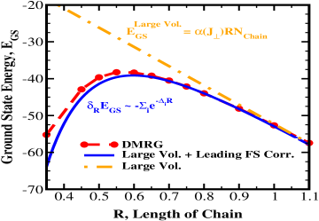
Figure 3: The behavior of the ground state energy as a function of chain length, $R$, for 100 chains. $J_{\perp}=0.275$. In blue we see the analytic prediction while in red we see the results of the DMRG.

We now submit the DMRG algorithm to a number of tests. The first test that we apply relates to the behaviour of the spectrum of the chains deep in their ordered phase ($\Delta>0$ – see the phase diagram in Figure 1b). In this region of the phase diagram, we expect a chain RPA analysis to be accurate carr and so provide a baseline of comparison for our DMRG results. The chain RPA analysis amounts to treating the model

$$H^{I.C.Array}_{RPA}=-J\sum_{i}(\sigma^{z}_{i}\sigma^{z}_{i+1}+(1+g)\sigma^{x}_{i}+h_{RPA}\sigma^{z}_{i}),$$ (5)

where $h^{RPA}$ is chosen in the standard self-consistent fashion carr . We analyze this model numerically using the truncated spectrum approach along the same lines as Ref. fonseca . However akin to the discussion surrounding Eqn. (2) and in Ref. first , we perform an RG improvement of our numerical results.

In Fig. 2 we plot the ground and first excited state energy of a 100-chain array as a function of the interchain coupling as computed by both the DMRG and the chain RPA analysis. In order to optimize numerical performance, we employ different chains lengths for different values of $J_{\perp}$. To obtain $R=\infty$ values for the gaps, $\Delta_{exc}$, of single excitations, we can use any finite value of $R$ provided that we satisfy $R\Delta_{exc}\gg 1$. Because finite $R$ corrections behave exponentially, $\delta_{R}\Delta_{exc}\sim e^{-R\Delta_{exc}}$, this constraint need only be satisfied loosely. In order to obtain a truncation error,$\epsilon_{c}$ of $1\times 10^{-4}$ we needed to keep at most 18 states. Decreasing the truncation error to $2.5\times 10^{-6}$ we needed to keep at most 34 states. Moreover by comparing our results with an analysis of 50 coupled chains, we know that any finite size error related to studying only a finite number of chains is extremely small. The only significant uncertainty comes from the RG improvement – applying Eqn. (2) – and is the source of the error bars in Fig. 2.

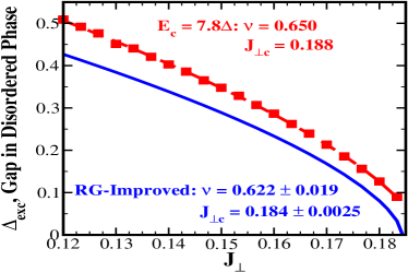
Figure 4: The behavior of the gap in the disordered phase as a function of $J_{\perp}$ for 60 coupled chains at $R=10\Delta$. In red we plot the gap as determined for the truncation energy $E_{c}=7.8\Delta$, while in blue we plot the RG-improved curve. For both, the values of $J_{\perp c}$ and $\nu$ are indicated.

We see from Fig. 2 that the ground state energy as determined by the DMRG agrees exceptionally well with the chain RPA analysis even for values of the interchain coupling on the same order as the gap. The DMRG values of the gap for the first excited state however see increasing deviations from the RPA values as the interchain coupling is increased. These results indicate that the truncated DMRG algorithm is operating as expected.

A more significant test of the algorithm is whether it predicts correctly the finite $R$ corrections. These corrections can be computed analytically, at least at leading order. According to Ref. zamo , they take the form

$$\delta_{R}E_{gs}=-\frac{1}{2\pi}\sum_{b}\sum_{k_{y}}\int dk_{x}e^{-R\epsilon_{b}(k_{y},k_{x})},$$ (6)

and can be thought of as arising from spontaneous emission of excitations from the vacuum. Here $\epsilon_{b}(k_{y},k_{x})$ is the dispersion of some band $b$ of excitations in the coupled chains. $\delta_{R}E_{gs}$ sees contributions from excitations with different (discrete) values of momenta, $k_{y}$, transverse to the chains as well as excitations with different (continuum) values of the momenta, $k_{x}$, parallel to the chains. While we cannot compute $\epsilon_{b}$ exactly, we can estimate it from the values of the excited states as measured by the DMRG together with an RPA analysis carr :

$$\epsilon_{b}(k_{y},k_{x})=(v_{Fx}^{2}k_{x}^{2}+\Delta_{b~{}exc}^{2}+2J_{\perp}Z_{o}(1-\cos(k_{y})))^{1/2}.$$ (7)

Here $\Delta_{b~{}exc}$ marks the lowest lying excitation in the band, while $Z_{o}$ is the square of a matrix element of the spin operator on a single chain, $Z_{o}=2\langle 0|\sigma_{i}^{z}(0)|\epsilon_{b}(k_{x}=0,k_{y}=0)\rangle^{2}$. The latter quantity is estimated from the same analysis used in computing the RPA energies of Fig. 1.

In Fig. 3 we plot $E_{gs}(R)$ for a particular value of interchain coupling ($J_{\perp}=0.275$) using the correction in Eqn. 6 by taking into account the two lowest energy bands in the theory (blue dashed line) vs. the direct DMRG computation (red line). We see that for all but the smallest values of $R$ – where our leading order analytic approximation breaks down – the DMRG and expected analytic values agree well. For a point of comparison, we also plot the extrapolation of the energy from large values of $R$, where $E_{gs}$ scales linearly with system volume, i.e. $E_{gs}(R)=\alpha(J_{\perp})RN_{chain}$ (straight dashed orange curve). For values of $R\sim\Delta_{b~{}exc}^{-1}$ the finite size corrections are exponentially suppressed, consistent with $\Delta_{b~{}exc}=5.1\Delta$ for $J_{\perp}=0.275$ (from Fig. 1).

The final test we put to the truncated DMRG algorithm is the chains’ ordering transition. Beginning with chains in their disordered state ($\Delta<0$) and coupling them together with increasing $J_{\perp}$, they eventually order. This transition is in the same universality class as the 3D Ising model. This implies that the gap, $\Delta_{exc}$, in the disordered phase should vanish as $\Delta_{exc}\sim(J_{\perp c}-J_{\perp})^{\nu}$ with $\nu=.630$ camp . From our DMRG analysis (see Fig. 4), we find after RG improvement, $J_{\perp c}=.184\pm.0025$, together with good agreement for the critical exponent, $\nu=.622\pm.019$. We see that RG improvement notably improves the results. Computing instead $J_{\perp c}$ and $\nu$ from the results obtained at the largest of the truncation energies employed ($E_{c}=7.8\Delta$), we obtain $J_{c}=.1880$ and $\nu=0.650$.

This DMRG approach to 2D arrays of continuum systems has a number of potentially valuable variations. We first note that we have managed to treat 2D arrays using essentially a 1D DMRG algorithm. Ref. moukouri has demonstrated that the DMRG algorithm, if used in a two stage process, can treat systems of one higher dimension. This implies that it may well be possible to study 3D arrays using our approach. We also note that the algorithm we have outlined in this letter may see substantial improvement if wedded to a numerical renormalization group (NRG) à la Wilson wilson . At each DMRG iteration, one could perform a NRG akin to that described in Ref. first to dramatically increase the truncation energy being employed and so (hopefully) dramatically improve the results of the procedure.

To summarize, we have demonstrated that the 1D DMRG algorithm can be directly applied to 2D arrays of 1D continuum systems. In particular we have shown this algorithm can describe the behavior of large arrays of quantum Ising chains both in their ordered phase and in the vicinity of their order-disorder transition. We expect that this procedure will produce quantitatively accurate results on a wide variety of 2D systems in their infinite volume limit.

RMK and YA acknowledge support from the US DOE (DE-AC02-98 CH 10886) together with useful discussions with A. Tsvelik.

References

- (1) S. R. White, Phys. Rev. Lett. 69, 2863 (1992).
- (2) T. D. Kühner and S.R. White, Phys. Rev. B 60, 335 (1992).
- (3) S. Moukouri, Phys. Rev. B 70, 014403 (2004).
- (4) S. White and A. Chernyshev, arXiv:0705.2746.
- (5) K. Hallberg, Adv. Phys. 55, 447 (2006); cond-mat/0609039.
- (6) R. Noack and S. Manmana, AIP Conf. Proc. 789, 93 (2005); cond-mat/0510321.
- (7) M. de Jongh et al., Phys. Rev. B 57, 8494 (1998).
- (8) S. Ostlund and S. Rommer, Phys. Rev. Lett. 75, 3537 (1995).
- (9) F. Verstraete and J. Cirac, cond-mat/0407066.
- (10) R. M. Konik and Y. Adamov, Phys. Rev. Lett. 98, 147205 (2007).
- (11) The requirement of integrability for gapped systems can be relaxed but at additional numerical cost.
- (12) V. P. Yurov and Al. B. Zamolodchikov, Int. J. Mod. Phys A 6, 4557 (1991).
- (13) F. Smirnov, “Form Factors in Completely Integrable Models of Quantum Field Theory”, World Scientific, Singapore (1992).
- (14) S. R. White, Phys. Rev. B 48 10345 (1993).
- (15) C. Callan and F. Wilczek, Phys. Lett. B 333, 55 (1994).
- (16) P. Fonseca and A. Zamolodchikov, J. Stat. Phys. 110, 527 (2003).
- (17) K. Wilson, Rev. Mod. Phys. 47, 773 (1975).
- (18) S. T. Carr and A. M. Tsvelik, Phys. Rev. Lett. 90, 177206 (2007).
- (19) M. Campostrin et al., Phys. Rev. E 60, 3526 (1999).