QCD dynamics in a constant chromomagnetic field

Abstract:

We investigate the phase transition in full QCD with two flavors of staggered fermions in presence of a constant abelian chromomagnetic field. We find that the critical temperature depends on the strength of the chromomagnetic field and that the deconfined phase extends to very low temperatures for strong enough fields. As in the case of zero external field, a single transition is detected, within statistical uncertainties, where both deconfinement and chiral symmetry restoration take place. We also find that the chiral condensate increases with the strength of the chromomagnetic field.

1 Introduction

In previous studies [1, 2] on the vacuum dynamics of pure non-abelian gauge theories we found that the deconfinement temperature depends on the strength of an external abelian chromomagnetic field. In particular we ascertained that the deconfinement temperature decreases when the strength of the applied field is increased and eventually goes to zero. It is not difficult to see here an analogy with the reversible Meissner effect in the case of ordinary superconductors (where the system goes to normal even at zero temperature if the magnetic field is strong enough) and therefore we referred to it as ”vacuum color Meissner effect”. We have also verified that the same effect is not present in the case of abelian gauge theories, so that it seems to be directly linked to the non-abelian nature of the gauge group.

The dependence of the deconfinement temperature on applied external fields is surely linked to the dynamics underlying color confinement, therefore in our opinion, apart from possible phenomenological implications, such an effect could shed light on confinement/deconfinement mechanisms.

On these basis we believe that it is important to test if the effect continues to hold and how it qualitatively changes when switching on fermionic degrees of freedom. One important aim of the present work is therefore to investigate the dependence of the deconfinement temperature on the strength of an external abelian chromomagnetic field in the case of full QCD with two flavors.

A second important and relevant issue regards the relation between deconfinement and chiral symmetry restoration. As it is well known, the two phenomena appear to be coincident in ordinary QCD, while they are not so in different theories (like QCD with adjoint fermions [3, 4, 5]). A simple explanation of this fact is not yet known and may be strictly linked to the very dynamics of color confinement. An important contribution towards a clear understanding of this phenomenon could be to study whether it is stable against the variation of external parameters: both theoretical and numerical studies [6, 7, 8, 9] have been performed in that sense for the case of QCD in presence of a finite density of baryonic matter. In the present work we investigate the same issue for the case of an external field, i.e. we will ascertain whether deconfinement and chiral symmetry restoration do coincide also in presence of a constant chromomagnetic field.

The paper is organized as follows. In Section 2 we review our method to treat a background field on the lattice. In Sections 3 and 4 we discuss numerical results and finally, in Section 5, we present our conclusions.

2 External fields on the lattice

In this section we review our method to study the dynamics of lattice gauge theories in presence of background fields. In particular, we focus on the case of constant chromomagnetic fields.

2.1 The method

In Refs. [10, 11] we introduced a lattice gauge invariant effective action $\Gamma[\vec{A}^{\text{ext}}]$ for an external background field $\vec{A}^{\text{ext}}$:

$$\Gamma[\vec{A}^{\text{ext}}]=-\frac{1}{L_{t}}\ln\left\{\frac{{\mathcal{Z}}[\vec{A}^{\text{ext}}]}{{\mathcal{Z}}[0]}\right\}$$ (1)

where $L_{t}$ is the lattice size in time direction and $\vec{A}^{\text{ext}}(\vec{x})$ is the continuum gauge potential of the external static background field. ${\mathcal{Z}}[\vec{A}^{\text{ext}}]$ is the lattice functional integral

$${\mathcal{Z}}[\vec{A}^{\text{ext}}]=\int_{U_{k}(\vec{x},x_{t}=0)=U_{k}^{\text{ext}}(\vec{x})}{\mathcal{D}}U\;e^{-S_{W}}\,,$$ (2)

with $S_{W}$ the standard pure gauge Wilson action. The functional integration is performed over the lattice links, but constraining the spatial links belonging to a given time slice (say $x_{t}=0$) to be

$$U_{k}(\vec{x},x_{t}=0)=U^{\text{ext}}_{k}(\vec{x})\,,\,\,\,\,\,(k=1,2,3)\,\,,$$ (3)

$U^{\text{ext}}_{k}(\vec{x})$ being the elementary parallel transports corresponding to the external continuum gauge potential $\vec{A}^{\text{ext}}(x)=\vec{A}^{\text{ext}}_{a}(x)\lambda_{a}/2$. Note that the temporal links are not constrained. ${\mathcal{Z}}[0]$ is defined analogously, but adopting a zero external field, i.e. with $U^{\text{ext}}_{k}(\vec{x})$ fixed to the identity element of the gauge group.

In the case of a static background field which does not vanish at infinity we must also impose that, for each time slice $x_{t}\neq 0$, spatial links exiting from sites belonging to the spatial boundaries are fixed according to eq. (3). In the continuum this last condition amounts to the requirement that fluctuations over the background field vanish at infinity.

The partition function defined in eq. (2) is also known as lattice Schrödinger functional [12, 13] and in the continuum corresponds to the Feynman kernel [14]. Note that, at variance with the usual formulation of the lattice Schrödinger functional [12, 13], where a cylindrical geometry is adopted, our lattice has an hypertoroidal geometry, i.e. the first and the last time slice are identified and periodic boundary conditions are assumed in the time direction, so that the constraint given in eq. (2) should actually read $U_{k}(\vec{x},L_{t})=U_{k}(\vec{x},0)=U^{\text{ext}}_{k}(\vec{x})$. With this prescription, $S_{W}$ in eq. (2) is allowed to be the standard Wilson action.

The lattice effective action $\Gamma[\vec{A}^{\text{ext}}]$ defined by eq. (1) is given in terms of the lattice Schrödinger functional, which is invariant for time-independent gauge transformation of the background field [12, 13], therefore it is gauge invariant too. It corresponds to the vacuum energy, $E_{0}[\vec{A}^{\text{ext}}]$, in presence of the background field, measured with respect to the vacuum energy, $E_{0}[0]$, with $\vec{A}^{\text{ext}}=0$

$$\Gamma[\vec{A}^{\text{ext}}]\quad\longrightarrow\quad E_{0}[\vec{A}^{\text{ext}}]-E_{0}[0]\,.$$ (4)

The relation above is true by letting the temporal lattice size $L_{t}\to\infty$; on finite lattices this amounts to have $L_{t}$ sufficiently large to single out the ground state contribution to the energy.

For finite values of $L_{t}$, however, having adopted the prescription of periodic boundary conditions in time direction, the functional integral in eq. (2) can be naturally interpreted as the thermal partition function ${\mathcal{Z_{T}}}[\vec{A}^{\text{ext}}]$ [15] in presence of the background field $\vec{A}^{\text{ext}}$, with the temperature given by $T=1/(aL_{t})$.

In this case the gauge invariant effective action in eq. (1) is replaced by the the free energy functional defined as

$${\mathcal{F}}[\vec{A}^{\text{ext}}]=-\frac{1}{L_{t}}\ln\left\{\frac{{\mathcal{Z_{T}}}[\vec{A}^{\text{ext}}]}{{\mathcal{Z_{T}}}[0]}\right\}\;.$$ (5)

When the physical temperature is sent to zero the free energy functional reduces to the vacuum energy functional, eq. (1).

Let us now consider the extension of the above formalism to full QCD, i.e. including dynamical fermions, which is relevant for the present work. In presence of dynamical fermions the thermal partition functional becomes [16]

$$\mathcal{Z}_{T}\left[\vec{A}^{\text{ext}}\right] = \int_{U_{k}(L_{t},\vec{x})=U_{k}(0,\vec{x})=U^{\text{ext}}_{k}(\vec{x})}\mathcal{D}U\,{\mathcal{D}}\psi\,{\mathcal{D}}\bar{\psi}e^{-(S_{W}+S_{F})}$$ (6)

$$= \int_{U_{k}(L_{t},\vec{x})=U_{k}(0,\vec{x})=U^{\text{ext}}_{k}(\vec{x})}\mathcal{D}Ue^{-S_{W}}\,\det M\,,$$

where $S_{F}$ is the fermion action and $M$ is the fermionic matrix. The spatial links are still constrained to values corresponding to the external background field, whereas the fermionic fields are not constrained. The relevant quantity is still the free energy functional defined as in eq. (5).

Actually, a direct numerical evaluation of the ratio of partition functions appearing in eq. (5) turns out to be quite difficult. Even if techniques have been developed recently to deal with similar problems [17, 18], we adopt the more conventional strategy [19, 10] of computing instead a susceptibility of the free energy functional, in particular its derivative $F^{\prime}$ with respect to the inverse gauge coupling $\beta$, which can be easily evaluated and is also more appropriate for the aim of the present study. $F^{\prime}$ is defined as

$$F^{\prime}(\beta)=\frac{\partial{\mathcal{F}}(\beta)}{\partial\beta}=\left\langle\sum_{x,\mu<\nu}\frac{1}{3}\,\text{Re}\,{\text{Tr}}\,U_{\mu\nu}(x)\right\rangle_{0}\\ -\left\langle\sum_{x,\mu<\nu}\frac{1}{3}\,\text{Re}\,{\text{Tr}}\,U_{\mu\nu}(x)\right\rangle_{\vec{A}^{\text{ext}}}\,,$$ (7)

where the subscripts on the averages indicate the value of the external field. Only unconstrained plaquette are taken into account in the sum in eq. (7). Observing that $F[\vec{A}^{\text{ext}}]=0$ at $\beta=0$, we may eventually obtain $F[\vec{A}^{\text{ext}}]$ from $F^{\prime}[\vec{A}^{\text{ext}}]$ by numerical integration:

$$F[\vec{A}^{\text{ext}}]=\int_{0}^{\beta}F^{\prime}[\vec{A}^{\text{ext}}]\,d\beta^{\prime}\;.$$ (8)

2.2 A constant chromomagnetic field on the lattice

Let us now define a static constant abelian chromomagnetic field on the lattice. In the continuum the gauge potential giving rise to a static constant abelian chromomagnetic field directed along spatial direction $\hat{3}$ and direction $\tilde{a}$ in the color space can be written in the following form:

$$\vec{A}^{\text{ext}}_{a}(\vec{x})=\vec{A}^{\text{ext}}(\vec{x})\delta_{a,\tilde{a}}\,,\quad A^{\text{ext}}_{k}(\vec{x})=\delta_{k,2}x_{1}H\,.$$ (9)

In SU(3) lattice gauge theory the constrained lattice links (see eq. (3)) corresponding to the continuum gauge potential eq. (9) are (choosing $\tilde{a}=3$, i.e. abelian chromomagnetic field along direction $\hat{3}$ in color space)

$$\begin{split}&U^{\text{ext}}_{1}(\vec{x})=U^{\text{ext}}_{3}(\vec{x})={\mathbf{1}}\,,\\ &U^{\text{ext}}_{2}(\vec{x})=\begin{bmatrix}\exp(i\frac{agHx_{1}}{2})&0&0\\ 0&\exp(-i\frac{agHx_{1}}{2})&0\\ 0&0&1\end{bmatrix}\,.\end{split}$$ (10)

We will refer to this case as $T_{3}$ abelian chromomagnetic field, which will be our choice in the present work. Of course it is possible to choose various alternatives, like an abelian field along the direction of the $T_{8}$ generator, or along different combinations of $T_{3}$ and $T_{8}$.

Since our lattice has the topology of a torus, the magnetic field turns out to be quantized

$$a^{2}\frac{gH}{2}=\frac{2\pi}{L_{1}}n_{\text{ext}}\,,\qquad n_{\text{ext}}\,\,\,{\text{integer}}\,.$$ (11)

In the following $n_{\text{ext}}$ will be used to parameterize the external field strength.

3 Numerical simulations and results

We have studied full QCD dynamics with two flavors of staggered fermions in presence of a constant chromomagnetic field. The simulations have been performed on lattices $32^{3}\times 8$ and $64\times 32^{2}\times 8$. We used a slight modification of the standard HMC R-algorithm [20] for two degenerate flavors of staggered fermions with quark mass $am_{q}=0.075$. According to our previous discussion, the links which are frozen are not evolved during the molecular dynamics trajectory and the corresponding conjugate momenta are set to zero. We have collected about 2000 thermalized trajectories for each value of $\beta$. Each trajectory consists of $125$ molecular dynamics steps and has total length $1$. The computer simulations have been performed using computer facilities at the INFN apeNEXT computing center in Rome.

3.1 The critical coupling

As is well known, the pure SU(3) gauge system undergoes a deconfinement phase transition at a given critical temperature and this happens even in the unquenched case (see Ref. [21] for an up-to-date review). In our earlier studies [1, 2] we found that the critical coupling in pure non-abelian gauge theories is shifted towards lower values by immersing the system in a constant chromomagnetic background field: that means lower temperatures on lattices where the temporal extent in lattice units is kept constant ($T=1/(L_{t}a)$). The main purpose of the present study is to verify if this effect survives in presence of dynamical fermions. We refer in the following to the constant abelian background field defined in Eqs. (9) and (10).

In order to evaluate the critical gauge coupling we measure $F^{\prime}[\vec{A}^{\text{ext}}]$ (eq. (7)), the derivative of the free energy with respect to the gauge coupling $\beta$, as a function of $\beta$. We found that $F^{\prime}[\vec{A}^{\text{ext}}]$ displays a peak in the critical region where it can be parameterized as

$$F^{\prime}(\beta,L_{t})=\frac{a_{1}(L_{t})}{a_{2}(L_{t})[\beta-\beta^{*}(L_{t})]^{2}+1}\,.$$ (12)

In figure 1

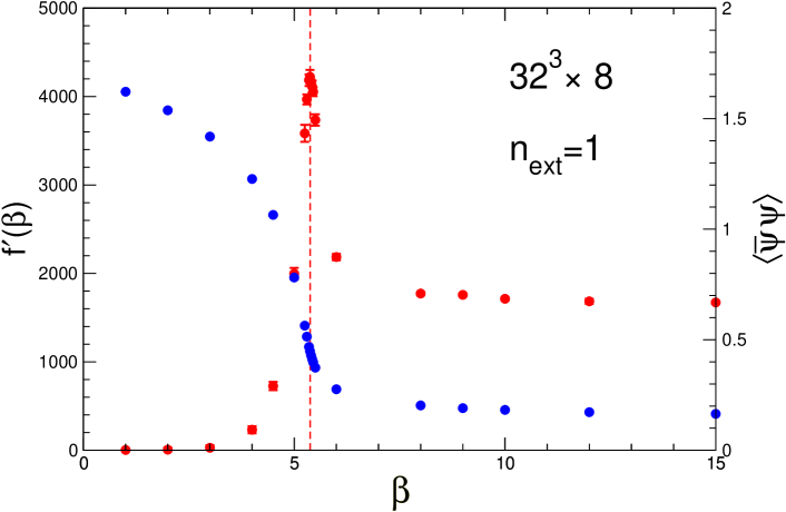
Figure 1: The derivative of the free energy eq. (7) with respect to the gauge coupling (left axis, blue circles), and the chiral condensate eq. (13) (right axis, red squares) versus $\beta$. The vertical line represents the position of the peak in the derivative of the free energy.

we show an example of $F^{\prime}$ measured for $n_{\text{ext}}=1$ on a $32^{3}\times 8$ lattice. In the same figure we display also the chiral condensate

$$\langle\bar{\psi}\psi\rangle=\langle\frac{1}{V}\,\frac{N_{f}}{4}\,\,\text{Tr}\,M^{-1}\rangle$$ (13)

and the numerical data point out that the peak in the derivative of the free energy corresponds to the drop in the chiral condensate, the latter is a signal of the transition leading to chiral symmetry restoration.

In figure 2

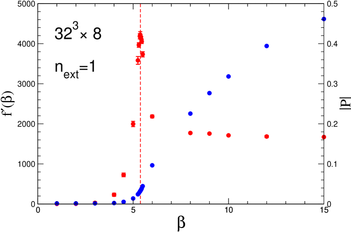
Figure 2: The derivative of the free energy as in figure 1 together with the absolute value of the Polyakov loop eq. (14). Vertical dotted line as in figure 1.

we compare the derivative of the free energy with the absolute value of the Polyalov loop

$$P=\frac{1}{V_{s}}\sum_{\vec{x}}\frac{1}{3}\,{\text{Tr}}\prod_{x_{4}=1}^{L_{t}}U_{4}(x_{4},\vec{x})\;.$$ (14)

We can see that also in this case the rise of the Polyakov loop (expected at the deconfining phase transition) corresponds to the peak of the derivative of the free energy. Moreover, in figure 3

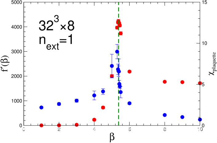
Figure 3: The derivative of the free energy as in figure 1 together with the susceptibility of the gauge action.

the derivative of the free energy is displayed together with the plaquette susceptibility (susceptibility of the gauge action). It is evident from this figure that, within our statistical uncertainties, the peaks of the two quantities coincide. Similar results are obtained by looking at the susceptibilities of the Polyakov loop and of the chiral condensate.

From the above arguments we may draw some partial conclusions: the critical coupling of the phase transition can be located by looking at the peak of the derivative of the free energy; moreover, as in the case of zero external field and within statistical uncertainties, a single transition seems to be present where both deconfinement and chiral symmetry restoration take place.

It is worth to note that since the measurement of the derivative of the free energy is simply related to the measurement of the gauge plaquette we may have a good evaluation of the critical coupling with a relatively small sample of measurements.

As told before our aim is to find if the critical coupling depends on the strength of the applied constant chromomagnetic field. To this purpose we have varied the strength of the external field by tuning up the parameter $n_{\text{ext}}$ and we have searched for the phase transition signalled by the peak of the derivative of the free energy. We have found that indeed the critical coupling shifts towards lower values by increasing the external field strength. In figure 4

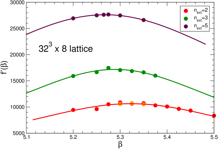
Figure 4: The derivative of the free energy eq. (7) versus $\beta$ for some values of the strength of the constant chromomagnetic field parameterized (see eq. (11)) by the integer $n_{\text{ext}}$. The yellow full circles corresponds to runs performed with different machines (APEmille) and algorithms as a check.

we display the derivative of the free energy in correspondence of three values of $n_{\text{ext}}$ obtained on a $32^{3}\times 8$ lattice, together with the fit curves given by eq. (12). As one can see the position of the peaks decreases by increasing the external field strength. In Table 1

Table 1: The values of the critical coupling versus the external field strengths.

lattice size	$n_{\text{ext}}$	$\beta_{c}$
$\qquad 32\times 32\times 32\times 8\qquad$	$\qquad 0\qquad$	5.4851 (202)
$\qquad 64\times 32\times 32\times 8\qquad$	$\qquad 1\qquad$	5.4288 (128)
$\qquad 32\times 32\times 32\times 8\qquad$	$\qquad 1\qquad$	5.3808 (128)
$\qquad 32\times 32\times 32\times 8\qquad$	$\qquad 2\qquad$	5.3228 (90)
$\qquad 32\times 32\times 32\times 8\qquad$	$\qquad 3\qquad$	5.2888 (44)
$\qquad 32\times 32\times 32\times 8\qquad$	$\qquad 4\qquad$	5.2659 (48)
$\qquad 32\times 32\times 32\times 8\qquad$	$\qquad 5\qquad$	5.2680 (38)

we report the values of the critical couplings versus $n_{\text{ext}}$.

Figure 5

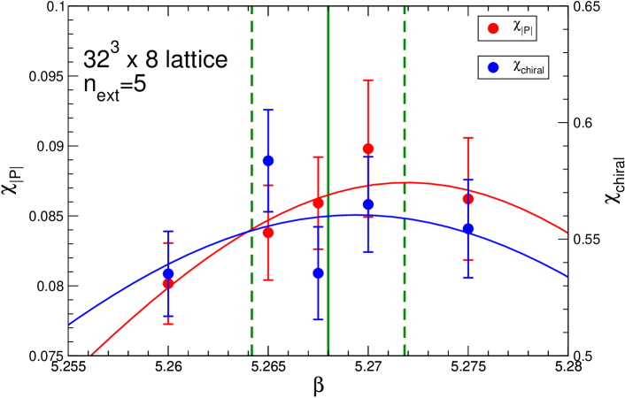
Figure 5: The susceptibility of the absolute value of the Polyakov loop together with the susceptibility of the chiral condensate. The vertical full line represents the position of the peak in the derivative of the free energy for chromomagnetic field strength $n_{\text{ext}}=5$. The vertical dotted lines give the error region. Red and blue full lines are the best fits with the same parameterization as in eq. (12) respectively to the susceptibility of the (absolute value of the) Polyakov loop and to that of the chiral condensate.

displays instead the susceptibility of the absolute value of the Polyakov loop together with the susceptibility of the chiral condensate in the peak region for the largest explored value of the external magnetic field ($n_{\text{ext}}=5$). It is worthwhile to note that, as mentioned earlier, the position of the peak of Polyakov loop susceptibility ($\beta=5.2719(164)$) and the position of the peak of the chiral condensate susceptibility ($\beta=5.2694(84)$) are consistent with each other and with the position of the peak obtained from the derivative of the free energy ($\beta=5.2680(38)$), thus confirming the conclusion stated above, i.e. that the chiral and the deconfinement transition are shifted towards lower temperatures by the presence of the external field in an equal way, i.e. they continue to be coincident within statistical errors even for $n_{\text{ext}}\neq 0$.

The numerical results obtained so far let us conclude that the critical coupling is dependent on the strength of the background constant chromomagnetic field. On the other hand for pure SU(3) gauge theory we obtained [22] that the value of the critical coupling is not changed by a monopole background field. Similar results are expected in presence of dynamical fermions [23, 16, 24], however we will verify this fact explicitly for the present case.

We recall the definition of an abelian monopole background field on the lattice, for more details and physical results see ref. [16]. It is well known that for SU(3) gauge theory the maximal abelian group is U(1)$\times$U(1), therefore we may introduce two independent types of abelian monopoles using respectively the Gell-Mann matrices $\lambda_{3}$ and $\lambda_{8}$ or their linear combinations. In the following we shall consider the abelian monopole field related to the $\lambda_{3}$ diagonal generator. In the continuum the abelian monopole field is given by

$$g\vec{b}^{a}({\vec{x}})=\delta^{a,3}\frac{n_{\mathrm{mon}}}{2}\frac{\vec{x}\times\vec{n}}{|\vec{x}|(|\vec{x}|-\vec{x}\cdot\vec{n})}\,,$$ (15)

where $\vec{n}$ is the direction of the Dirac string and, according to the Dirac quantization condition, $n_{\text{mon}}$ is an integer. The lattice links corresponding to the abelian monopole field eq. (15) are (we choose $\vec{n}=\hat{x}_{3}$)

$$\begin{split}U_{1,2}^{\text{ext}}(\vec{x})&=\begin{bmatrix}e^{i\theta^{\text{mon}}_{1,2}(\vec{x})}&0&0\\ 0&e^{-i\theta^{\text{mon}}_{1,2}(\vec{x})}&0\\ 0&0&1\end{bmatrix}\,\\ U^{\text{ext}}_{3}(\vec{x})&={\mathbf{1}}\,,\end{split}$$ (16)

with $\theta^{\text{mon}}_{1,2}(\vec{x})$ defined as

$$\begin{split}\theta^{\text{mon}}_{1}(\vec{x})&=-\frac{an_{\text{mon}}}{4}\frac{(x_{2}-X_{2})}{|\vec{x}_{\text{mon}}|}\frac{1}{|\vec{x}_{\text{mon}}|-(x_{3}-X_{3})}\,,\\ \theta^{\text{mon}}_{2}(\vec{x})&=+\frac{an_{\text{mon}}}{4}\frac{(x_{1}-X_{1})}{|\vec{x}_{\text{mon}}|}\frac{1}{|\vec{x}_{\text{mon}}|-(x_{3}-X_{3})}\,,\end{split}$$ (17)

where $(X_{1},X_{2},X_{3})$ are the monopole coordinates, $\vec{x}_{\text{mon}}=(\vec{x}-\vec{X})$. The monopole background field is introduced by constraining (see eq. (16)) the spatial links exiting from the sites at the boundary of the time slice $x_{t}=0$. For what concern spatial links exiting from sites at the boundary of other time slices ($x_{t}\neq 0$) we constrain these links according to eq. (16).

We have performed numerical simulations in presence of an abelian monopole background field with monopole charge $n_{\text{mon}}=10$ (again for 2 staggered flavors QCD of mass $am_{q}=0.075$). The critical coupling has been located by looking at the

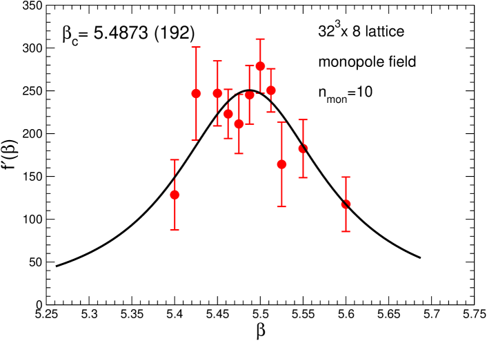
Figure 6: The derivative of the free energy for the abelian monopole background field eq. (15 in the peak region, together with (full line) the best fit eq. (12).

peak of the derivative of the free energy (see figure (6)). We find

$$\beta_{c}=5.4873(192)\,.$$ (18)

We have also done simulations in absence of any external chromomagnetic field, finding that the susceptibilities of the Polyakov loop, of the chiral condensate and of the plaquette display a peak at

$$\beta_{c}=5.495(25)\;.$$ (19)

Noticeably, this value of the critical coupling without external field is consistent, within our statistical uncertainty, with the value we get when we consider an abelian monopole field as background field. Therefore we can conclude that, as we found [16] in the case of pure gauge SU(3) gauge theory, the abelian monopole field has no effect on the position of the critical coupling.

4 Deconfinement temperature and critical field strength

In previous studies [2] in pure lattice gauge theories we looked for the possible dependence of the deconfinement temperature on the strength of an external (chromo)magnetic field. In particular we studied SU(2), and SU(3) l.g.t.’s both in (2+1) and (3+1) dimensions and U(1) l.g.t. both in 4 dimensions and in (2+1) dimensions. In fact, in the case of non-abelian gauge theories, irrespective of the number of dimensions, we found that the deconfinement temperature depends on the strength of the constant chromomagnetic background field (similar studies have been performed within a different framework in refs. [25, 26]). On the other hand, for U(1) gauge theory we found no evidence for a dependence of the critical coupling on the strength of an external magnetic field. In particular, as is well known, 4-dimensional U(1) l.g.t. undergoes a transition from a confined phase to a Coulomb phase: our analysis showed [2] that the location of the confinement-Coulomb phase transition is not changed by varying the strength of an applied constant magnetic field. The same analysis has been performed for compact quantum electrodynamics in (2+1) dimensions where it is known [27] that at zero temperature external charges are confined for all values of the coupling and it is well ascertained that the confining mechanism is the condensation of magnetic monopoles which gives rise to a linear confining potential and a non-zero string tension. Even in this case we verified that the critical temperature for deconfinement does not depend on the strength of an external magnetic field. As a consequence, we concluded that the dependence of the critical coupling on the strength of the external chromomagnetic field is a peculiar feature of non-abelian theories.

The main aim of the present investigation is to extend our study to non-abelian gauge theories in presence of dynamical fermions. To this end, having determined in the previous section the critical couplings corresponding to different external field strengths, we now try to estimate the critical temperature:

$$T_{c}=\frac{1}{a(\beta_{c},m_{q})L_{t}}\,,$$ (20)

where $L_{t}$ is the lattice temporal size and $a(\beta_{c},m_{q})$ is the lattice spacing at the given critical coupling $\beta_{c}$. In the case of SU(3) pure gauge theory in order to evaluate $a(\beta_{c})$ we used [2] the string tension. We obtained that the values of the critical temperature versus the square root of the external field strength can be fitted by a linear parameterization. By extrapolating to zero external field strength we obtained:

$$\frac{T_{c}(0)}{\sqrt{\sigma}}=0.643(15)$$ (21)

in very good agreement with the estimate $T_{c}/\sqrt{\sigma}=0.640(15)$ in the literature [28]. At the same time the intercept of line with the zero temperature axis furnished an estimate of the critical field strength (i.e. the limit value above which the gauge system is in the deconfined phase even at very low temperatures)

$$\sqrt{gH_{c}}=(2.63\pm 0.15)\sqrt{\sigma}=(1.104\pm 0.063){\text{ GeV}}=6.26(2)\times 10^{19}\text{ Gauss}$$ (22)

using for the physical value of the string tension $\sqrt{\sigma}=420\text{ MeV}$. The same analysis can be performed by means of the improved lattice scale introduced in Refs. [29, 30]

$$\widetilde{\Lambda}=\frac{1}{a}f(g^{2})(1+c_{2}\hat{a}(g)^{2}+c_{4}\hat{a}(g)^{4})\,,\;\;\hat{a}(g)\equiv\frac{f(g^{2})}{f(g^{2}=1)}$$ (23)

where $g$ is the gauge coupling, $c_{2}=0.195(16)$, $c_{4}=0.0562(45)$, $\widetilde{\Lambda}/\sqrt{\sigma}=0.0138(12)$ and $f(g^{2})$ is the 2-loop scaling function

$$f(g^{2})=(b_{0}g^{2})^{-b_{1}/2b_{0}^{2}}\,\,\exp\left(-\frac{1}{2b_{0}g^{2}}\right)$$ (24)

with

$$\begin{split}&b_{0}=\frac{1}{16\pi^{2}}\left[11\frac{N_{c}}{3}-\frac{2}{3}N_{f}\right]\\ &b_{1}=\left(\frac{1}{16\pi^{2}}\right)^{2}\left[\frac{34}{3}N_{c}^{2}-\left(\frac{10}{3}N_{c}+\frac{N_{c}^{2}-1}{N_{c}}\right)N_{f}\right]\,;\end{split}$$ (25)

$N_{c}$ is the number of colors and $N_{f}$ is the number of flavors.

Obviously the analysis of pure gauge data in units of $\widetilde{\Lambda}$ gives results consistent with the same analysis done using the scale of the string tension (see Ref. [2]). In particular a linear extrapolation towards zero external field gives:

$$\frac{T_{c}}{\widetilde{\Lambda}}=45.05(1.02)$$ (26)

in agreement with $T_{c}/\widetilde{\Lambda}=46.38(1.09)$ obtained from $T_{c}/\sqrt{\sigma}=0.640(15)$. Moreover the critical field strength turns out to be

$$\frac{\sqrt{gH_{c}}}{\widetilde{\Lambda}}=209.6\pm 3.07$$ (27)

which corresponds to $\sqrt{gH_{c}}=1.21(11)GeV$ in agreement with the estimate $\sqrt{gH_{c}}=1.10(6)GeV$ given in eq. (22).

Let us turn now to the $N_{f}=2$ case. Also in this case we have to face the problem of fixing the physical scale. In order to reduce the systematic effects involved in this procedure we will consider the ratios

$$\frac{T_{c}(gH)}{T_{c}}\qquad\text{vs.}\qquad\frac{\sqrt{gH}}{T_{c}}$$ (28)

where $T_{c}$ is the critical temperature without external field. The above quantities can be obtained once the ratio of the lattice spacings at the respective couplings is known. A rough estimate of this ratio can be inferred by using the 2-loop scaling function $f(g^{2})$ given in eq. (24) for $N_{f}=2$. A better estimate could be obtained, as in the quenched case, by adopting an improved scaling function $f(g^{2})(1+c_{2}\hat{a}(g)^{2}+c_{4}\hat{a}(g)^{4})$. We do not know, however, the values of $c_{2}$ and $c_{4}$ for $N_{f}=2$. In a first approximation we will fix $c_{2}$ and $c_{4}$ to their quenched values given above. In figure 7

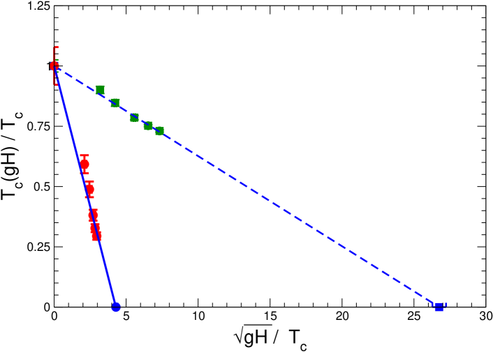
Figure 7: The critical temperature $T_{c}(gH)$ at a given strength of the chromomagnetic background field in units of the critical temperature $T_{c}$ without external field versus the square root of the strength of the background field in the same units. Red circles are obtained by adopting the improved scaling function. The blue line is the linear best fit. The blue circle on the horizontal axis is the linear extrapolated values for the critical background field. Green squares are obtained by adopting the 2-loop scaling function. The blue dashed line is the linear best fit. The blue square on the horizontal axis is the linear extrapolated values for the critical field.

the quantities reported in eq. (28) are displayed for both choices described above, i.e. 2-loop asymptotic scaling and improved scaling.

The main result of our investigation is clear: even in presence of dynamical quarks the critical temperature decreases with the strength of the chromomagnetic field; moreover a linear fit to our data can be extrapolated to very low temperatures, leading to the prediction of a critical field strength above which strongly interacting matter should be deconfined at all temperatures.

However, as can be appreciated from figure 7, the exact value of the critical field strength is largely dependent on the choice of the physical scale. In particular, assuming the 2-loop scaling function we obtain

$$\frac{\sqrt{gH_{c}}}{T_{c}}=26.8(5)\,,$$ (29)

while assuming the improved scaling function we obtain

$$\frac{\sqrt{gH_{c}}}{T_{c}}=4.29(10)\,.$$ (30)

If the deconfinement temperature at zero field strength is taken to be of the order of $170$ MeV, that means $\sqrt{gH_{c}}$ in the range $0.7-4.5$ GeV.

It is clear that in order to get a reliable estimate of the critical field strength, suitable for phenomenological purposes, one should get a more reliable estimate of the physical scale of our lattices. However one should work at a fixed value of the pion mass (as close as possible to its physical value) as well: that is beyond the purpose of the present investigation and will be the subject of further studies.

To conclude this section we consider our measurements of the chiral condensate. In figure 8

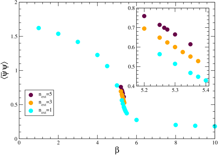
Figure 8: The chiral condensate eq. (13) versus $\beta$ in correspondence of some values of the constant chromomagnetic background field. In the inset the region corresponding to the phase transition has been magnified.

we display the chiral condensate versus the gauge coupling in correspondence of some values of the external field strength. Our numerical data show that, at least in the critical region, the value of the chiral condensate depends on the strength of the applied field. Interestingly enough, similar results for the chiral condensate have been found in ref. [31].

5 Summary and Conclusions

In this paper we have studied how a constant chromomagnetic field perturbs the QCD dynamics. In particular we focused on the theory at finite temperature and we have found that, analogously to what happens in the pure gauge theory [2], the critical temperature depends on the strength of the constant chromomagnetic background field: it decreases as the external field is increased and we have inferred, as an extrapolation of our results, that eventually the system is always deconfined for strong enough field strengths. We estimated this critical field strength to be of the order of 1 GeV, which is a typical QCD scale [32]. Notice that our estimate is of course affected by several systematic uncertainties, like that regarding the estimate of the physical scale: for that reason we consider it only as an order of magnitude of the real expected critical strength. In fact a more reliable determination usable for phenomenological purposes should be performed by working with a fixed physical value of the pion mass (and as close as possible to its physical value); that is out of the purpose of the present work and will be the subject of future investigations.

By comparing the critical couplings determined from the derivative of the free energy functional with those determined from the susceptibility of the chiral condensate and of the Polyakov loop we have ascertained that, even in presence of an external chromomagnetic background field and at least up to the field strengths explored in the present work, the critical temperatures where deconfinement and chiral symmetry restoration take place coincide within errors.

Another intriguing aspect we have found is the dependence of the chiral condensate on the chromomagnetic field strength. This last point deserves further studies. In order to get a deeper understanding of our results, we also plan to study the effect of the background field on the equation of state of QCD.

References

- [1] P. Cea and L. Cosmai, Abelian chromomagnetic fields and confinement, JHEP 02 (2003) 031, [hep-lat/0204023].
- [2] P. Cea and L. Cosmai, Color dynamics in external fields, JHEP 08 (2005) 079, [hep-lat/0505007].
- [3] F. Karsch and M. Lutgemeier, Deconfinement and chiral symmetry restoration in an SU(3) gauge theory with adjoint fermions, Nucl. Phys. B550 (1999) 449–464, [hep-lat/9812023].
- [4] J. Engels, S. Holtmann, and T. Schulze, The chiral transition of N(f) = 2 QCD with fundamental and adjoint fermions, PoS LAT2005 (2006) 148, [hep-lat/0509010].
- [5] G. Lacagnina, G. Cossu, M. D’Elia, A. Di Giacomo, and C. Pica, Monopole condensation in two-flavour adjoint QCD, hep-lat/0609049.
- [6] L. McLerran and R. D. Pisarski, Phases of Cold, Dense Quarks at Large , arXiv:0706.2191 [hep-ph].
- [7] S. Hands, S. Kim, and J.-I. Skullerud, Deconfinement in dense 2-color QCD, Eur. Phys. J. C48 (2006) 193, [hep-lat/0604004].
- [8] B. Alles, M. D’Elia, and M. P. Lombardo, Behaviour of the topological susceptibility in two colour QCD across the finite density transition, Nucl. Phys. B752 (2006) 124–139, [hep-lat/0602022].
- [9] S. Conradi, A. D’Alessandro, and M. D’Elia, Confining properties of QCD at finite temperature and density, arXiv:0705.3698 [hep-lat].
- [10] P. Cea, L. Cosmai, and A. D. Polosa, The lattice Schrödinger functional and the background field effective action, Phys. Lett. B392 (1997) 177–181, [hep-lat/9601010].
- [11] P. Cea and L. Cosmai, Probing the non-perturbative dynamics of SU(2) vacuum, Phys. Rev. D60 (1999) 094506, [hep-lat/9903005].
- [12] M. Lüscher, R. Narayanan, P. Weisz, and U. Wolff, The Schrödinger functional: A renormalizable probe for non Abelian gauge theories, Nucl. Phys. B384 (1992) 168–228, [hep-lat/9207009].
- [13] M. Lüscher and P. Weisz, Background field technique and renormalization in lattice gauge theory, Nucl. Phys. B452 (1995) 213–233, [hep-lat/9504006].
- [14] G. C. Rossi and M. Testa, The structure of Yang-Mills theories in the temporal gauge. 1. General formulation, Nucl. Phys. B163 (1980) 109.
- [15] D. J. Gross, R. D. Pisarski, and L. G. Yaffe, QCD and instantons at finite temperature, Rev. Mod. Phys. 53 (1981) 43.
- [16] P. Cea, L. Cosmai, and M. D’Elia, The deconfining phase transition in full QCD with two dynamical flavors, JHEP 02 (2004) 018, [hep-lat/0401020].
- [17] P. de Forcrand, M. D’Elia, and M. Pepe, A study of the ’t Hooft loop in SU(2) Yang-Mills theory, Phys. Rev. Lett. 86 (2001) 1438, [hep-lat/0007034].
- [18] M. D’Elia and L. Tagliacozzo, Direct numerical computation of disorder parameters, Phys. Rev. D74 (2006) 114510, [hep-lat/0609018].
- [19] L. Del Debbio, A. Di Giacomo, and G. Paffuti, Detecting dual superconductivity in the ground state of gauge theory, Phys. Lett. B349 (1995) 513–518, [hep-lat/9403013].
- [20] S. Gottlieb, W. Liu, D. Toussaint, R. L. Renken, and R. L. Sugar, Hybrid molecular dynamics algorithms for the numerical simulation of quantum chromodynamics, Phys. Rev. D35 (1987) 2531–2542.
- [21] E. Laermann and O. Philipsen, Status of lattice QCD at finite temperature, Ann. Rev. Nucl. Part. Sci. 53 (2003) 163–198, [hep-ph/0303042].
- [22] P. Cea, L. Cosmai, and M. D’Elia, Investigations on the deconfining phase transition in QCD, Nucl. Phys. Proc. Suppl. 129 (2004) 751–753, [hep-lat/0309031].
- [23] J. M. Carmona, M. D’Elia, L. Del Debbio, A. Di Giacomo, B. Lucini, and G. Paffuti, Color confinement and dual superconductivity in full QCD, Phys. Rev. D66 (2002) 011503, [hep-lat/0205025].
- [24] M. D’Elia, A. Di Giacomo, B. Lucini, G. Paffuti, and C. Pica, Color confinement and dual superconductivity of the vacuum. IV, Phys. Rev. D71 (2005) 114502, [hep-lat/0503035].
- [25] V. Skalozub and M. Bordag, Colour ferromagnetic vacuum state at finite temperature, Nucl. Phys. B576 (2000) 430–444, [hep-ph/9905302].
- [26] V. Demchik and V. Skalozub, The spontaneous generation of magnetic fields at high temperature in SU(2)-gluodynamics on a lattice, hep-lat/0601035.
- [27] A. M. Polyakov, Quark confinement and topology of gauge groups, Nucl. Phys. B120 (1977) 429–458.
- [28] M. J. Teper, Glueball masses and other physical properties of SU(N) gauge theories in D = 3+1: a review of lattice results for theorists, hep-th/9812187.
- [29] C. R. Allton, Lattice Monte Carlo data versus perturbation theory, hep-lat/9610016.
- [30] R. G. Edwards, U. M. Heller, and T. R. Klassen, Accurate scale determinations for the Wilson gauge action, Nucl. Phys. B517 (1998) 377–392, [hep-lat/9711003].
- [31] J. Alexandre, K. Farakos, S. J. Hands, G. Koutsoumbas, and S. E. Morrison, QED(3) with dynamical fermions in an external magnetic field, Phys. Rev. D64 (2001) 034502, [hep-lat/0101011].
- [32] D. Kabat, K.-M. Lee, and E. Weinberg, QCD vacuum structure in strong magnetic fields, Phys. Rev. D66 (2002) 014004, [hep-ph/0204120].