Balancing Local Order and Long-Ranged Interactions in the Molecular Theory of Liquid Water

Abstract

A molecular theory of liquid water is identified and studied on the basis of computer simulation of the TIP3P model of liquid water. This theory would be exact for models of liquid water in which the intermolecular interactions vanish outside a finite spatial range, and therefore provides a precise analysis tool for investigating the effects of longer-ranged intermolecular interactions. We show how local order can be introduced through quasi-chemical theory. Long-ranged interactions are characterized generally by a conditional distribution of binding energies, and this formulation is interpreted as a regularization of the primitive statistical thermodynamic problem. These binding-energy distributions for liquid water are observed to be unimodal. The gaussian approximation proposed is remarkably successful in predicting the Gibbs free energy and the molar entropy of liquid water, as judged by comparison with numerically exact results. The remaining discrepancies are subtle quantitative problems that do have significant consequences for the thermodynamic properties that distinguish water from many other liquids. The basic subtlety of liquid water is found then in the competition of several effects which must be quantitatively balanced for realistic results.

Introduction

On the basis of the temperature dependence of its macroscopic properties, liquid water belongs to a class of liquids often referred to as “associated liquids.” Fig. 1 gives one example of a characteristic distinction between liquid water and common organic solvents: the temperature dependence of the internal pressure. For van der Waals liquids, this temperature dependence is related directly to the temperature dependence of the liquid density. Organic solvents conform to this expectation, but liquid water exhibits a contrasting behavior, and that alternative behavior is attributed typically to the temperature dependence of water association through hydrogen bonding interactions.

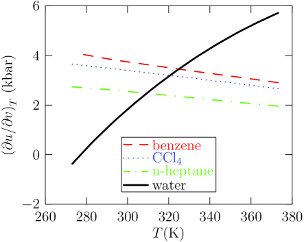
Figure 1: The internal pressure of several solvents as a function of temperature along their vapor saturation curve.Rowlinson and Swinton (1982) For van der Waals liquids $\left(\partial u/\partial v\right)_{T}\approx a\rho^{2}$. Organic solvents conform to this expectation, but water is qualitatively different.

As an associated liquid, water is regarded broadly also as a network liquid, though a definition of “network liquid” is usually not attempted. One aspect of the network view of liquid water is that models with defined short-ranged hydrogen bonding interactions that vanish precisely outside a finite range are designed specifically to study the network characteristics of that fluid. The work of Peery & EvansPeery and Evans (2003) gives a recent example that reviews and advances the forefront of statistical mechanical theory built explicitly on that network concept; this line of inquiry does indeed have an extended history, and the citations Andersen (1973, 1974); Dahl and Andersen (1983); Aranovich et al. (1999); Economou and Donohue (1991) give further examples. The finite range of interactions is a common feature of lattice-gas models of liquid water.Fleming and Gibbs (1974a, b); Stillinger (1975)

The theory investigated here is motivated by a simple, surprising result which can be regarded as a theorem for models with intermolecular interactions that vanish outside a radius $\lambda$, whether or not the liquid under consideration would be regarded as a network liquid on some other basis. Specifically, it is that the excess chemical potential is precisely

$$\beta\mu^{\mathrm{{ex}}}=\beta\mu^{\mathrm{{ex}}}_{\mathrm{{HS}}}\left(\lambda\right)+\ln p\left(n_{\lambda}=0\right)~{}.$$ (1)

This excess chemical potential $\mu^{\mathrm{{ex}}}$ is the Gibbs free energy per mole, in excess of the ideal contribution at the same density and temperature, of the one-component fluid considered. The thermodynamic temperature is $T=1/k\beta$ where $k$ is the Boltzmann’s constant, $\mu^{\mathrm{{ex}}}_{\mathrm{{HS}}}$ is the excess chemical potential for a hard-sphere solute, with $\lambda$ the distance of closest approach, at infinite dilution in the fluid. In the final term, $p\left(n_{\lambda}=0\right)$ is the probability that a specific actual molecule in the fluid has zero (0) neighbors within the radius $\lambda$.

After articulation, the theorem Eq. 1 is straightforwardly understood, and a simple proof is given below. As an orienting comment, we note that Eq. 1 has been useful already in the theory of the hard-sphere fluid.Beck et al. (2006) Of course, hard-sphere interactions are not involved literally in the interactions of physical systems, and it will transpire below that the hard-sphere contribution in Eq. 1 simply serves to organize the statistical information, not as an assumed feature of an underlying intermolecular potential model.

We emphasize that Eq. 1 is correct if intermolecular interactions vanish beyond the radius $\lambda$, independently of whether the liquid under consideration is a network liquid. Real network liquids have strong, short-ranged binding interactions, but invariably longer-ranged interactions as well. This paper investigates the simplest approximate extension of the Eq. 1 to real liquids, an extension which is realizable, and which is conceived on the basis of observable data, not from consideration of an assumed interaction model. The specific issues we address quantitatively include whether the effects of longer-than-near-neighbor interactions are simple for realistic models of liquid water, and whether reasonable values of $\lambda$ can be found that make the statistical theory of liquid water particularly simple with realistic intermolecular interactions.

Statistical Thermodynamic Theory

We seek $\mu^{\mathrm{{ex}}}$ on the basis of accessible simulation data. Since Eq. 1 contains $\mu^{\mathrm{{ex}}}_{\mathrm{{HS}}}$, we consider evaluating that quantity on the basis of simulation of the realistically modeled liquid of interest. For that purpose, the potential distribution theorem (PDT) Asthagiri et al. (in press 2007); Beck et al. (2006) difference formula yields

$$e^{-\beta(\mu^{\mathrm{{ex}}}_{\mathrm{{HS}}}-\mu^{\mathrm{{ex}}})}=p\left(n_{\lambda}=0\right)\int\limits_{-\infty}^{+\infty}P\left(\varepsilon|n_{\lambda}=0\right)e^{\beta\varepsilon}\mathrm{d}\varepsilon~{}.$$ (2)

If we take $\mu^{\mathrm{{ex}}}_{\mathrm{{HS}}}$ as known, Ashbaugh and Pratt (2006) Eq. (2) is an equation for $\mu^{\mathrm{{ex}}}$. $P\left(\varepsilon|n_{\lambda}=0\right)$ is the conditional probability of the binding energy of a specific molecule for the event that $n_{\lambda}=0$, i.e., the specific molecule considered has zero (0) neighbors within radius $\lambda$. $p\left(n_{\lambda}=0\right)$ is the marginal probability of that event. If the intermolecular interactions vanish for ranges as large as $\lambda$, those binding energies are always zero (0). This yields Eq. 1 under the assumptions noted.

For general interactions, we regard the conditioning of Eq. 2 when $\lambda>0$ as a regularization of the statistical problem embodied in Eq. (2) when $\lambda=0$, which is impossible on the basis of a direct calculation. After regularization, the statistical problem becomes merely difficult. For $\lambda\rightarrow\infty$, a gaussian distribution model for $P\left(\varepsilon|n_{\lambda}=0\right)$ should be accurate since then many solution elements will make small, weakly-correlated contributions to $\varepsilon$. The marginal probability $p\left(n_{\lambda}=0\right)$ becomes increasingly difficult to evaluate as $\lambda$ becomes large, however. For $\lambda$ on the order of molecular length scales typical of dense liquids, a simple gaussian model would accept some approximation error as the price for manageable statistical error. If $P\left(\varepsilon|n_{\lambda}=0\right)$ is modeled by a gaussian of mean $\left<\varepsilon|n_{\lambda}=0\right>$ and variance $\left<\delta\varepsilon^{2}|n_{\lambda}=0\right>$, then

$$\mu^{\mathrm{{ex}}}-\mu^{\mathrm{{ex}}}_{\mathrm{{HS}}}\left(\lambda\right)-kT\ln p\left(n_{\lambda}=0\right)-\left<\varepsilon|n_{\lambda}=0\right>\\ =\frac{1}{2kT}\left<\delta\varepsilon^{2}|n_{\lambda}=0\right>~{}.$$ (3)

We regard the formulation Eq. 3 merely as a parsimonious use of statistical information that might be obtained from a simulation record. This simple model motivates the following analyses.

An essentially thermodynamic derivation of Eq. 2, one that illustrates the connection with quasi-chemical theory, was given previously.Pratt and Asthagiri (2007) Our result there was formulated as

$$\beta\mu_{\alpha}^{\mathrm{ex}}=\beta\mu_{\alpha\mathrm{w}_{m=0}}^{\mathrm{ex}}-\ln\left(1+\sum_{m\geq 1}K_{m}\rho_{\mathrm{w}}{}^{m}\right)$$ (4)

where $\alpha$ indicates the distinguished molecule and ‘w’ the molecules of the solvent medium, for example water. Comparison of Eqs. 2 and 4 then suggests the identification

$$p\left(n_{\lambda}=0\right)=\frac{1}{1+\sum_{m\geq 1}K_{m}\rho_{\mathrm{w}}{}^{m}}~{}.$$ (5)

Thus the marginal probability of the event ($n_{\lambda}$ = 0) directly interrogates chemical contributions involving the chemical equilibrium ratios $K_{n}$’s on the basis of the assumed forcefield. This correspondence is indeed a basic result of constructive derivations of quasi-chemical theory.Paulaitis and Pratt (2002) Given adequate simulation data, explicit evaluation of individual $K_{n}$’s is not required. But more basic chemical analysis of the $K_{n}$’s, e.g., using electronic structure method,Martin et al. (1998); Pratt and Rempe (1999); Rempe and Pratt (2001); Rempe et al. (2000); Asthagiri et al. (2004); Asthagiri et al. (2003a); Asthagiri and Pratt (2003); Asthagiri et al. (2003b); Rempe et al. (2004) is not implemented either. We add for completeness that previous discussions denoted $p\left(n_{\lambda}=0\right)=x_{0}$, with $x_{n}\propto K_{n}\rho_{\mathrm{w}}{}^{n}$ the probability that the distinguished molecule has a coordination number of $n$, and $K_{0}\equiv$1.Pratt and Laviolette (1998); Pratt and Rempe (1999); Paulaitis and Pratt (2002); Beck et al. (2006); Pratt and Asthagiri (2007)

These equations correctly suggest that this formulation is fully general for the classical statistical thermodynamic problem considered. This formulation doesn’t make a lattice structural idealization, doesn’t assume that the interaction potential energy is pairwise decomposable, doesn’t assume that the interaction potential energy model provides a handy definition of ‘H-bonded,’ and the coordination definition — the occupancy within a radius $\lambda$ — is observational on the basis of molecular structure. Effective values of $\lambda$ should be established eventually on the basis of the statistical information secured.

Of course, the chemical potential provides the partial molar entropy

$$\left(\frac{\partial S}{\partial n_{\alpha}}\right)_{T,p}=\frac{1}{T}\left(\frac{\partial\left\langle E\right\rangle}{\partial n_{\alpha}}\right)_{T,p}+\frac{p}{T}\left(\frac{\partial\left\langle V\right\rangle}{\partial n_{\alpha}}\right)_{T,p}-\frac{\mu_{\alpha}}{T},$$ (6)

or for the one-component system considered here

$$\frac{S^{\mathrm{ex}}}{nk}=\frac{\left\langle\varepsilon\right\rangle}{2kT}+\left(\frac{p}{\rho kT}-1\right)-\frac{\mu^{\mathrm{ex}}}{kT}~{}.$$ (7)

On the right side the quantities $\left\langle\varepsilon\right\rangle$, and $p$ (the fluid pressure) are mechanical properties which are directly available from a simulation record.

It is an important but a tangential point that the distributions $P\left(\varepsilon|n_{\lambda}=0\right)$ to which this theory directs our attention are different from the $p(v)$ that have been frequently considered following the work of Rahman & Stillinger;Rahman and Stillinger (1971) see also the review of Stillinger.Stillinger (1980) $p(v)$ is the distribution with the interpretation that $\int_{v_{1}}^{v_{2}}p(v)\mathrm{d}v=n(v_{2},v_{1})$ is the number of molecules neighboring a particular one with pair interaction $v$ in the range $(v_{2},v_{1})$. $p(v)$ has been used to convey reasonable definitions of ‘H-bonded’ on the basis of simulation models of water, and it is well-designed for the purpose. It doesn’t supply the correlations that the distributions $P\left(\varepsilon|n_{\lambda}=0\right)$ use to determine the free energy.

Simulation Data

To test these ideas, 50000 snapshots from simulationsPaliwal et al. (2006); Paliwal (2005) performed at 298, 350 and 400 K were analyzed. Calculations of $\mu^{\mathrm{{ex}}}_{\mathrm{{HS}}}$ and $p(n_{\lambda}=0)$ were carried out as described by Paliwal, et al.Paliwal et al. (2006) The interaction energy of a water molecule was calculated as the sum of pairwise additive van der Waals and electrostatic energies. Lennard-Jones interactions were considered within 13 Å, and standard long range corrections were applied beyond this distance. Electrostatic interactions were evaluated using the Ewald summation method.

Statistical uncertainties in $\mu^{\mathrm{ex}}$ were computed by dividing the total number of snapshots into five blocks and evaluating block averages. For comparison, $\mu^{\mathrm{ex}}$ was determined from the histogram overlap method after evaluating also the uncoupled binding-energy distribution $P^{(0)}\left(\varepsilon\right)$,Beck et al. (2006) which was obtained by placing 5000 randomly oriented water molecules at randomly chosen locations in each snapshot. Table 1 collects the individual terms for the gaussian model, Eq. (3), at each temperature, and additionally the entropy evaluated from Eq. 7. The observed dependence on $\lambda$ of the free energy at each temperature is shown in Fig 3.

Table 1: Free energy contributions in kcal/mol associated with the gaussian model. The bottom value of each temperature set gives the corresponding free energy evaluated by the histogram overlap method. The rightmost column is the excess entropy per particle. Note that the entropy here raises the net free energy (see Eq. 7), and the magnitude of the entropy contribution $TS^{\mathrm{ex}}/n$ ranges here from 60-75% of the magnitude of the free energy $\mu^{\mathrm{ex}}$.

T(K)	$\lambda$ (nm)	$\mu^{\mathrm{ex}}_{\mathrm{HS}}\left(\lambda\right)$	$+kT\ln p\left(n_{\lambda}=0\right)$	$+\left\langle\varepsilon|n_{\lambda}=0\right\rangle$	$+\left\langle\delta\varepsilon^{2}|n_{\lambda}=0\right\rangle/2kT$	$=\mu^{\mathrm{ex}}$	$S^{\mathrm{ex}}/nk$
298	0.2600	2.93	-0.04	-19.74	9.87	-6.98 $\pm$ 0.02	-5.88
	0.2650	3.15	-0.13	-19.68	9.93	-6.73 $\pm$ 0.03	-6.30
	0.2675	3.25	-0.20	-19.59	9.97	-6.57 $\pm$ 0.04	-6.57
	0.2700	3.35	-0.31	-19.46	9.98	-6.44 $\pm$ 0.03	-6.79
	0.2725	3.45	-0.44	-19.27	9.97	-6.29 $\pm$ 0.03	-7.05
	0.2750	3.56	-0.60	-19.03	9.92	-6.15 $\pm$ 0.03	-7.28
	0.2775	3.67	-0.78	-18.73	9.83	-6.01 $\pm$ 0.04	-7.52
	0.2800	3.78	-0.98	-18.39	9.71	-5.88 $\pm$ 0.03	-7.74
	0.2900	4.23	-1.96	-16.75	8.89	-5.59 $\pm$ 0.04	-8.23
	0.3000	4.71	-3.09	-14.93	7.77	-5.54 $\pm$ 0.06	-8.31
	0.3100	5.22	-4.27	-13.21	6.67	-5.59 $\pm$ 0.18	-8.23
	0.3200	5.76	-5.45	-11.65	5.54	-5.80 $\pm$ 0.37	-7.87
	0.3300	6.32	-6.64	-10.30	4.78	-5.84 $\pm$ 0.97	-7.81
						-6.49	-6.71
350	0.2600	3.06	-0.05	-18.43	9.44	-5.98 $\pm$ 0.02	-5.65
	0.2625	3.15	-0.09	-18.41	9.46	-5.89 $\pm$ 0.02	-5.78
	0.2700	3.45	-0.33	-18.14	9.47	-5.55 $\pm$ 0.02	-6.27
	0.2750	3.66	-0.62	-17.73	9.35	-5.34 $\pm$ 0.02	-6.57
	0.2800	3.87	-0.99	-17.15	9.10	-5.17 $\pm$ 0.01	-6.82
	0.2900	4.32	-1.92	-15.67	8.24	-5.03 $\pm$ 0.04	-7.02
	0.3000	4.80	-3.00	-14.05	7.20	-5.05 $\pm$ 0.06	-6.99
	0.3100	5.29	-4.13	-12.48	6.14	-5.18 $\pm$ 0.10	-6.80
	0.3200	5.81	-5.28	-11.01	5.24	-5.24 $\pm$ 0.22	-6.72
	0.3300	6.36	-6.41	-9.74	4.47	-5.32 $\pm$ 0.45	-6.60
						-5.83	-5.87
400	0.2600	3.03	-0.06	-17.19	8.97	-5.25 $\pm$ 0.02	-5.21
	0.2625	3.13	-0.10	-17.16	8.99	-5.14 $\pm$ 0.03	-5.35
	0.2700	3.41	-0.35	-16.89	8.95	-4.88 $\pm$ 0.02	-5.67
	0.2750	3.61	-0.63	-16.49	8.80	-4.71 $\pm$ 0.03	-5.89
	0.2800	3.81	-0.98	-15.96	8.52	-4.61 $\pm$ 0.03	-6.01
	0.2900	4.23	-1.87	-14.60	7.69	-4.55 $\pm$ 0.05	-6.09
	0.3000	4.68	-2.89	-13.10	6.72	-4.59 $\pm$ 0.05	-6.04
	0.3100	5.14	-3.97	-11.64	5.78	-4.69 $\pm$ 0.06	-5.91
	0.3200	5.62	-5.06	-10.31	4.95	-4.80 $\pm$ 0.14	-5.77
	0.3300	6.13	-6.12	-9.12	4.27	-4.84 $\pm$ 0.18	-5.72
						-5.31	-5.13

Results

Fig. 2 shows that the unconditioned distribution $P\left(\varepsilon\right)$ displays positive skew, but the conditioning diminishes that skew perceptibly, as expected. $P\left(\varepsilon|n_{\lambda}=0\right)$ is least skewed for the largest $\lambda$. All of these results are qualitatively unlike the binding-energy distributions obtained for a two dimensional model of liquid water Andaloro and Sperandeo-Mineo (1990) which has been studied further.Haymet et al. (1996); Silverstein et al. (1998) That previous result is multi-modal, behavior not seen here.

The distributions $P\left(\varepsilon|n_{\lambda}=0\right)$ shown in Fig. 2 are also qualitatively unlike the pair interaction distributions $p(v)$ Rahman and Stillinger (1971); Stillinger (1980) which are different, as was discussed above.

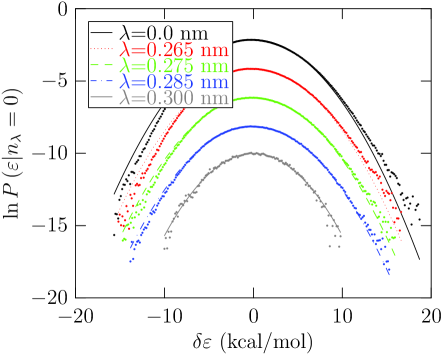
Figure 2: Probability density $P(\varepsilon|n_{\lambda}=0)$ of the binding energy of a water molecule in liquid water at 298 K. $\delta\varepsilon\equiv$ $\varepsilon-\left\langle\varepsilon|n_{\lambda}=0\right\rangle$, $\lambda$ = 0.0, …0.30 nm, from top to bottom with successive results shifted incrementally downward by 2 for clarity. The solid lines are the gaussian model for each data set.

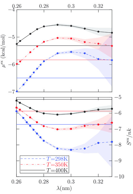
Figure 3: upper panel: Dependence of the free energy $\mu^{\mathrm{ex}}$ predicted by the gaussian model on the conditioning radius $\lambda$. The horizontal lines are the numerically exact results. The shaded areas indicate approximate 95% confidenc

The conditioning affects both the high-$\varepsilon$ and low-$\varepsilon$ tails of these distributions. The mean binding energy $\left\langle\varepsilon|n_{\lambda}=0\right\rangle$ increases with increasing $\lambda$ [Table 1], so we conclude that the conditioning eliminates low-$\varepsilon$ configurations more than high-$\varepsilon$ configurations that reflect less favorable interactions. Nevertheless, because of the exponential weighting of the integrand of Eq. (2) and the large variances, the high-$\varepsilon$ side of the distributions is overwhelmingly the more significant in this free energy prediction.

The fluctuation contribution exhibits a broad maximum for $\lambda<$ 0.29 nm, after which this contribution decreases steadily with increasing $\lambda$ [Table 1]. Evidently water molecules closest to the distinguished molecule, i.e., those closer than the principal maximum of oxygen-oxygen radial distribution function, don’t contribute importantly to the fluctuations. This is consistent with a quasi-chemical picture in which a water molecule and its nearest neighbors have a definite structural integrity. Fig. 4 shows $x_{n}\propto K_{n}\rho_{\mathrm{w}}{}^{n}$; the most probable coordination number is either 2 or 3 when $\lambda$=0.30 nm, but it is 4 when $\lambda$=0.33 nm. Nevertheless, the breadth of this distribution is remarkable. The coordination number $n$=6 is more probable than $n$=2 for the $\lambda$ = 0.33 nm results of Fig. 4.

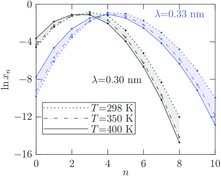
Figure 4: Coordination number probabilities, $x_{n}$ = $p\left(n_{\lambda}=n\right)$. Note that for $\lambda$=0.30 nm, the most probable coordination number is 2 or 3.Rahman and Stillinger (1971); Stillinger (1980) For $\lambda$=0.33 nm, the most probable coordination number is n=4. But $n$=4 and $n$=5 are nearly equally probable at $T$=298 K, and $n=6$ is then 17% of the whole. With the TIP3P model, as $T$ is lowered from 400 K to 298 K there is a clear tendency to enhance probability of higher coordination number cases.

The magnitude of the individual contributions to $\mu^{\mathrm{{ex}}}$ are of the same order as the net free energy; the mean binding energies are larger than that, as are the variance contributions in some cases. The variance contributions are about half as large as the mean binding energies, with opposite sign. It is remarkable and significant, therefore, that the net free energies at all temperatures are within roughly 12% of the numerically exact value computed by the histogram-overlap method. The predicted excess entropy, $S^{\mathrm{ex}}/nk$, (Fig. 3) is in error by 17% at the lowest temperature considered and more accurate than that at the higher temperatures. The constant-pressure heat capacity predicted by the model is roughly 30% larger than the result obtained using the numerically exact values for $S^{\mathrm{ex}}/nk$ in the same finite-difference estimate. A mean-field-like approximation that neglects fluctuations produces useless results.

The consistent combination of the various terms is an important observation. For example, the packing contribution, $\mu^{\mathrm{ex}}_{\mathrm{HS}}\left(\lambda\right)$, is sensitive to the interaction potential energy model used, and primarily through differences in the densities of different models at the higher temperatures.Paschek (2004) We found that use of values of $\mu^{\mathrm{ex}}_{\mathrm{HS}}\left(\lambda\right)$ corresponding to a more accurate model of liquid water Ashbaugh and Pratt (2006) spoils its consistency with the other contributions evaluated here with the TIP3P model, and that appreciably degrades the accuracy of the whole.

If $kT\ln{p(n_{\lambda}=0)}$ is zero [Table 1], the hard-sphere contribution $\mu^{\mathrm{{ex}}}_{\mathrm{{HS}}}\left(\lambda\right)$ is ill-defined. As a general matter, the sum $\mu^{\mathrm{{ex}}}_{\mathrm{{HS}}}\left(\lambda\right)+kT\ln{p(n_{\lambda}=0)}$ cannot be identified as a hard-sphere contribution. Since these terms have opposite signs, the net value can be zero or negative, and those possibilities are realized in Table 1. To define the hard-sphere contribution more generally, we require that $\mu^{\mathrm{{ex}}}_{\mathrm{{HS}}}\left(\lambda\right)$ be continuous as $p(n_{\lambda}=0)\rightarrow$ 1 with decreasing $\lambda$. All other terms of Eq.  (3) will be independent of $\lambda$ for values smaller than that, and it is natural to require that of $\mu^{\mathrm{{ex}}}_{\mathrm{{HS}}}\left(\lambda\right)$ also.

From Fig. 3, we see that $\lambda>$ 0.30 nm identifies a larger-size regime where the variation of the free energy with $\lambda$ is not statistically significant. Although we anticipate a decay toward the numerically exact value for $\lambda\rightarrow\infty$, the statistical errors become unmanageable for values of $\lambda$ much larger than 0.30 nm. When $\lambda$ = 0.30 nm a significant skew in $P(\varepsilon|n_{\lambda}=0)$ is not observed, as already noted with Fig. 2.

The predicted free energy $\mu^{\mathrm{{ex}}}$ is then distinctly above the numerically exact value, suggesting that the gaussian model predicts too much weight in the high-$\varepsilon$ tail. We further examined the high-$\varepsilon$ tail of $P\left(\varepsilon|n_{\lambda}=0\right)$ for larger values of $\lambda$ by carrying-out Monte Carlo calculations under the same conditions but with one water molecule carrying an O-centered sphere that prohibits other O-atoms within a radius $\lambda$. Those results are shown in Fig. 5. The accuracy of a gaussian model $P\left(\varepsilon|n_{\lambda}=0\right)$ is clearly born-out, but the gaussian model predicts slightly too much probability in the extreme high-$\varepsilon$ region particularly for $\lambda$ = 0.33 nm. The radial distribution of outer-shell neighbors in the conditioned sample (Fig. 6) shows that in that case the mean water-molecule-density is structured as a thin radial shell with roughly $n\approx$ 15 near-neighbors.

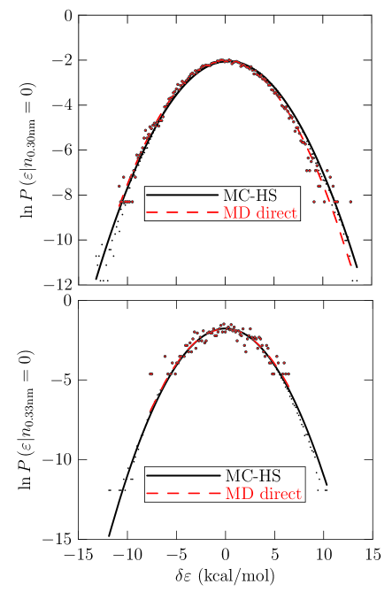
Figure 5: The fine black points are estimates of $P\left(\varepsilon|n_{\lambda}=0\right)$ obtained from Monte Carlo simulation of TIP3P water with one water molecule centering a hard-sphere which perfectly repels other water oxygens from a sphere of radius $\lambda$. (upper panel) $\lambda$ = 0.30 nm; (lower panel) $\lambda$ = 0.33 nm. The larger composite dots were obtained directly from molecular dynamics simulations with no constraint. The solid curve is the gaussian model for the expanded Monte Carlo data set, and confirms both the overall accuracy of the gaussian model and the estimated conditional mean and variance of Table I. Note that the data are slightly less than the gaussian model in the high-$\varepsilon$ tail. $T$=298K.

The design strategy here is that the theory should be correct in the $\lambda\rightarrow\infty$ limit. The accuracy of this approximate theory should then be judged for the largest values of $\lambda$ that are practical. Consulting the direct investigation of the high-$\varepsilon$ tail (Fig. 5), we see that the probability density drops off by roughly $\mathrm{e}^{-10}$ from the mode to the highest-$\varepsilon$ data there. But the integrand factor of $\mathrm{e}^{\beta\varepsilon}$ of Eq. 2 grows by roughly $\mathrm{e}^{+20}$ across that range; these distributions are remarkably wide even after the conditioning. Thus a statistical model that extends those data is still necessary.

In the context of implementations of quasi-chemical theory, it has been argued that the cut-off parameter $\lambda$ may be determined on a variational basis. Inner- and outer-shell contributions have countervailing effects, so where the net-results are insensitive to local changes of $\lambda$ distinct approximations may be considered well balanced.Beck et al. (2006) Here, the contributions corresponding to the inner-shell contribution in quasi-chemical theory are obtained numerically exactly so that argument isn’t compelling.

A previous quasi-chemical analysis of liquid water,Asthagiri et al. (2003c) which utilized ab initio molecular dynamics (AIMD) data, provides an interesting comparison with the present results. In initiating analysis of AIMD, that previous effort addressed a much more complicated case. Several contributions had to be estimated on the basis of slightly extraneous input, e.g., dielectric model calculations and rough estimates of the effects of outer-shell dispersion contributions. Nevertheless, there was some commonality in that both mean-field and fluctuation (dielectric) effects were involved in the outer-shell contributions. The net accuracy in that previous case was similar to that observed for the simpler case, more thoroughly analyzed here. The evaluated free energy was too high but by less than 1 kcal/mol at moderate temperatures.

Review of the theory Eq. 3 identifies a further remarkable observation. If we follow that logic in reverse, exploiting the fact that $\mu^{\mathrm{ex}}$ is an experimentally known quantity, then Eq. 3 provides a physically transparent theory for $\mu^{\mathrm{ex}}_{\mathrm{HS}}\left(\lambda\right)$ the object of central interest in theories of hydrophobic effects.Pratt (2002); Ashbaugh and Pratt (2006) As a theory of hydrophobic effects, Eq. 3 offers a specific accounting for the effects of the distinctive coordination characteristics of a water molecule in liquid water, and a specific accounting of the role of longer-than-near-neighbor-ranged interactions.

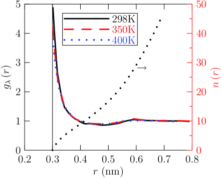
Figure 6: Distribution of water oxygen atoms radially from a distinguished water oxygen atom; evaluated with the sample corresponding to the condition $n_{\lambda}=0$, with $\lambda=$ 0.30 nm, for O-atom neighbors of the distinguished O-atom. The black, dotted curve is the running coordination number for the $T$=298K case.

Conclusions

Viewed from the perspective of Eq. 1, which is precisely correct for liquid water models with interactions shorter-ranged that $\lambda$, the quantitative contribution from longer-ranged interactions for the TIP3P model is essentially identical to the experimental value of $\mu^{\mathrm{{ex}}}$ for reasonable values of $\lambda\approx$ 0.33 nm, independently of temperature. If these longer-ranged contributions were modeled as a mean-field contribution $\left<\varepsilon|n_{\lambda}=0\right>$ only, the error would be nearly 100%. On the basis of the present work, it is evident that Ref. 35, in adopting the value $\lambda$ = 0.28 nm for $\mu^{\mathrm{{ex}}}_{\mathrm{{HS}}}\left(\lambda\right)$, assumed that quantitative chemical contributions reflecting short-ranged local order were negligible, independently of the local environment. This work then clarifies that for bulk water $\lambda$ = 0.26 nm, rather than 0.28 nm, if those chemical contributions are to be negligible. Moreover, suitable values of $\lambda$ require additional scrutiny for different local environments.

The present theory helps to gauge the significance of the various features of the interactions for the molecular of liquid water. As an example consider the case of an interaction model with near-neighbor-ranged interactions only. Then Eq. 1 applies. Suppose that the parameters of the model are adjusted to match precisely the observed coordination number probabilities (Fig. 4) for realistic models. If the packing contribution is obtained from physical dataHummer et al. (1996); Paschek (2004) or from simulation of realistic models of liquid water,Ashbaugh and Pratt (2006) then it will have positive magnitudes consistent with the values of Table 1. Then we must anticipate that the near-neighbor-ranged interaction model will yield errors in the free energy of roughly 100%. Contrapositively, if the parameters of such a model are adjusted to yield an accurate free energies, $\mu^{\mathrm{{ex}}}$ and $\mu^{\mathrm{{ex}}}_{\mathrm{{HS}}}\left(\lambda\right)$, the results above together with the theorem Eq. 1 suggest that the predicted coordination number distribution — specifically $p\left(n_{\lambda}=0\right)$ = $x_{0}$ — should differ significantly from results for models with realistic longer-ranged interactions. The implication of the analysis presented here for network models of liquid water is that a detailed treatment of local order alone – e.g., invoking specific short-ranged hydrogen-bonding interactions that capture geometric features of the tetrahedral structure of ice but not involving longer-ranged interactions – does not generally describe the range of thermodynamic properties that distinguishes water from organic solvents.

A more specific conclusion is that the observed $P\left(\varepsilon|n_{\lambda}=0\right)$ are unimodal. The gaussian model investigated here is surprisingly realistic; the molar excess entropies are predicted with an accuracy of magnitude roughly $k$ (Boltzmann’s constant). The predicted free energies are more accurate than 1 kcal/mol. The distinctions from gaussian form are subtle quantitative problems that have significant consequences for the thermodynamic properties that distinguish water from many other liquids. Those quantitative subtleties remain to be further analyzed.

References

- Peery and Evans (2003) T. B. Peery and G. T. Evans, J. Chem. Phys. 118, 2286 (2003).
- Andersen (1973) H. C. Andersen, J. Chem. Phys. 59, 4714 (1973).
- Andersen (1974) H. C. Andersen, J. Chem. Phys. 61, 4985 (1974).
- Dahl and Andersen (1983) L. W. Dahl and H. C. Andersen, J. Chem. Phys. 78, 1980 (1983).
- Aranovich et al. (1999) G. Aranovich, P. Donohue, and M. Donohue, J. Chem. Phys. 111, 2050 (1999).
- Economou and Donohue (1991) I. G. Economou and M. D. Donohue, AIChE J. 37, 1875 (1991).
- Fleming and Gibbs (1974a) P. D. Fleming and J. H. Gibbs, J. Stat. Phys. 10, 157 (1974a).
- Fleming and Gibbs (1974b) P. D. Fleming and J. H. Gibbs, J. Stat. Phys. 10, 351 (1974b).
- Stillinger (1975) F. H. Stillinger, in Adv. Chem. Phys. vol.31, “Non-simple liquids”, edited by S. Prigogine, I.; Rice (Chichester, Sussex, UK : Wiley, 1975), pp. 1 – 101.
- Beck et al. (2006) T. L. Beck, M. E. Paulaitis, and L. R. Pratt, The potential distribution theorem and models of molecular solutions (Cambridge University Press, Cambridge, 2006).
- Asthagiri et al. (in press 2007) D. Asthagiri, H. S. Ashbaugh, A. Piryatinski, M. E. Paulaitis, and L. R. Pratt, J. Am. Chem. Soc. 129, xyz (in press 2007).
- Ashbaugh and Pratt (2006) H. S. Ashbaugh and L. R. Pratt, Rev. Mod. Phys. 78, 159 (2006).
- Pratt and Asthagiri (2007) L. R. Pratt and D. Asthagiri, in Free Energy Calculations. Theory and Applications in Chemistry and Biology (Springer-Verlag, Berlin, 2007), chap. 9. Potential distribution methods and free energy models of molecular solutions, pp. 323–351.
- Paulaitis and Pratt (2002) M. E. Paulaitis and L. R. Pratt, Adv. Prot. Chem. 62, 283 (2002).
- Martin et al. (1998) R. L. Martin, P. J. Hay, and L. R. Pratt, J. Phys. Chem. A 102, 3565 (1998).
- Pratt and Rempe (1999) L. R. Pratt and S. B. Rempe, in Simulation and Theory of Electrostatic Interactions in Solution, edited by L. R. Pratt and G. Hummer (AIP Conference Proceedings, 1999), vol. 492, pp. 172–201.
- Rempe and Pratt (2001) S. B. Rempe and L. R. Pratt, Fluid Phase Equilibria 183-184, 121 (2001).
- Rempe et al. (2000) S. B. Rempe, L. R. Pratt, G. Hummer, J. D. Kress, R. L. Martin, and A. Redondo, J. Am. Chem. Soc. 122, 966 (2000).
- Asthagiri et al. (2004) D. Asthagiri, L. R. Pratt, M. E. Paulaitis, and S. B. Rempe, J. Am. Chem. Soc. 126, 1285 (2004).
- Asthagiri et al. (2003a) D. Asthagiri, L. R. Pratt, and H. S. Ashbaugh, J. Chem. Phys. 119, 2702 (2003a).
- Asthagiri and Pratt (2003) D. Asthagiri and L. R. Pratt, Chem. Phys. Letts. 371, 613 (2003).
- Asthagiri et al. (2003b) D. Asthagiri, L. R. Pratt, J. D. Kress, and M. A. Gomez, Chem. Phys. Letts. 380, 530 (2003b).
- Rempe et al. (2004) S. B. Rempe, D. Asthagiri, and L. R. Pratt, PCCP 6, 1966 (2004).
- Pratt and Laviolette (1998) L. R. Pratt and R. A. Laviolette, Mol. Phys. 94, 909 (1998).
- Rahman and Stillinger (1971) A. Rahman and F. H. Stillinger, J. Chem. Phys. 55, 3336 (1971).
- Stillinger (1980) F. H. Stillinger, Science 209, 451 (1980).
- Paliwal et al. (2006) A. Paliwal, D. Asthagiri, L. R. Pratt, H. S. Ashbaugh, and M. E. Paulaitis, J. Chem. Phys. 124 (2006).
- Paliwal (2005) A. Paliwal, Ph.D. thesis, Johns Hopkins University (2005).
- Andaloro and Sperandeo-Mineo (1990) G. Andaloro and R. M. Sperandeo-Mineo, Eur. J. Phys. 11, 275 (1990).
- Haymet et al. (1996) A. D. J. Haymet, K. A. T. Silverstein, and K. A. Dill, Faraday Discussions 103, 117 (1996).
- Silverstein et al. (1998) K. A. T. Silverstein, A. D. J. Haymet, and K. A. Dill, J. Am. Chem. Soc. 120, 3166 (1998).
- Paschek (2004) D. Paschek, J. Chem. Phys. 120, 6674 (2004).
- Asthagiri et al. (2003c) D. Asthagiri, L. R. Pratt, and J. D. Kress, Phys. Rev. E 68, 041505 (2003c).
- Pratt (2002) L. R. Pratt, Ann. Rev. Phys. Chem. 53, 409 (2002).
- Hummer et al. (1996) G. Hummer, S. Garde, A. E. García, A. Pohorille, and L. R. Pratt, Proc. Natl. Acad. Sci. USA 93, 8951 (1996).
- Rowlinson and Swinton (1982) J. S. Rowlinson and F. L. Swinton, Liquids and Liquid Mixtures (Butterworths, NY, 1982).