Hybridisation in Hubbard models with different bandwidths

Abstract

We investigate the orbital selective Mott transition in two-band Hubbard models by means of the Gutzwiller variational theory. In particular, we study the influence of a finite local hybridisation between electrons in different orbitals on the metal-insulator transition.

1 Introduction

Metal-insulator transitions in Hubbard models with different densities of states have attracted a lot of interest in recent years [1-10]. A dispute arose over the question whether or not the transition occurs at different interaction strengths for the wide and the narrow band. A transition with different critical interaction parameters is usually denoted as an ‘orbital selective Mott transition’ (OSMT). Apparently, a consensus has been reached that such an OSMT can occur in Hubbard models with different bandwidths, subject to the bandwidth ratio $\alpha$ of the narrow and the wide band and the value of the local exchange interaction $J$.

In most of the calculations in [1-10] the dynamical mean-field theory has been employed. We will use multiband Gutzwiller wave functions in order to study the OSMT. Such wave functions were originally introduced by Gutzwiller [11] in order to study ferromagnetism in the one-band Hubbard model. The evaluation of expectation values for the Gutzwiller wave function poses a difficult many-particle problem. Therefore, Gutzwiller, in his original work, used an approximation based on quasi-classical counting arguments [12, 13]. This ‘Gutzwiller approximation’ later turned out to be equivalent to an exact evaluation of expectation values in the limit of infinite spatial dimension or infinite coordination number. Generalised Gutzwiller wave function for multi-band Hubbard models have first been introduced and evaluated in the limit of infinite spacial dimensions in reference [15]. The formalism was further generalised, e.g., for superconducting systems, in references [16, 17].

The OSMT in a two-band Hubbard model has first been investigated by means of the Gutzwiller theory in reference [9]. In that work the authors found an OSMT both for vanishing ($J=0$) as well as for finite ($J\neq 0$) local exchange interaction. For $J=0$ the critical band width ratio was found to be $\alpha_{c}=0.2$. The Gutzwiller results in [9] were in good agreement with data from DMFT and a slave-spin approach proposed in reference [7].

In this work we will analyse the OSMT in a two-band model in more detail. In particular, we permit a finite expectation value $\Delta_{0}=\langle\hat{c}_{i,1}^{\dagger}\hat{c}_{i,2}\rangle$ for the local hybridisation which can change the nature of the OSMT. Such a hybridisation could be finite spontaneously, solely due to the Coulomb interaction, or due to a finite hybridisation term in the Hamiltonian. We will investigate both possibilities.

Our paper is organised as follows: The two-band Hubbard models are introduced in section 2. In section 3 we define generalised Gutzwiller wave functions and give the results for the variational ground-state energy for these wave functions in the limit of infinite spatial dimensions. The orbital selective Mott transition in a two-band model without a finite local hybridisation is discussed numerically, and as far as possible analytically, in section 4. In section 5 we investigate analytically the spontaneous hybridisation in a spinless two-band model. Finally, the hybridisation effects in the full two-band are studied in section 6, and a summary closes our presentation in section 7.

2 Model systems

In this work we investigate the two-band Hubbard model

$$\hat{H}=\sum_{i,j;b;\sigma}t^{b}_{i,j}\hat{c}^{\dagger}_{i,b,\sigma}\hat{c}_{j,b,\sigma}+\sum_{i}\hat{H}_{i;{\rm at}}=\hat{H}_{0}+\hat{H}_{\rm loc}\;.$$ (1)

Here, the one particle Hamiltonian $\hat{H}_{0}$ describes the hopping of electrons with spin $\sigma$ on a lattice with $L$ sites. The index $b=1,2$ labels the two degenerate orbitals at each lattice site. We assume that the hopping amplitudes

$$t^{b}_{i,j}=\alpha_{b}t_{i,j}$$ (2)

depend on the orbital index $b$ only via overall bandwidth factors $\alpha_{b}$. This leads to an orbital-dependent renormalisation

$$D_{b}(\varepsilon)=\frac{1}{\alpha_{b}}D_{0}\left(\frac{\varepsilon}{\alpha_{b}}\right)$$ (3)

of the bare density of states

$$D_{0}(\varepsilon)=\frac{1}{L}\sum_{k}\delta(\varepsilon-\varepsilon_{k})\;,$$ (4)

where $\varepsilon_{k}$ is the Fourier-transform of $t_{i,j}$. Throughout this work, only symmetric densities of states will be considered $D_{0}(-\varepsilon)=D_{0}(\varepsilon)$.

We will study the two-band model (1) with and without spin-degrees of freedom. For the full two-band model we assume that the orbitals have an $e_{\rm g}$-symmetry. The atomic Hamiltonian then reads

$$\hat{H}^{(2)}_{\rm{at}} = U\sum_{b}\hat{n}_{b,\uparrow}\hat{n}_{b,\downarrow}+U^{\prime}\sum_{\sigma,\sigma^{\prime}}\hat{n}_{1,\sigma}\hat{n}_{2,\sigma^{\prime}}-J\sum_{\sigma}\hat{n}_{1,\sigma}\hat{n}_{2,\sigma}$$

$$-J\sum_{\sigma}\hat{c}^{\dagger}_{1,\sigma}\hat{c}_{2,-\sigma}^{\phantom{+}}\hat{c}^{\dagger}_{1,-\sigma}\hat{c}_{2,\sigma}^{\phantom{+}}-J_{C}(\hat{c}^{\dagger}_{1,\uparrow}\hat{c}^{\dagger}_{1,\downarrow}\hat{c}_{2,\downarrow}^{\phantom{+}}\hat{c}_{2,\uparrow}^{\phantom{+}}+{\rm h.c.})$$

where in cubic symmetry the two parameters $U^{\prime}$ and $J_{C}$ are determined by $U^{\prime}=U-2J$ and $J_{C}=J$. Without spin, the atomic Hamiltonian $\hat{H}_{i;{\rm at}}$ simply reads

$$\hat{H}^{(1)}_{\rm at}=U\hat{n}_{1}\hat{n}_{2}\;,$$ (6)

where the effective Hubbard interaction in this model can be derived from the interorbital Coulomb ($U^{\prime}$) and exchange ($J$) interaction through $U=U^{\prime}-J$. Apparently, the spinless two-band model is mathematically equivalent to a one-band model with a spin-dependent density of states. In the limit $\alpha_{2}\rightarrow 0$ it becomes a Falicov-Kimball model.

Both atomic Hamiltonians (4) and (6) can be readily diagonalised

$$\hat{H}^{(1),(2)}_{\rm at}=\sum_{\Gamma}E_{\Gamma}|\Gamma\rangle\langle\Gamma|\;.$$ (7)

The eigenstates $|\Gamma\rangle$ of $\hat{H}_{\rm at}^{(1)}$ are the empty state $|\emptyset\rangle$, the two singly occupied states $|b\rangle$ and the doubly occupied state $|d\rangle$. The diagonalisation of $\hat{H}_{\rm at}^{(2)}$ leads to similar Slater-determinants for all particle numbers $n_{\rm at}\neq 2$. In the two-particle sector, $n_{\rm at}=2$, one finds the triplet ground-state with energy $E_{\Gamma}=U-3J$, in agreement with Hund’s first rule, and three singlet states with energies $E_{\Gamma}=U-J$ (doubly degenerate) and $E_{\Gamma}=U+J$; for more details, see reference [15].

3 Gutzwiller wave functions

3.1 Definition

In order to study the two-band Hubbard models introduced in section 2, we use Gutzwiller variational wave functions [11] which are defined as

$$|\Psi_{\rm G}\rangle\equiv\prod_{i}\hat{P}_{i}|\Psi_{0}\rangle\;.$$ (8)

Here, $|\Psi_{0}\rangle$ is a normalised one-particle wave function and the local correlation operator $\hat{P}_{i}$ has the form

$$\hat{P}=\sum_{\Gamma,\Gamma^{\prime}}\lambda_{\Gamma,\Gamma^{\prime}}\hat{m}_{\Gamma,\Gamma^{\prime}}\;,$$ (9)

for each lattice site $i$, and

$$\hat{m}_{\Gamma,\Gamma^{\prime}}=|\Gamma\rangle\langle\Gamma^{\prime}|\;.$$ (10)

The real coefficients $\lambda_{\Gamma,\Gamma^{\prime}}$ and the one-particle wave function $|\Psi_{0}\rangle$ are variational parameters. For systems without superconductivity it is safe to assume that the parameters $\lambda_{\Gamma,\Gamma^{\prime}}$ are finite only for atomic states $|\Gamma\rangle$, $|\Gamma^{\prime}\rangle$ with the same particle number. For ground states without spin order one can further assume that only states with the same $\hat{S}_{z}$ quantum number lead to finite non-diagonal variational parameters. Due to these symmetries the correlation operator (9) contains up to 5 variational parameters for $\hat{H}_{\rm at}^{(1)}$ and up to 26 for $\hat{H}_{\rm at}^{(2)}$.

Throughout this work we will investigate the half-filled case of our model systems and allow for a finite local hybridisation

$$\Delta_{0}=\langle\hat{c}^{\dagger}_{i,1,\sigma}\hat{c}_{i,2,\sigma}\rangle_{\Psi_{0}}.$$ (11)

With respect to the operators $\hat{c}^{\dagger}$ and $\hat{c}$, the local density matrix is therefore non-diagonal. For analytical and numerical calculations, it is more convenient to work with creation and annihilation operators

$$\hat{h}^{(\dagger)}_{i,1,\sigma} = \frac{1}{\sqrt{2}}\left(\hat{c}^{(\dagger)}_{i,1,\sigma}+\hat{c}^{(\dagger)}_{i,2,\sigma}\right)\;,$$ (12)

$$\hat{h}^{(\dagger)}_{i,2,\sigma} = \frac{1}{\sqrt{2}}\left(\hat{c}^{(\dagger)}_{i,1,\sigma}-\hat{c}^{(\dagger)}_{i,2,\sigma}\right)$$ (13)

which have a diagonal local density matrix,

$$n^{(h)}_{b}=\langle\hat{h}^{\dagger}_{i,b,\sigma}\hat{h}_{i,b^{\prime},\sigma}\rangle_{\Psi_{0}}=\delta_{b,b^{\prime}}\left(\frac{1}{2}\pm\Delta_{0}\right).$$ (14)

With these operators the one-particle Hamiltonian $\hat{H}_{0}$ reads

$$\hat{H}_{0}=\sum_{i,j;b,b^{\prime};\sigma}\tilde{t}_{i,j}^{b,b^{\prime}}\hat{h}^{\dagger}_{i,b,\sigma}\hat{h}_{j,b^{\prime},\sigma}$$ (15)

where

$$\tilde{t}^{b,b^{\prime}}_{i,j}=\frac{t_{i,j}}{2}(\delta_{b,b^{\prime}}+\Delta\alpha(1-\delta_{b,b^{\prime}}))\;.$$ (16)

Both atomic Hamiltonians (4) and (6) keep their form under a transformation from $\hat{c}$ to $\hat{h}$. By building a basis of Slater determinants $|H\rangle$ with the operators $\hat{h}_{i,b,\sigma}^{\dagger}$ the eigenstates of the atomic Hamiltonian can be written as

$$|\Gamma\rangle=\sum_{H}T_{\Gamma,H}|H\rangle.$$ (17)

3.2 Evaluation in infinite spatial dimensions

The evaluation of expectation values for Gutzwiller wave functions poses a difficult many-particle problem. In this work we employ an evaluation scheme that becomes exact in the limit of infinite spatial dimensions. Within this approach the expectation value of the local Hamiltonian reads

$$\langle\hat{H}_{\rm at}\rangle_{\Psi_{\rm G}}=\sum_{\Gamma,\Gamma_{1},\Gamma_{2}}E_{\Gamma}\lambda_{\Gamma_{1},\Gamma}\lambda_{\Gamma,\Gamma_{2}}\langle\hat{m}_{\Gamma_{1},\Gamma_{2}}\rangle_{\Psi_{0}}\;.$$ (18)

Here, the expectation value $\langle\hat{m}_{\Gamma_{1},\Gamma_{2}}\rangle_{\Psi_{0}}$ is given as

$$\langle\hat{m}_{\Gamma_{1},\Gamma_{2}}\rangle_{\Psi_{0}}=\sum_{H}T_{\Gamma_{1},H}T_{\Gamma_{2},H}m^{0}_{H}$$ (19)

where

$$m^{0}_{H}=\prod_{b({\rm occ.})}n^{(h)}_{b}\prod_{b({\rm unocc.})}(1-n^{(h)}_{b})\,.$$ (20)

For the expectation value of a hopping term in the one-particle Hamiltonian one finds

$$\langle\hat{h}^{\dagger}_{i,b,\sigma}\hat{h}_{j,b^{\prime},\sigma}\rangle_{\Psi_{\rm G}}=\sum_{\tilde{b},\tilde{b^{\prime}}}\tilde{q}_{b\tilde{b}}\tilde{q}_{b^{\prime}\tilde{b}^{\prime}}\langle\hat{h}^{\dagger}_{i,b,\sigma}\hat{h}_{j,b^{\prime},\sigma}\rangle_{\Psi_{0}}\;,$$ (21)

where the elements of the renormalisation matrix $\tilde{q}$ are given as

$$q_{b\tilde{b}}=\sum_{\Gamma_{1},\Gamma_{2},\Gamma_{3},\Gamma_{4}}\lambda_{\Gamma_{1},\Gamma_{2}}\lambda_{\Gamma_{3},\Gamma_{4}}\langle\Gamma_{2}|\hat{h}^{\dagger}_{i,b,\sigma}|\Gamma_{3}\rangle\frac{\left\langle\left(\hat{h}^{\dagger}_{i,\tilde{b},\sigma}|\Gamma_{4}\rangle\langle\Gamma_{1}|\right)\right\rangle_{\Psi_{0}}}{1-n^{(h)}_{\tilde{b}}}.$$ (22)

The remaining expectation value in (22) can be calculated in the same way as (19). Note the symmetries $\tilde{q}_{1,1}=\tilde{q}_{2,2}$ and $\tilde{q}_{1,2}=\tilde{q}_{2,1}$. The renormalisation factors for the $\hat{c}$-operators are diagonal,

$$\langle\hat{c}^{\dagger}_{i,b,\sigma}\hat{c}_{j,b,\sigma}\rangle_{\Psi_{\rm G}}=q_{b}^{2}\langle\hat{c}^{\dagger}_{i,b,\sigma}\hat{c}_{j,b,\sigma}\rangle_{\Psi_{0}}$$ (23)

and given by

$$q_{{}_{\left(1\atop{2}\right)}}=\tilde{q}_{1,1}\pm\tilde{q}_{1,2}\,.$$ (24)

Furthermore, the evaluation in infinite dimensions shows that the variational parameters $\lambda_{\Gamma,\Gamma^{\prime}}$ and the one-particle wave function $|\psi_{0}\rangle$ have to obey the constraints

$$1=\langle\hat{P}^{2}\rangle_{\psi_{0}}=\sum_{\Gamma,\Gamma_{1},\Gamma_{2}}\lambda_{\Gamma_{1},\Gamma}\lambda_{\Gamma,\Gamma_{2}}\langle\hat{m}_{\Gamma_{1},\Gamma_{2}}\rangle_{\Psi_{0}}$$ (25)

and

$$n^{(h)}_{b}\delta_{b,b^{\prime}} = \langle\hat{P}^{2}\hat{h}^{\dagger}_{b,\sigma}\hat{h}_{b^{\prime},\sigma}\rangle_{\psi_{0}}$$

$$= \sum_{\Gamma,\Gamma_{1},\Gamma_{2}}\lambda_{\Gamma_{1},\Gamma}\lambda_{\Gamma,\Gamma_{2}}\langle\hat{m}_{\Gamma_{1},\Gamma_{2}}\hat{h}^{\dagger}_{b,\sigma}\hat{h}_{b^{\prime},\sigma}\rangle_{\Psi_{0}}\;.$$

4 The orbital selective Mott transition in a two-band Hubbard model

In this section we investigate the metal-insulator transition in the two-band Hubbard model without local hybridisation. We use a semi-elliptic density of states

$$D_{0}(\varepsilon)=\frac{2}{\pi}\sqrt{1-\varepsilon^{2}}$$ (27)

which leads to the bare one-particle energy

$$\varepsilon_{0}=\int_{-\infty}^{0}d\varepsilon D_{0}(\varepsilon)\varepsilon=-\frac{2}{3\pi}\;.$$ (28)

Our energy unit is given by $D=1$, half of the bare bandwidth. When we set $\alpha_{1}=1$ and introduce the bandwidth ratio $\alpha\equiv\alpha_{1}/\alpha_{2}\leq 1$, the expectation value for the one-particle Hamiltonian in (1) is given as

$$\langle\hat{H}_{0}\rangle_{\Psi_{\rm G}}=(q_{1}^{2}+q_{2}^{2}\alpha)\varepsilon_{0}\,.$$ (29)

Without hybridisation, the variational ground-state energy has to be minimised only with respect to the variational parameters $\lambda_{\Gamma,\Gamma^{\prime}}$. In figure 1 (left) we show the resulting renormalisation factors $q_{b}$ as a function of $U$ for $J=0$ and two different bandwidth ratios $\alpha$. As already observed in reference [9], it depends on the value of $\alpha$ whether or not there is an orbital selective Mott transition. For $J=0$, the critical ratio is $\alpha_{\rm c}=0.2$, i.e., the renormalisation factors $q_{1}$, $q_{2}$ vanish at two different critical values $U_{\rm c2}<U_{\rm c1}$ if $\alpha<\alpha_{\rm c}$. By switching on $J$, the critical ratio $\alpha_{\rm c}$ becomes larger and the Mott transitions take place at smaller values of $U$; see figure 1(right).

Figure 1: Renormlisation factors $q_{b}$ for $\Delta=0$, and bandwidth ratios $\alpha=0.2$, $\alpha=0.1$; left: $J=0$ ; right: $J=0.1$

.

For $J=0$, we can gain more insight into the nature of the different Mott-transitions in our model by some analytical calculations. First, we consider the case $\alpha>\alpha_{\rm c}$. If we approach the Mott transition from below, we can neglect the variational parameters $m_{\emptyset}=m_{4}$ for empty and fourfold occupied sites. Due to the high symmetry of the model for $J=0$ the ground-state energy is then a function of only three variational parameters, $d$, $\phi$, and, $\theta$,

$$E=2\varepsilon_{0}d\left(1-2d\right)f\left(\phi,\theta\right)+\left(1+d\right)U$$ (30)

where

$$f\left(\phi,\theta\right) = 4\alpha_{1}\left(\sin\left(\phi\right)\sin\left(\theta\right)+\sqrt{2}\cos\left(\phi\right)\cos\left(\theta\right)\right)^{2}$$ (32)

$$+4\alpha_{2}\left(\cos\left(\phi\right)\sin\left(\theta\right)+\sqrt{2}\sin\left(\phi\right)\cos\left(\theta\right)\right)^{2}.$$

Here, $\tan{(\phi)}^{2}$ gives the ratio of the probabilities to find a singly occupied site with an electron in the wide and in the narrow orbital. The ratio of the probabilities for doubly occupied sites with two electrons in the same and in different orbitals is parametrized by $\tan{(\theta)}^{2}$. The variational parameter $d$ gives the total probability for single occupation. At the Mott transition, where $d\rightarrow 0$, the two angles $\phi$, $\theta$ can be calculated analytically

$$\theta_{0} \equiv \theta(d\rightarrow 0)=\frac{1}{2}\arccos\left(\frac{-17+2\alpha-17\alpha^{2}}{3\left(1-34\alpha+\alpha^{2}\right)}\right)\,,$$ (33)

$$\phi_{0} \equiv \phi(d\rightarrow 0)=\frac{1}{2}\arctan{(\frac{(1+\alpha)2\sqrt{2}\sin{2\theta_{0}}}{(1-\alpha)(1+\cos{2\theta_{0}})})}\,.$$ (34)

Both values, $\tan{(\phi_{0})}^{2}$, and $\tan{(\theta_{0})}^{2}$ are shown as a function of $\alpha$ in figure 2(left).

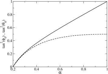
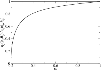
Figure 2: left: $\tan{(\phi_{0})}^{2}$ (straight) and $\tan{(\theta_{0})}^{2}$ (dashed) at the Mott transition as a function of bandwidth ratio $\alpha$; right: Ratio of renormalisation factors $q_{2}/q_{1}$ at the Mott transition as a function of $\alpha$.

As expected, the weight of local states with no electron in the narrow band vanishes for $\alpha\rightarrow\alpha_{\rm c}$. The renormalisation factors $q_{b}$ both vanish proportional to a square-root, $q_{b}\sim\sqrt{U_{c}-U}$, when $U$ approaches $U_{c}$ from below. The ratio $q_{2}/q_{1}$ is finite for $U\rightarrow U_{c}$ and goes to zero proportional to $\sqrt{\alpha-\alpha_{c}}$, see figure 2 (right). Finally, the critical interaction strength $U_{{\rm c}2}=U_{{\rm c}1}$ is given as

$$U_{{\rm c}1}=2|\varepsilon_{0}|f(\phi_{0},\theta_{0})\,\,\,\,\,\,\,\,\,(\alpha>\alpha_{\rm c})\;\;.$$ (35)

Next, we consider the case $\alpha<\alpha_{\rm c}$. For interaction parameters $U_{{\rm c}2}<U<U_{{\rm c}1}$, the electrons in the narrow band are localised and the wide band can be treated as an effective one-band model. This leads us to the critical interaction parameter

$$U_{{\rm c}1}=2|\varepsilon_{0}|f(0,0)=16|\varepsilon_{0}|\,\,\,\,\,\,\,\,\,(\alpha<\alpha_{\rm c})$$ (36)

for the Brinkmann-Rice transition of the wide band. Starting from the Brinkmann-Rice solution for $U<U_{{\rm c}1}$, we can expand the variational energy to leading (i.e. second) order with respect to the three parameters $\{v_{i}\}=\{\phi,\theta,m_{\emptyset}\}$,

$$E=E_{0}+\sum_{i,j=1}^{3}v_{i}\tilde{E}_{i,j}v_{j}\,.$$ (37)

The localisation of the narrow band becomes unstable when the matrix $\tilde{E}$ has negative eigenvalues for physical parameters $v_{i}>0$. This evaluation yields the following expression for the narrow-band critical interaction strength

$$U_{{\rm c}2}=16|\varepsilon|\frac{\alpha}{1-4\alpha}\,\,\,\,\,\,\,\,\,\,(\alpha<\alpha_{\rm c}).$$ (38)

The resulting phase diagram for all $0\leq\alpha\leq 1$ is shown in figure 3.

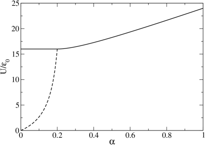
Figure 3: Critical interaction parameters $U_{{\rm c}1}$ (straight) and $U_{{\rm c}2}$ (dashed) as a function of $\alpha$ (see eqs. (35), (36), (38)).

5 The spinless two-band model

As the simplest example for a model with different densities of states we investigate the spinless two-band model. In the half filled case and without spontaneous hybridisation ($\Delta_{0}=0$) the constraints (25) and (3.2) can be solved analytically for this model. The variational energy is then solely a function of $\lambda_{d}$,

$$E_{\rm var}=4\lambda_{d}^{2}\left(1-\frac{\lambda_{d}^{2}}{2}\right)\varepsilon_{0}+\frac{U}{4}\lambda_{d}^{2}\;.$$ (39)

The energy (39) can be minimised analytically. As a result one finds the well known Brinkmann-Rice solution

$$q_{\rm BR} = 1-\left(\frac{U}{U_{\rm c}}\right)^{2}\,,$$ (40)

$$d_{\rm BR} = \frac{1}{4}\left(1-\frac{U}{U_{\rm c}}\right)$$ (41)

for the renormalisation factor $q=\delta_{b,b^{\prime}}q_{b,b^{\prime}}$ and the expectation value of the double occupancy $d=\lambda_{d}^{2}/4$. The Brinkmann-Rice metal insulator transition occurs at the critical value $U=U_{\rm c}\equiv 16|\varepsilon_{0}|$.

For the renormalisation factors $\alpha_{b}$ we set $\alpha_{1}+\alpha_{2}=2$, i.e. the difference of the bandwidths is parametrized by $\Delta\alpha\equiv\alpha_{1}-\alpha_{2}$. Starting from the analytic solution for vanishing hybridisation we can calculate the variational ground state energy to leading order in $\Delta_{0}$,

$$E_{\Delta_{0}}=E_{\rm BR}+C(U,\Delta\alpha)\Delta_{0}^{2}\;.$$ (42)

A spontaneous hybridisation will appear if the coefficient $C$ in (42) is negative. The analytical evaluation leads to the Stoner-type instability criterion

$$\frac{f(\Delta\alpha)}{U_{\rm c}D_{0}(0)}<\frac{U/U_{\rm c}\left(2+U/U_{\rm c}\right)}{2\left(1+U/U_{\rm c}\right)^{2}}\equiv g\left(U/U_{\rm c}\right),$$ (43)

where

$$f(\Delta\alpha)\equiv\frac{\Delta\alpha}{2\rm arcsinh\left(\Delta\alpha/\sqrt{4-\Delta\alpha^{2}}\right)}.$$ (44)

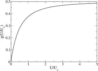
Figure 4: left: $f\left(\Delta\alpha\right)$; right: $g(U/U_{\rm c})$

In figure 4 the function $f(\Delta\alpha)$ and the right hand side of equation (43) are shown as a function of $\Delta\alpha$ and $U$, respectively. As can be seen from this figure the function $f(\Delta\alpha)$ and therefore the left hand side of (43) approach zero for $\Delta\alpha\rightarrow 2$. On the other hand, the right hand side of (43) is positive for all $U>0$. This means that for arbitrary values of $U$ there exist a critical bandwidth difference $\Delta\alpha_{\rm c}$ with $\Delta_{0}>0$ for $\alpha>\alpha_{\rm c}$. Figure 5 (left) shows the phase-diagram for ground states with and without finite hybridisation for different values of the density of states $D_{0}(0)$ at the Fermi-level. Whether or not there is a transition in the large $U$ limit for all values of $\Delta\alpha$ depends on the value of $D_{0}(0)$. This is illustrated in figure 5 (right) where the critical difference $\Delta\alpha_{\rm c}$ for the transition is shown as a function of $D_{0}(0)$ in the limit $U\rightarrow\infty$. Note that a spontaneous hybridisation has already been observed in a Falicov-Kimball model within a mean-field approximation [18]. This is in agreement with our results in the limit $\Delta\alpha\rightarrow 2$.

Figure 5: left:phase diagram of the spinless two-band Hubbard model for different densities of states at the Fermi level $D(0)=0.25,0.2,0.15,0.13,0.125,0.1$ (from the bottom to the top of the figure) right: critical difference $\Delta\alpha_{\rm c}$ in the limit $U\rightarrow\infty$ as a function of $D_{0}(0)$.

In summary, our analytical results on the spinless two-band Hubbard model show that a difference in the bandwidth increases the tendency of the system to exhibit spontaneous hybridisation between the narrow band and the wide band. Mathematically, the reason for this is quite simple. Both, the expectation value of the one-particle energy $\hat{H}_{0}$ and the Coulomb interaction $\hat{H}_{\rm loc}$ are changing quadratically in $\Delta_{0}$. However, in the limit $\Delta\alpha\rightarrow 0$ the energy gain from $\hat{H}_{\rm loc}$ always beats the rise in energy due to $\hat{H}_{0}$. At first glance, one might think that the same behaviour should be observed in the OSMT phase of the two-band model with the only difference that it is not the bare but the effective width of the narrow band that vanishes. As we will discuss in the next section, however, this hypothesis turns out to be incorrect.

6 Hybridisation in the two-band model

In this section we present numerical results for the two-band model with a finite local hybridisation (11). The hybridisation can develop either spontaneously, like in the spinless model (section 5), or it can be caused by a finite hybridisation term in the Hamiltonian. We will discuss both effects separately.

6.1 Spontaneous hybridisation

Figure 6: Renormalisation factors $q_{1}$, $q_{2}$ and hybridisation $2\Delta_{0}$ for $J=0$ and $\alpha=0.15$.

As shown in section 5, a vanishing width of the narrow band can be the driving force for a spontaneous local hybridisation of the wide and the narrow band. In our two-band model, however, the vanishing of the effective bandwidth for $q_{2}\rightarrow 0$ does not have the same effect. This can be seen in figure 6, where we show the results for the renormalisation factors $q_{1}$, $q_{2}$ and the hybridisation $\Delta_{0}$. Unlike in the spinless model, there is not necessarily a finite hybridisation if the effective narrow bandwidth goes to zero for $U\rightarrow U_{{\rm c}2}$. The reason for this differing behaviour is an additional contribution to the one-particle energy of the full two-band model. To leading order in $\Delta_{0}$ there is a third term from the expansion of the narrow-band renormalisation factor

$$q_{2}\approx q_{2}(\Delta_{0}=0)+c\Delta_{0}^{2}\,.$$ (45)

The coefficient $c$ is negative and, multiplied with the negative bare one-particle energy of the narrow band it leads to an increase of the total energy. This contribution to the energy overcompensates the negative term from the Coulomb interaction.

A finite hybridisation $\Delta_{0}$ sets in at larger values of $U$ when the system is already in the OSMT phase, see figure 6. Numerically, it seems as if $\Delta_{0}$ approaches its maximum value $\Delta_{0}^{\rm max}=1/2$ only in the limit $U\rightarrow\infty$.

In all systems with finite values of $J$ that we investigated, we did not find a solution with spontaneous hybridisation. It is more likely, though, that for values of $J$ smaller than some critical parameter $J_{\rm c}$ there is a solution with a finite hybridisation. However, it is difficult to determine this small parameter $J_{\rm c}$ numerically.

6.2 Finite hybridisation in the Hamiltonian

The assumption that there is no hybridisation between the two degenerate bands in the Hamiltonian of our model is quite artificial. In this section we will therefore investigate how the OSMT is affected if we add a hybridisation term of the form

$$\hat{H}_{\rm hyb}=-\tilde{\eta}\sum_{i,\sigma}\hat{c}^{\dagger}_{i1\sigma}\hat{c}_{i2\sigma}+{\rm h.c.}$$ (46)

to our Hamiltonian (2).

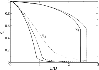
Figure 7: left:expectation value $2\Delta_{0}$ as a function of $U$ for several values of $\tilde{\eta}$; right:Renormalisation factors $q_{1}$, $q_{2}$ for $\alpha=0.15$ and $\tilde{\eta}=0.025D$, $J=0.05U$ (straight), $\tilde{\eta}=0.025D$, $J=0.025U$ (dashed), $\tilde{\eta}=0.05D$, $J=0.025U$ (dotted).

For $J=0$ we find that the OSMT phase is destroyed for any finite value of $\tilde{\eta}$. This is illustrated in figure 7 (left) where we show the expectation value $\Delta_{0}$ as a function of $U$ for several values of $\tilde{\eta}$.

For finite $J$, the behaviour of our model is more ambiguous. As we have seen before, a finite $J$ stabilizes the OSMT phase whereas a finite $\tilde{\eta}$ tends to destroy it. Therefore, it depends on the ratio of both quantities whether or not an OSMT is found. Figure 7 (right) shows the renormalisation factors $q_{b}$ for different values of $J$ and $\tilde{\eta}$. For $J=0.025U$ and $\tilde{\eta}=0.05D$ the OSMT is completely suppressed. This is still the case for the smaller value $\tilde{\eta}=0.025D$, although the narrow band factor $q_{2}$ is already quite small in the region of $U$ parameters where it would be zero for $\tilde{\eta}=0$. Finally, for larger values $J=0.05U$ an OSMT phase is restored for interaction parameters $U>U_{{\rm c}2}$ where $U_{{\rm c}2}$ is larger then the corresponding value for $\tilde{\eta}=0$.

In summary, our numerical calculations show that appearance and disappearance of an OSMT results from a subtle interplay of the local exchange interaction $J$ and the local hybridisation $\tilde{\eta}$.

7 Summary

In this work we have investigated the orbital selective Mott transition (OSMT) in two-band Hubbard models with different densities of states by means of the Gutzwiller variational theory. We were particularly interested in the question how the OSMT is modified when we allow for a finite local hybridisation between the wide band and the narrow band. In the two-band model without spin-degrees of freedom there always is a spontaneous hybridisation if the narrow bandwidth goes to zero. However, we did not find such a behaviour in the full two-band model. There, spontaneous hybridisation was only seen for vanishing local exchange interaction, $J=0$, and for Coulomb parameters $U$ larger then the critical parameter at which the electrons in the narrow band localise. By adding a local hybridisation term $\sim\tilde{\eta}$ to the Hamiltonian, the phase diagram becomes more involved. Whether or not an OSMT takes place depends on the relative strength of $J$ and $\tilde{\eta}$. The exchange interaction $J$ tends to stabilise the OSMT phase, whereas the hybridisation $\tilde{\eta}$ tends to destroy it.

References

- [1] Liebsch A 2003, Europhysics Letters 63 97
- [2] Liebsch A 2003, Phys. Rev. Lett. 91 226401
- [3] Liebsch A 2004, Phys. Rev. B 70 165103
- [4] Koga A, Kawakami N, Rice T, and Sigrist M 2004, Phys. Rev. Lett. 92 216402
- [5] Koga A, Kawakami N, Rice T, and Sigrist M 2005, Phys. Rev. B 72 045128
- [6] Knecht C, Blümer N, and van Dongen P G J 2005 Phys. Rev. B 72, 081103
- [7] de Medici L, Georges A, and Biermann S 2005 Phys. Rev. B 72 205124
- [8] Arita R, and Held K 2005 Phys. Rev. B 72 201102
- [9] Ferrero M, Becca F, Fabrizio M, and Capone M 2005 Phys. Rev. B 72 205126
- [10] Dai X, Kotliar G, and Fang Z (unpublished)
- [11] Gutzwiller M C 1963 Phys. Rev. Lett. 10 159
- [12] Vollhardt D 1984 Rev. Mod. Phys. 56 99
- [13] Bünemann J 1998 Eur. Phys. J. B 4 29
- [14] Gebhard F 1990 Phys. Rev. B 41 9452
- [15] Bünemann J, Weber W, and Gebhard F 1998
- [16] Bünemann J, Gebhard F, and Weber W 2005 Frontiers in Magnetic Materials, ed A Narlikar (Berlin: Springer)
- [17] Bünemann J, Gebhard F, Radnóczi K, and Fazekas K 2005 J. Phys. Cond. Matt. 17 3807
- [18] Czycholl G 1999 Phys. Rev. B 59 2642.