Orbital Solution & Fundamental Parameters of $\sigma$ Scorpii

Abstract

The first orbital solution for the spectroscopic pair in the multiple star system $\sigma$ Scorpii, determined from measurements with the Sydney University Stellar Interferometer (SUSI), is presented. The primary component is of $\beta$ Cephei variable type and has been one of the most intensively studied examples of its class. The orbital solution, when combined with radial velocity results found in the literature, yields a distance of $174^{+23}_{-18}$ pc, which is consistent with, but more accurate than the Hipparcos value. For the primary component we determine $18.4\pm 5.4$ M_☉, $-4.12\pm 0.34$  mag and $12.7\pm 1.8$ R_☉ for the mass, absolute visual magnitude and radius respectively. A B1 dwarf spectral type and luminosity class for the secondary is proposed from the mass determination of $11.9\pm 3.1$ M_☉ and the estimated system age of 10 Myr.

1 Introduction

The class of variable stars with $\beta$ Cephei as the prototype consists of massive, nonsupergiant stars whose low-order pressure and gravity mode pulsations result in light, radial and/or line profile variations (Stankov & Handler, 2005). In the most recent catalogue of $\beta$ Cephei type variables, the 93 confirmed members have periods of strongest pulsation (some members display multi-mode pulsation behaviour) ranging from 1–8 hours and are of spectral type B0–B3 (Stankov & Handler, 2005).

Approximately 14% of the catalogued $\beta$ Cephei stars are located in multiple star systems and therefore, with sufficient observational data, component masses can be determined for comparison with those estimated from theory. Indeed this has been achieved in the cases of $\alpha$ Virginis (Herbison-Evans et al., 1971), $\beta$ Centauri (Davis et al. 2005; Ausseloos et al. 2006) and $\lambda$ Scorpii (Tango et al., 2006) by combining the results of spectroscopic and interferometric analysis. Recently, analysis of the eclipsing binary HD 92024 has also yielded the mass determination of the $\beta$ Cephei primary (Freyhammer et al., 2005). This last result is of particular interest as Freyhammer et al. (2005) note that the HD 92024 primary component spectrum closely resembles that of $\sigma$ Sco.

As a ‘classical’ member (Lesh & Aizenman, 1978) of the $\beta$ Cephei variable type stars, $\sigma$ Sco (HR 6084, HD 147165) has been one of the most intensively studied examples of this class and has also been used as a photometric standard (Vijapurkar & Drilling, 1993). Lutz & Lutz (1977) classified the system as a binary with B2 IV + B9.5 V components separated by 20″  on the sky and a visual magnitude difference of 5.31 mag. Speckle interferometry, lunar occultations and spectroscopy have since shown that the B2 IV component is in fact three stars – a double-lined spectroscopic pair and a 2.2  mag fainter B7 tertiary, 0.4″distant from the spectroscopic pair (Beavers & Cook 1980; Evans et al. 1986; Mathias et al. 1991). The primary component has been identified as a $\beta$ Cephei type pulsator and has a classification of B1 III. Therefore the system, as it stands in the literature, is quadruple: a spectroscopic pair, a tertiary component, and the fourth star is the fainter component in the visual common proper motion pair ADS 10009 (Pigulski, 1992).

The atmosphere of the $\beta$ Cephei component was analysed by Vander Linden & Butler (1988), who gave an effective temperature of $26\,150\pm 1\,070$ K with a pulsation cycle variation of $4\,000\pm 2\,000$ K. These authors also gave an excellent synopsis of early radial velocity and line profile studies of the spectroscopic pair. Mathias et al. (1991) used a double-shock wave propagating in the stellar atmosphere to explain the observed stillstand in the radial velocity curves of the 656.3 nm H $\alpha$, 658.3 nm C II and 455.3 nm Si III lines (a period of about an hour wherein the radial velocity remains relatively constant). The double-shock wave model was also successful in describing similar characteristics of two other $\beta$ Cephei stars: BW Vul and 12 Lac (Mathias et al., 1992). The study of Mathias et al. (1991) was also the first to detect the spectral lines of the companion in the spectroscopic pair. However, neither the spectral type, luminosity class nor an estimate of the flux ratio (secondary/primary) was presented in Mathias et al. (1991). $\sigma$ Sco also exhibits a conspicuous Van Hoof effect – a small phase lag of the radial velocity of the hydrogen lines relative to that of all other lines (Vander Linden & Butler 1988; Mathias et al. 1991).

The most recent analyses of the spectroscopic pair by Mathias et al. (1991), Chapellier & Valtier (1992) and Pigulski (1992) have produced orbital periods of 33.012, 33.011 and 33.012 days respectively. Pigulski (1992) has also concluded that the variations in the main pulsation period (increase in the first half of the 1900s, decrease after 1960, and again an increase from about 1984) are due to a combination of evolutionary and light-time effects.

Hereafter, the following naming convention will be followed. The primary and secondary refer to the spectroscopic pair. The tertiary refers to the star that is approximately 2.2 mag fainter and separated by 0.4″  from the spectroscopic pair. The fourth and final star will be referred to as the distant companion. The term $\sigma$ Sco will refer to the spectroscopic pair unless explicitly stated otherwise.

In Section 3 we provide the first complete orbital solution for $\sigma$ Sco determined by long-baseline optical interferometry. In combination with the only double-lined radial velocity measurements, the distance, spatial scale, mass and age of the components are quantified and compared to previous estimates in Section 4. The details of our observations and a description of the parameter fitting procedure are described in Sections 2 and 3 respectively.

2 Observations and Data Reduction

Measurements of the squared visibility (i.e. the squared modulus of the normalised complex visibility) or $V^{2}$ were completed on a total of 31 nights using the Sydney University Stellar Interferometer (SUSI, Davis et al. 1999). Interference fringes were recorded with the red beam-combining system using a filter with centre wavelength and full-width half-maximum of 700 nm and 80 nm respectively. This system was outlined by Tuthill et al. (2004) and is to be described in greater detail by Davis et al. (in preparation).

Table 1: Adopted parameters of reference stars used during observations. The angular diameters (and associated error) were estimated from an intrinsic colour interpolation (and spread in data) of measurements made with the Narrabri Stellar Intensity Interferometer (Hanbury Brown et al., 1974).

HR	Name	Spectral	V	UD Diameter	Separation
		Type		(mas)	from $\sigma$ Sco
5928	$\rho$ Sco	B2IV/V	3.88	$0.25\pm 0.03$	6$\aas@@fstack{\circ}$50
5993	$\omega^{1}$ Sco	B1Vp	3.96	$0.26\pm 0.04$	5$\aas@@fstack{\circ}$93
6153	$\omega$ Oph	A7Vp	4.45	$0.50\pm 0.02$	4$\aas@@fstack{\circ}$83
6165	$\tau$ Sco	B0V	2.82	$0.31\pm 0.06$	4$\aas@@fstack{\circ}$20

The observations and data reduction followed the procedure outlined by North et al. (2007) using the adopted stellar parameters of the calibrator stars given in Table 1. A total of 262 estimations of $V^{2}$ were available for analysis (not including two observations that were removed due to possible tertiary contamination, Section 3.1) as summarised in Table 2.

Table 2: Summary of observational data. The night of the observation is given in columns 1 and 2 as a calendar date and a mean MJD. Column 3 is the mean orbital phase calculated from the values in Table 4. The baseline and the mean projected baseline (in units of metres) are given in columns 4 and 5 respectively. Reference stars and the the number of squared visibility measures for a night are listed in the last two columns.

Date	MJD	Phase	Nominal	Projected	Reference	# V2
			Baseline	Baseline	Stars
2005 May 20	53510.64	0.121	80	79.80	$\tau$ Sco, $\rho$ Sco, $\omega$ Oph	4
2005 May 24	53514.58	0.240	80	79.78	$\tau$ Sco, $\rho$ Sco, $\omega$ Oph	10
2005 May 25	53515.59	0.271	80	79.74	$\tau$ Sco, $\rho$ Sco	4
2005 July 19	53570.46	0.933	80	79.81	$\tau$ Sco, $\rho$ Sco, $\omega$ Oph	10
2005 July 20	53571.43	0.962	80	79.78	$\tau$ Sco, $\rho$ Sco, $\omega^{1}$ Sco	11
2005 August 08	53590.46	0.539	80	79.89	$\tau$ Sco, $\omega^{1}$ Sco	11
2005 August 11	53593.40	0.638	80	79.80	$\tau$ Sco, $\omega^{1}$ Sco	8
2005 August 13	53595.43	0.689	80	79.85	$\tau$ Sco, $\omega^{1}$ Sco	10
2005 August 16	53598.37	0.778	80	79.73	$\tau$ Sco, $\omega^{1}$ Sco	2
2006 June 15	53901.55	0.963	80	79.76	$\tau$ Sco, $\rho$ Sco, $\omega^{1}$ Sco	3
2006 June 16	53902.56	0.993	80	79.82	$\tau$ Sco, $\rho$ Sco	9
2006 June 17	53903.50	0.022	80	79.83	$\tau$ Sco, $\rho$ Sco	12
2006 June 18	53904.54	0.053	80	79.83	$\tau$ Sco	15
2006 June 24	53910.52	0.234	80	79.80	$\tau$ Sco	11
2006 June 25	53911.48	0.264	80	79.78	$\tau$ Sco	8
2006 June 26	53912.50	0.293	80	79.83	$\tau$ Sco	3
2006 June 27	53913.53	0.326	80	79.88	$\tau$ Sco	8
2006 June 28	53914.48	0.354	80	79.83	$\tau$ Sco	12
2006 July 18	53934.40	0.958	80	79.82	$\tau$ Sco	2
2006 July 19	53935.43	0.989	80	79.81	$\tau$ Sco	11
2006 July 25	53941.41	0.170	80	79.78	$\tau$ Sco	8
2006 August 01	53948.41	0.382	80	79.80	$\tau$ Sco, $\rho$ Sco	12
2006 August 03	53950.40	0.442	80	79.77	$\tau$ Sco, $\rho$ Sco, $\omega^{1}$ Sco	8
2006 August 04	53951.37	0.472	40	39.88	$\tau$ Sco	4
2006 August 07	53954.42	0.564	40	39.91	$\tau$ Sco, $\rho$ Sco, $\omega^{1}$ Sco	13
2006 August 08	53955.45	0.596	30	29.94	$\tau$ Sco, $\rho$ Sco, $\omega^{1}$ Sco	12
2006 August 09	53956.42	0.625	30	29.93	$\tau$ Sco, $\rho$ Sco, $\omega^{1}$ Sco	12
2006 August 10	53957.42	0.655	30	29.94	$\tau$ Sco, $\rho$ Sco, $\omega^{1}$ Sco	12
2006 August 22	53969.40	0.018	55	54.92	$\tau$ Sco	6
2006 August 26	53973.41	0.140	55	54.95	$\tau$ Sco	6
2006 August 27	53974.38	0.169	30	29.93	$\tau$ Sco, $\rho$ Sco, $\omega^{1}$ Sco	5

3 Orbital Solution

The theoretical response of a two aperture interferometer to the combined light of a binary star is given by (Hanbury Brown et al., 1970)

$$V^{2}=\frac{V_{1}^{2}+\beta^{2}V_{2}^{2}+2\beta|V_{1}||V_{2}|\cos(2\pi\mn@boldsymbol{b}\cdot\mn@boldsymbol{\rho}/\lambda)}{(1+\beta)^{2}},$$ (1)

where $\beta<1$ is the brightness ratio of the two stars in the observed bandpass and $V_{1}$, $V_{2}$ are the visibilities of the primary and secondary respectively. In the simplest case, stars can be modeled by a disc of uniform brightness with angular diameter $\theta$ (see Section 4.3 for the effects of limb-darkenening). The component visibilities in equation (1) are then given by

$$V=\frac{2J_{1}(\pi|\mn@boldsymbol{b}|\theta/\lambda)}{\pi|\mn@boldsymbol{b}|\theta/\lambda},$$ (2)

where $J_{1}$ is a first order Bessel function. The angular separation vector of the secondary with respect to the primary is given by $\mn@boldsymbol{\rho}$ (measured east from north), $\mn@boldsymbol{b}$ is the interferometer baseline vector projected onto the plane of the sky and $\lambda$ is the centre observing wavelength. The observed $V^{2}$ will vary throughout the night due to the orbital motion of the binary and Earth rotation of $\mn@boldsymbol{b}$. The Keplerian orbit of a binary star, i.e. $\mn@boldsymbol{\rho}$ as a function of time, can be parameterized with seven elements: the period $P$, eccentricity $e$, the longitude of periastron $\omega$, epoch of periastron $T_{0}$, semi-major axis $a$, the longitude of ascending node $\Omega$ and the inclination $i$. When using two-aperture optical interferometry, the phase of the complex visibility is lost and hence, $\Omega$ and $\omega$ have an ambiguity of 180°. This is a direct result of the fact that component identities cannot be determined. Measurements of radial velocity can be used to remove the ambiguity of $\omega$ but that of $\Omega$ remains.

3.1 Effects of the Tertiary and Distant Companion

The presence of a third or fourth component can greatly complicate analysis of interferometric data. The distant component is too far away and too faint to affect the interferometric data and can be neglected. Therefore, an investigation into the effects of the tertiary star was conducted to validate the data and aid the final analysis.

Firstly, the mean location of the tertiary, relative to the spectroscopic pair, was estimated by fitting a simple smoothed curve trajectory to the published vector separations. The literature vector separations are given in Table 3 and are shown with the fitted curve in Fig. 1. The estimated vector separation for the mean observing date of the SUSI observations (B2006.357) is $\rho=486$ mas and $\theta=238^{\circ}$ where $\rho$ and $\theta$ are the magnitude and angle of the separation vector. The magnitude difference of the tertiary with respect to the combined spectroscopic pair irradiance is approximately $2.23\pm 0.18$ mag (mean and standard deviation of the values from Hartkopf et al. 2006 adjusted to our passband). Given the estimated separation (which is within SUSI’s field-of-view), the irradiance of the tertiary star will be detected by SUSI and must be included in the analysis.

Table 3: Literature vector separations of the tertiary measured with respect to the spectroscopic pair. Methods are O: Occultation; S: Speckle; H: Hipparcos; C: Coronograph

Besselian	$\rho$	$\theta$	Method: Reference
Year	(mas)	(deg)
1972.556	322	296.8	O: Evans et al. (1986)
1976.471	326	291.8	S: Morgan et al. (1978)
1977.4868	353	285.4	S: McAlister (1979)
1980.4792	367	277.4	S: McAlister et al. (1983)
1980.4819	367	277.9	S: McAlister et al. (1983)
1981.4567	372	275.2	S: McAlister et al. (1984)
1981.4704	369	277.1	S: McAlister et al. (1984)
1981.4730	369	275.6	S: McAlister et al. (1984)
1983.4254	377	272.6	S: McAlister et al. (1987)
1984.3783	384	272.3	S: McAlister et al. (1987)
1986.243	392	268.5	O: Evans et al. (1986)
1987.2726	407	264.5	S: McAlister et al. (1989)
1989.2275	416	261.4	S: McAlister et al. (1990)
1989.3038	414	261.4	S: McAlister et al. (1990)
1991.3140	428	258	H: ESA (1997)
1993.3424	430	256	S: Miura et al. (1995)
1994.3509	441	253	S: Mason (1996)
1997.2252	443	249.3	S: Horch et al. (1999)
1997.5174	465	242.9	S: Horch et al. (1999)
1997.5174	456	249.5	S: Horch et al. (1999)
1997.6157	447	248.8	S: Horch et al. (1999)
2000.3996	469	244.4	C: Shatsky & Tokovinin (2002)

Figure 1: Literature vector separations of the tertiary measured with respect to the spectroscopic pair. Lunar occultations are given as triangles, speckle interferometry as diamonds, Hipparcos results as a square and the coronographic measurement as a cross. The plus symbol represents the location of the spectroscopic pair. The dotted line is a simple smooth trajectory fit to the data and the asterisk is the estimated mean position of the tertiary during SUSI observations.

The offset of the tertiary fringe packet in delay space, $D$, was calculated using

$$D=|{\bf b}|\rho\cos\left(\eta-\theta\right),$$ (3)

assuming that the spectroscopic pair’s fringe packet is located at the phase centre of SUSI. $|{\bf b}|$ and $\eta$ are the projected baseline length and position angle respectively. It was found that only two observations had an offset within the centre half of the 140 $\mu$m observing scan. For approximately 72% of the observations, the offset was sufficiently large to place the tertiary fringe packet entirely outside the observing scan. However, the SUSI data reduction pipeline windows the recorded scan about the detected peak fringe location (Ireland, 2005). Therefore, the tertiary fringe packet will not be within the ‘data window’ and should not affect the calculation of $V^{2}$ if both

1. the offset is sufficiently large, and

2. the fringe packet of the spectroscopic pair has a greater amplitude than that of the tertiary (i.e. avoid the system ‘locking’ onto the tertiary).

The first condition can easily be satisfied by the removal of all observations with an offset less than 30 $\mu$m – the outer quarter of a scan (beyond the edge of the window function). Hence, the two data points that were found within the centre half of the fringe scan were rejected from the analysis. The second condition may not be satisfied when the primary and secondary fringe packets destructively interfere; i.e. at a minimum in the modulation of $V^{2}$ there is the possibility of mistakenly measuring the interference pattern of the tertiary. Assuming the primary and secondary fringe packet destructive interference is absolute and the tertiary is completely unresolved, then the expected $V^{2}\la 0.013$ will be due to the tertiary alone. As this is below the $V^{2}$ detection limit of SUSI, we can neglect such cases. Hence all remaining observations of $\sigma$ Sco now satisfy both conditions. The SUSI data pipeline will nevertheless be affected by the incoherent flux from the tertiary component. The required adjustment to the fitted squared-visibility model is given in the next section.

3.2 Fitting Procedure and Uncertainty Estimation

The validity of equation (1) is (strictly) only for observations of binary stars made with very narrow bandwidths. For real detection systems wide bandwidth effects can reduce the observed $V^{2}$ and for the scanning detection system of SUSI, the equivalent to equation (1) giving $V^{2}$ for a binary star for the case of a wide spectral bandwidth is (North et al., 2007):

$$V^{2}=\frac{V_{1}^{2}+\beta^{2}V_{2}^{2}+2\beta r(\psi)|V_{1}||V_{2}|\cos(\psi)}{(1+\beta)^{2}},$$ (4)

where

$$r(\psi)=\exp\left[\frac{-\Delta\lambda^{2}}{\lambda_{0}^{2}}\frac{\psi^{2}}{32\ln 2}\right].$$ (5)

The spectral response is approximated as a Gaussian of centre wavelength $\lambda_{0}$ with full-width half-maximum $\Delta\lambda$. The term $r(\psi)$ corresponds to the autocorrelation of the Gaussian envelope of the interference pattern and $\psi=2\pi\mn@boldsymbol{b}\cdot\mn@boldsymbol{\rho}/\lambda_{0}$ is defined for convenience.

The measures of $V^{2}$ are contaminated by the irradiance of the tertiary star (Section 3.1) such that equation (4) is no longer applicable. The brightness ratio $I_{3}$ of the tertiary/(primary + secondary) is approximately $I_{3}\simeq 0.128\pm 0.023$ (Section 3.1). Adjusting equation (4) for the contamination of the tertiary we obtain

$$|V|^{2}=\frac{V_{1}^{2}+\beta^{2}V_{2}^{2}+2\beta|V_{1}||V_{2}|r(\psi)\cos(\psi)}{[(1+I_{3})(1+\beta)]^{2}}.$$ (6)

The term, $I_{3}$, reduces the observed $V^{2}$ and hence the effect the tertiary component has on the calculated $V^{2}$ of the spectroscopic pair is considered an extra incoherent source. The addition of this term will mainly affect the fitted component angular diameters and brightness ratio, leaving the orbital parameters relatively unaffected. As $\Delta\lambda$ and $I_{3}$ approach zero, i.e. narrow bandwidth observations of a simple binary star, then equation (6) reduces to equation (1).

Initial values of the inclination and position angle of the ascending node were found by a coarse grid search of parameter space. The remaining orbital parameters were limited to within three standard deviations of the values given by Mathias et al. (1991). The inital angular diameter of the primary star was estimated from the Hipparcos distance and spectral type characteristics found in the literature (Cox 2000). By physical arguments and inspection of the measured $V^{2}$ values, the secondary’s angular diameter and brightness ratio were limited to the ranges 0.2–0.6 mas and 0.2–0.8 respectively.

The final estimation of parameters was completed using $\chi^{2}$ minimization as implemented by the Levenberg-Marquardt method to fit equation (6) to the observed values of $V^{2}$. When finding the minimum of the $\chi^{2}$ manifold, the inverse of the covariance matrix is calculated by the non-linear fitting program. The formal uncertainties of the fitted parameters are derived from the diagonal elements of this covariance matrix. As the visibility measurement errors may not strictly conform to a normal distribution and equation (6) is non-linear, the formal uncertainties may be underestimates. Following the approach of North et al. (2007), three uncertainty estimation methods were adopted to confirm the accuracy of the values derived from the covariance matrix. These methods: Monte Carlo, bootstrap and Markov chain Monte Carlo (MCMC) simulations are described by North et al. (2007) and references therein.

3.3 Results

Table 4: Orbital and physical parameters of $\sigma$ Sco as found with SUSI and from the literature. The periods from the literature have been converted to MJD and/or adjusted to the same epoch. Note that the difference between the Heliocentric Julian Day (HJD) and a Julian Day is less than ten minutes which is much smaller than the uncertainties.

Parameter	Unit	SUSI	Mathias et al. (1991)	Pigulski (1992)
$P$	days	$33.010\pm 0.002$	$33.012\pm 0.002$	$33.012$
$e$		$0.3220\pm 0.0012$	$0.44\pm 0.11$	$0.40\pm 0.04$
$T_{0}$	MJD	$34889.0\pm 1.0$	$34888.9\pm 0.7^{b}$	$34888.0\pm 0.4^{c}$
$\omega$	deg	$283\pm 5^{d}$	$299.1\pm 10.0$	$287\pm 6$
$a^{\prime\prime}$	mas	$3.62\pm 0.06$	-	-
$\Omega$	deg	$104\pm 5$	-	-
$i$	deg	$158.2\pm 2.3$	-	-
$\theta_{1}$	mas	$0.67\pm 0.03$	-	-
$\theta_{2}$	mas	$0.34\pm 0.04^{a}$	-	-
$\beta$		$0.48\pm 0.02$	-	-

^a Adopted parameters; ^b HJD-2400000.5; ^c 498 $\times$ 33.012d added; ^d Ambiguity of 180°.

Figure 2: Data from the nights of 2005 Aug 08 (top-left), 2006 Aug 08 (bottom-left), 2006 Jun 24 (top-right) and 2006 Jun 28 (bottom-right) where each data point represents a measure of $V^{2}$ with the associated formal error. The values of Table 4 have been been used to show the fitted model as a solid line.

From preliminary analysis, a classification of B1 V was adopted for the secondary (see Section 4.4) and its angular diameter was assumed to be $0.34\pm 0.04$ mas (i.e. a radius of 6.4 R_☉ – with a 12 per cent uncertainty – at the distance obtained from the dynamical parallax). The three parameters $\theta_{1}$, $\theta_{2}$ and $\beta$ are coupled and hence a change in one will affect the other two without significantly changing the orbital parameters.

The best-fitting values of the model parameters are given in Table 4 and four nights data are shown in Fig. 2 with the predicted $V^{2}$ model overlaid as the solid curve. The projected orbit on the plane of the sky is shown in Fig 3.

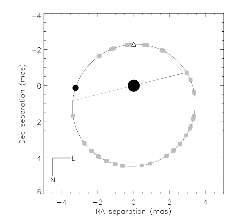
Figure 3: The relative orbit (solid line) of the secondary about the $\beta$ Cephei star projected on the plane of the sky. The dotted line is the line-of-nodes, the open triangle signifies periastron and the grey squares are parts of the orbit that were observed with SUSI. The stellar components (filled circles) are drawn to scale using the values of Table 4. The secondary is shown at an orbital phase of 0.85.

The reduced $\chi^{2}$ of the fit was 3.58, implying that the measurement errors are underestimated by a factor of 1.89. Two possible effects were investigated. Firstly, the seeing conditions during some observations were poor and then only the brightest calibrator could be used, resulting in data of lower quality than on other nights. While a non-linear seeing correction (Ireland, 2006) was applied to all data as part of the data reduction, there could be some residual atmospheric effects. Secondly, the primary star, being of $\beta$ Cephei pulsator type, varies in diameter, temperature and apparent brightness. These properties will also affect the results of fitting equation (6) to the data and contribute to the somewhat large value of reduced $\chi^{2}$ and non-Gaussian parameter uncertainty distributions (discussed further below). However the quality and resolution of the SUSI data combined with the uncertainty in the literature values does not justify a more complicated model that includes the intrinsic variability. Furthermore, the number and time base of $V^{2}$ measures is sufficient to average out any effects from the intrinsic variability of the primary. Hence, the angular diameter of the primary, along with the component brightness ratio, are treated as mean values by equation (6).

The three different uncertainty estimation techniques (described in Section 3.2) produced distributions of each free model parameter similar in appearance and approximately centred on the best-fitting values. The Monte Carlo and bootstrap methods were set to each generate $10^{3}$ synthetic data sets while the MCMC simulations completed $10^{7}$ iterations. The shape of the likelihood functions of the semi-major axis, eccentricity, inclination, uniform disc angular diameters and the brightness ratio were Gaussian in appearance. The Probability Density Functions produced by the MCMC simulation for the remaining (free) model parameters were slightly non-Gaussian, most likely due to the intrinsic pulsations of the primary. Even though some model parameters produced (weakly) non-Gaussian distributions, the uncertainty values quoted in Table 4 are the standard deviations. As the MCMC simulation includes the uncertainties in the tertiary incoherent flux and angular diameter of the secondary, the values it produced form the basis of the final parameter uncertainties given in Table 4 because we believe they are the most realistic estimates of parameter uncertainties for our data set.

The orbital parameters found by the analyses of Mathias et al. (1991) and Pigulski (1992), together with the final values determined from the SUSI data, are given in Table 4. The values for the period and time of periastron passage are all in excellent agreement. There is some disagreement among the two remaining orbital parameters when considering the quoted uncertainties. However, all values are consistent at the two standard deviation level. The analysis of Mathias et al. (1991) is considered to be the most up-to-date due to the detection of the secondary spectral lines and the inclusion of the most recent (published) data. Therefore, comparing only the SUSI and the Mathias et al. (1991) results all parameters are consistent at the 1.1 standard deviation level.

4 System and Physical Parameters

Mathias et al. (1991) contains the only published semi-amplitudes of both the primary and secondary components. The small discrepancy between the SUSI and Mathias et al. (1991) eccentricity and longitude of periastron passage may affect the estimation of those physical parameters obtained by the combination of interferometric and spectroscopic results. We note, however, that the inclination is close to 180°and consequently, the uncertainty in $\sin i$ will dominate the error budget (see for example Section 4.1).

4.1 Distance

The calculation of the dynamical parallax,

$$\pi_{d}=\frac{a\arcsec}{(a_{1}+a_{2})},$$ (7)

requires the semi-major axis of the relative orbit in both linear units (i.e. AU) and angular units. Using the interferometric orbital values and the component semi-amplitudes $K_{1}=31.9\pm 1.3$ kms^-1 & $K_{2}=49.3\pm 7.3$ kms^-1(Mathias et al., 1991), the semi-major axes of the component orbits were calculated (in km) using

$$a_{1,2}=\frac{43200K_{1,2}P\sqrt{1-e^{2}}}{\pi\sin i}.$$ (8)

These values are given in Table 5 in units of AU. Combining these values of $a_{1}$ and $a_{2}$ with the angular semi-major axis of the relative orbit in Table 4, the dynamical parallax was found to be $\pi_{d}=5.76\pm 0.68$ mas. The 12% uncertainty in the dynamical parallax is dominated by the contribution of the inclination – the uncertainty in $\sin i$ is 11%.

The distance to the system is therefore $174^{+23}_{-18}$ pc, which is consistent within uncertainties with the Hipparcos value of $225^{+50}_{-35}$ pc. An analysis of the Hipparcos data by de Bruijne (1999) produced a secular parallax of $\pi_{\it sec}=5.27\pm 0.48$ mas (or a distance of $190^{+19}_{-16}$ pc) with which the dynamical parallax (and consequent distance) is in good agreement.

The members of nearby OB associations have been determined by de Zeeuw et al. (1999) from Hipparcos proper motion and parallax measurements. They concluded that $\sigma$ Sco is a secure member of the Upper Scorpius (US) subgroup within the Sco OB2 association with a membership probability of 94%. Using fig. 5 of de Zeeuw et al. 1999, the mean US parallax is 6.9 mas with an estimated uncertainty of about 1.5 mas (de Zeeuw et al. 1999 give a ‘spread’ value of 1.6 mas). Therefore the dynamical parallax positions $\sigma$ Sco closer to the centre of US compared to Hipparcos and hence strengthens membership probability to the Upper Scorpius subgroup.

Table 5: Physical parameters of $\sigma$ Sco. The middle and bottom panels are the values for the primary and secondary respectively.

Parameter	Unit	This Work	Literature	Reference
$a_{1}$	AU	$0.25\pm 0.03$	-	-
$a_{2}$	AU	$0.38\pm 0.07$	-	-
$\pi$	mas	$5.76\pm 0.68$	$4.44\pm 0.81$	ESA (1997)
	mas		$5.27\pm 0.48$	de Bruijne (1999)
distance	pc	$174^{+23}_{-18}$	$225^{+50}_{-35}$	ESA (1997)
			$190^{+19}_{-16}$	de Bruijne (1999)
age	Myr	10	5–14	Brown (1998)
			5	Preibisch et al. (2002)
${\cal M}$(B1 III)	M☉	$18.4\pm 5.4$	-	-
$M_{V}$(B1 III)	mag	$-4.12\pm 0.34$	-	-
$L$(B1 III)	L☉	$(2.9\pm 0.8)\times 10^{4}$	-	-
$R$(B1 III)	R☉	$12.7\pm 1.8$	-	-
${\cal M}$(B1 V)	M☉	$11.9\pm 3.1$	-	-
$M_{V}$(B1 V)	mag	$-3.32\pm 0.34$	-	-
$L$(B1 V)	L☉	$(1.6\pm 0.4)\times 10^{4}$	-	-

4.2 Component Masses

The mass of the primary and secondary can be extracted from the orbital solution by combining Kepler’s third law,

$${\cal M}_{1}+{\cal M}_{2}=\frac{(a_{1}+a_{2})^{3}}{P^{2}},$$ (9)

and the ratio of the component semi-major axes about the centre-of-gravity,

$$\frac{{\cal M}_{1}}{{\cal M}_{2}}=\frac{a_{2}}{a_{1}}.$$ (10)

The calculated masses are in solar units when the semi-major axes are given in astronomical units and the period in years. Using the values determined in Sections 3.3 and 4.1 the primary and secondary star star masses were found to be $18.4\pm 5.4$ M_☉ and $11.9\pm 3.1$ M_☉ respectively. Once again the uncertainty in the mass is dominated by the contribution of the inclination (propagated from the distance determination).

The expected mass of a B1 III star is $17.4$ M_☉ (interpolated from values in Schmidt-Kaler 1982), while the analysis of HD92024 (a B1 III $\beta$ Cephei star with a nearly identical spectrum) by Freyhammer et al. (2005) produced $15^{+3}_{-4}$ M_☉. Our determination of the primary star’s mass in $\sigma$ Sco is in complete agreement with these results. The mass of the primary is larger than the majority of members in the catalogue of Galactic $\beta$ Cephei stars (Stankov & Handler, 2005) where a mass of 12 M_☉ is the norm. The uncertainty in the mass is large, precluding the conclusion that the $\beta$ Cephei component in $\sigma$ Sco is one of the most massive examples of this type of pulsating star.

4.3 $\beta$ Cephei Component Radius

The analysis of the interferometric data yielded the uniform disc angular diameter of the primary component. However, real stars are limb-darkened and corrections are required to find the ‘true’ angular diameter from the uniform disc value. These corrections are discussed (and tabulated) in Davis et al. (2000) and are dependent on the star’s effective temperature, surface gravity, chemical composition and the wavelength at which the uniform disc diameter was determined. Assuming solar chemical composition, for $T_{\mathrm{eff}}=26\,150$ K and $\log g=3.85$ (Vander Linden & Butler, 1988) at an observing wavelength of 700 nm, the limb-darkening correction factor given in Davis et al. (2000) is 1.018 for the primary star. Using the dynamical parallax, the radius can now be estimated to be $12.7\pm 1.8$ R_☉, compatible with a B1 III star (interpolated) from Schmidt-Kaler (1982) and the analysis of the similar star HD92024 by Freyhammer et al. (2005).

4.4 Secondary Component

Even though Mathias et al. (1991) detected spectral features of the secondary star, no estimation of its spectral type or luminosity class appears in the literature.

Initial analysis of the interferometric data included the secondary angular diameter as a fitting parameter and a uniform disc radius of $11$ R_☉ was determined (but poorly constrained). Interpolating spectral type calibration tables in Schmidt-Kaler (1982), stellar types B1 V & B3 III had a mass that was consistent with that of the secondary (Section 4.2). However, the fitted uniform disc radius was too large for a B1 dwarf star ($6.4$ R_☉) but was in accord for a B3 giant ($10.8$ R_☉). On the other hand, single-star evolutionary tracks (Section 4.6) predict vastly different ages for the two components and produce a more evolved state for a B3 giant secondary. Therefore a B1 dwarf classification was adopted and the interferometric data was reanalysed with the additional constraints on the likely radius of the secondary taken into consideration. The results with this new fitting produced plausible values (absolute magnitudes and primary component radius more in line with literature calibrations, and similar ages) and without any significant change in the orbital parameters or quality of the model-fit.

Therefore, evolutionary tracks and the mass determined from the combination of interferometric and spectroscopic results imply a classification of B1 V for the secondary. An approximate effective temperature of $T_{\mathrm{eff}}=25\,400\pm 2\,000$ K (Lang, 1991) is henceforth adopted for the secondary component.

4.5 Component Magnitudes

The absolute visual magnitude of the system can be determined from the distance and the apparent visual magnitude. The mean and standard deviation of extinction values found in the literature are $A_{V}=1.23\pm 0.20$ mag (Clayton & Hanson 1993; Wegner 2002; Sartori et al. 2003; de Bruijne 1999) and the the apparent visual magnitude of $\sigma$ Sco is $V=2.88\pm 0.02$ mag (Johnson et al., 1966). Combining these values with the distance from Section 4.1, the absolute visual magnitude of the spectroscopic pair is $M_{V}({\rm B1~{}III+B1~{}V})=-4.55$ mag.

The absolute visual magnitudes of the components can now be determined from the brightness ratio and $M_{V}({\rm B1~{}III+B1~{}V})$. However, the estimation of the brightness ratio in Section 3.3 was made at a wavelength of 700 nm and needs to be adjusted to the centre of the $V$ band (550 nm). Using blackbody radiation curves for $T_{\mathrm{eff}}=26\,150$ K and $T_{\mathrm{eff}}=25\,400$ K the adjustment factor to the measured brightness ratio was found to be 0.996 (i.e. a 0.004 mag change to the magnitude difference) and hence, the $V$ band brightness ratio is $0.48\pm 0.02$ (i.e. a 0.8 mag visual magnitude difference). Hence, $M_{V}({\rm B1~{}III})=-4.12\pm 0.34$ mag and $M_{V}({\mathrm{B}1~{}V})=-3.32\pm 0.34$ mag (the uncertainty estimates include the uncertainties in the distance, reddening and the component brightness ratio). These values are in accord with the tabulations of Panagia (1973) and Lang (1991).

4.6 Luminosity and Age

Bolometric corrections found in the literature for a B1 giant are $-2.13$ mag (Panagia, 1973) and $-2.43$ mag (Lang, 1991). Adopting the mean value of $-2.28$  mag, the luminosity of the primary component is $(2.9\pm 0.8)\times 10^{4}$ L_☉. The secondary star has a proposed classification of a B1 dwarf which has bolometric corrections of $-2.23$ mag and $-2.70$ mag from Panagia (1973) and Lang (1991) respectively. The luminosity of the secondary is $(1.6\pm 0.4)\times 10^{4}$ L_☉ using a mean bolometric correction of $-2.47$ mag. Both the primary and secondary luminosities are consistent (within uncertainties) with the tabulations of Panagia (1973) and Lang (1991).

Figure 4: Single-star evolutionary tracks of Claret (2004) with calculated isochrones of 9, 10, 11 Myr given as dotted lines with the dashed line corresponding to the US group age of 5 Myr (Preibisch et al., 2002). The locations of the components are marked – the lower cross being the secondary.

The ages of the component stars can now be estimated using the single-star evolutionary models of Claret (2004). The positions of the stars in the HR diagram (Fig. 4) are marked with crosses, the lower-luminosity one being the secondary star (with larger error bars reflecting the considerable uncertainty in its effective temperature). Isochrones of 9, 10 and 11 M yrs have been calculated and shown as dotted lines with the dashed line corresponding to an age of 5 Myr. The evolutionary-model masses of both stars are compatible with the determination in Section 4.2, even though the primary has a lower evolutionary-model mass than the measured value.

The age of the system is estimated to be 10 Myr and from the isochrones coeval formation of the two components is confirmed. The age range of the entire Sco OB2 association (US + Upper Centaurus-Lupus + Lower Centaurus-Crux) is 5–14 Myr (Brown, 1998), consistent with the age determined for $\sigma$ Sco. However, a recent exploration of the stellar population of US by Preibisch et al. (2002) suggests an age of 5 Myr for the group. They propose that the US members are the result of a shock wave passing through a molecular cloud 5–6 Myrs ago causing a burst in star formation and the shock wave being from a supernova in the Upper Centaurus-Lupus group about 12 Myr ago. However, $\sigma$ Sco is an ‘outlier’ in the colour-magnitude diagram of Preibisch et al. (2002) (and de Bruijne 1999) who explain the deviation to be a result of its binary and pulsation characteristics. Hence there is an implication that $\sigma$ Sco may have formed prior to the other members of the US group but the effect of binarity and observational uncertainties must be investigated further before the evolutionary status of $\sigma$ Sco can be confirmed.

5 Summary

The first complete orbital solution for $\sigma$ Sco, based on interferometric measurements with SUSI, is presented. In combination with the only double-lined radial velocity measurements, the dynamical parallax and distance to $\sigma$ Sco have been determined and shown to be consistent with previous estimates. Furthermore, the masses of the components have been determined which, in combination with evolutionary tracks, allows the first proposed classification of the secondary as B1 V.

Using calibrations found in the literature, the absolute visual magnitude, luminosities and mass of the component stars are found to be consistent with types B1 III and B1 V for the primary and secondary respectively. Furthermore, the radius of the primary, determined from the interferometric angular diameter and distance, is in accord with a B1 giant classification.

The 10 Myr age of the spectroscopic pair, estimated from the single-star evolutionary models of Claret (2004), is in agreement with previous estimates of the Sco OB2 association as a whole (5–14 Myr) but not with other members of the Upper Scorpius group (5 Myr). Further information (in the form of improved component characteristics) is needed to either resolve this discrepancy or show that $\sigma$ Sco formed earlier than the remainder of the Upper Scorpius group.

References

- Ausseloos et al. (2006) Ausseloos M., Aerts C., Lefever K., Davis J., Harmanec P., 2006, A&A, 455, 259
- Beavers & Cook (1980) Beavers W. I., Cook D. B., 1980, ApJS, 44, 489
- Brown (1998) Brown A. G. A., 1998, in ASP Conf. Ser. 142, The Stellar Initial Mass Function, ed. G. Gilmore & D. Howell (San Francisco:ASP), 45
- Chapellier & Valtier (1992) Chapellier E., Valtier J. C, 1992, A&A, 257, 587
- Claret (2004) Claret A., 2004, A&A, 424, 919
- Clayton & Hanson (1993) Clayton G. C., Hanson M. M, 1993, AJ, 105, 1880
- Cox (2000) Cox A. N., 2000, Allen’s astrophysical quantities, 4th Ed., Springer-Verlag
- Davis et al. (1999) Davis J., Tango W.J., Booth A.J., ten Brummelaar T.A., Minard R.A., Owens S.M., 1999, MNRAS, 303, 773
- Davis et al. (2000) Davis J., Tango W.J., Booth A.J., 2000, MNRAS, 318, 387
- Davis et al. (2005) Davis J. et al., 2005, MNRAS, 356, 1362
- de Bruijne (1999) de Bruijne J. H. J., 1999, MNRAS, 310, 585
- de Zeeuw et al. (1999) de Zeeuw P.T., Hoogerwerf R., de Bruijne J.H.J., Brown A.G.A, Blaauw A., 1999, AJ, 117, 354
- ESA (1997) ESA, 1997, The Hipparcos Catalogue, ESA SP-1200
- Evans et al. (1986) Evans D. S., McWilliam A., Sandmann W. H., Frueh M., 1986, AJ, 92, 1210
- Freyhammer et al. (2005) Freyhammer L. M., Hensberge H., Sterken C., Pavlovski K., Smette A., Ilijić S., 2005, A&A, 429, 631
- Hartkopf et al. (2006) Hartkopf W.I., Mason B.D., Wycoff G.L., McAlister H.A, 2006, Online Catalog: Fourth Catalog of Interferometric Measurements of Binary Stars
- Hanbury Brown et al. (1970) Hanbury Brown R., Davis J., Herbison-Evans D., Allen L.R., 1970, MNRAS, 148, 103
- Hanbury Brown et al. (1974) Hanbury Brown R., Davis J., Allen L.R., 1974, MNRAS, 167, 121
- Herbison-Evans et al. (1971) Herbison-Evans D., Hanbury Brown R., Davis J., Allen L. R., 1971, MNRAS, 151, 161
- Horch et al. (1999) Horch E., Ninkov Z., van Altena W. F., Meyer R. D., Girard T. M., Timothy J. G., 1999, A&A, 117, 548
- Ireland (2005) Ireland M. J., PhD thesis, Univ. Sydney
- Ireland (2006) Ireland M.J., 2006, in Monnier J.D., Schöller M., Danchi W.C., eds, Proc. SPIE 6268, Advances in Stellar Interferometry
- Johnson et al. (1966) Johnson H.L., Iriarte B., Mitchell R.I., Wisniewskj W.Z., 1966, Comm. Lunar Plan. Lab 4, 99
- Lang (1991) Lang K. R., 1991, Astrophysical Data: Planets and Stars, Springer-Verlag
- Lesh & Aizenman (1978) Lesh J. R., Aizenman M. L., 1978, ARA&A, 16, 215
- Lutz & Lutz (1977) Lutz T. E., Lutz J. H., 1977, AJ, 82, 431
- Mason (1996) Mason B. D., 1996, AJ, 112, 2260
- Mathias et al. (1991) Mathias P., Gillet D., Crowe R., 1991, A&A, 252, 245
- Mathias et al. (1992) Mathias P., Gillet D., Crowe R., 1992, A&A, 257, 681
- McAlister (1979) McAlister H. A., 1979, ApJ, 230, 497
- McAlister et al. (1983) McAlister H. A., Hartkopf W. I., Hendry E. M., Campbell B. G., Fekel F. C., 1983, ApJS, 51, 309
- McAlister et al. (1984) McAlister H. A., Hartkopf W. I., Gaston B. J., Hendry E. M., Fekel F. C., 1984, ApJS, 54, 251
- McAlister et al. (1987) McAlister H. A., Hartkopf W. I., Hutter D. J., Franz O. G., 1987, AJ 93, 688
- McAlister et al. (1989) McAlister H. A., Hartkopf W. I., Sowell J. R., Dombrowski E. G., Franz O. G., 1989, AJ, 97, 510
- McAlister et al. (1990) McAlister H., Hartkopf W. I., Franz O. G., 1990, AJ, 99, 965
- Miura et al. (1995) Miura N., Iribe T., Kubo T., Baba N., Isobe S., 1995, PNAOJ, 4, 67
- Morgan et al. (1978) Morgan B. L., Beddoes D. R., Scaddan R. J., Dainty J. C., 1978, MNRAS, 183, 701
- North et al. (2007) North J. R., Tuthill P. G., Tango W. J., Davis J., 2007, MNRAS, 377, 415
- Panagia (1973) Panagia N., 1973, AJ, 78, 929
- Pigulski (1992) Pigulski A., 1992, A&A, 261, 203
- Preibisch et al. (2002) Preibisch T., Brown A. G. A., Bridges T., Guenther E., Zinnecker H., 2002, AJ, 124, 404
- Sartori et al. (2003) Sartori M. J., Lépine J. R. D., Dias W. S., 2003, A&A, 404, 913
- Schmidt-Kaler (1982) Schmidt-Kaler Th., 1982, in Schaifers K., Voight H. H. eds, Landolt-Börnstein - Group VI Astronomy and Astrophysics Vol. Vi/2b, Springer-Verlag, Heidelberg, p.451
- Shatsky & Tokovinin (2002) Shatsky N., Tokovinin A., 2002, A&A, 382, 92
- Stankov & Handler (2005) Stankov A., Handler G., A&AS, 158, 193
- Tango et al. (2006) Tango W.J. et al., 2006, MNRAS, 370, 884
- Tuthill et al. (2004) Tuthill P.G., Davis J., Ireland M., North J.R., O’Byrne J, Robertson J.G., Tango W.J., 2004, Proc. SPIE, 5491, 499
- Vander Linden & Butler (1988) Vander Linden D., Butler K., 1988, A&A, 189, 137
- Vijapurkar & Drilling (1993) Vijapurkar J., Drilling J. S, 1993, ApJS, 89, 293
- Wegner (2002) Wegner W., 2002, BaltA, 11, 1