Quasi-Local Linear Momentum in Black-Hole Binaries

Abstract

We propose a quasi-local formula for the linear momentum of black-hole horizons inspired by the formalism of quasi-local horizons. We test this formula using two complementary configurations: (i) by calculating the large orbital linear momentum of the two black holes in an unequal-mass, zero-spin, quasi-circular binary and (ii) by calculating the very small recoil momentum imparted to the remnant of the head-on collision of an equal-mass, anti-aligned-spin binary. We obtain results consistent with the horizon trajectory in the orbiting case, and consistent with the net radiated linear momentum for the much smaller head-on recoil velocity.

I Introduction

The major breakthroughs in numerical relativity that occurred two years ago Pretorius (2005); Campanelli et al. (2006a); Baker et al. (2006) not only allowed numerical relativists to faithfully simulate the inspiral, merger, and ringdown of arbitrary black-hole-binary configurations, but also inspired new developments in mathematical and numerical relativity and astrophysics. These include exploring cosmic censorship Campanelli et al. (2006b), modeling the horizon spin direction in non-axisymmetric spacetimes Campanelli et al. (2007a), modeling black-hole—neutron-star binaries Shibata and Uryu (2006), modeling the collapse of supermassive stars Liu et al. (2007), and finding recoil velocities in astronomical observations Bogdanovic et al. (2007); Loeb (2007); Bonning et al. (2007). These breakthroughs have also had significant consequences for the data analysis of LIGO and other ground based observatories that are attempting to directly detect gravitational waves Porter (2007); Ajith et al. (2007); Pan et al. (2007).

The recoil velocities acquired by the remnant of the merger of black-hole binaries has many interesting astrophysical consequences Campanelli et al. (2007b), particularly since spinning black holes can accelerate the merged hole up to $4000{\rm km\ s^{-1}}$ Campanelli et al. (2007c), large enough to eject the remnant from the host galaxy. As was noted in Herrmann et al. (2007a); Campanelli et al. (2007b); Koppitz et al. (2007), the spin contributions to the recoil velocity are generally larger than those due to the unequal masses, and, in particular, the spin component in the orbital plane has the largest effect Campanelli et al. (2007b), leading to a maximum recoil velocity of about $4000{\rm km\ s^{-1}}$ Campanelli et al. (2007c). The first study of generic black-hole-binary configurations (i.e. a binaries with unequal component masses and spins, and spins not aligned with each other or the orbital angular momentum) was described in Ref. Campanelli et al. (2007b), and, based on the results of that study, a semi-empirical formula to estimate the recoil velocities of the remnant black holes was proposed, finding recent confirmation in Campanelli et al. (2007c); Herrmann et al. (2007b); Bruegmann et al. (0700).

In all the above papers the computation of recoil velocities was made by directly extracting the radiated linear momentum of the system at large distances from the remnant black hole (asymptotically approaching future null infinity $\mathscr{I}^{+}$) Campanelli and Lousto (1999). Here we are interested in an alternative measure of linear momentum; one in terms of quantities defined local to the horizon. Such a formula would provide an independent computation of recoil velocities (and thus provides a further consistency check for numerical simulations) and would allow for the computation of the linear momentum of the individual holes while they orbit each other before the final plunge and merger. The starting point of our analysis is the quasi-local description of black hole horizons as provided by the isolated Ashtekar et al. (2000a), dynamical Ashtekar and Krishnan (2002), and trapping horizon Hayward (1994) formalisms; see Ashtekar and Krishnan (2004); Gourgoulhon and Jaramillo (2006); Booth (2005) for reviews. These techniques have been successfully applied to black-hole binaries to extract the mass and spins (magnitude and direction) of the individual holes and the merger remnant, as well as measure the precession of the spin direction and spin flips Dreyer et al. (2003); Campanelli et al. (2006c, 2007a); Cook and Whiting (2007). In this paper we propose, and numerically test, a formula inspired by the theory of quasi-local horizons to compute the linear momentum of a black hole.

II Quasi-local Linear Momentum

In standard classical mechanics and field theory, conserved quantities are defined, using Noether’s theorem, as the generators of symmetries of the action. Thus, angular momentum is defined as the generator of rotational symmetry, energy is the generator of time translations, and linear momentum the generator of spatial translations. This approach has been successfully used to calculate the energy and angular momentum of isolated and dynamical horizons Ashtekar et al. (2000b); Ashtekar et al. (2001); Booth (2001); Booth and Fairhurst (2005). For classical mechanics and field theory in flat Minkowski space, there is a natural way to define translations and rotations using the symmetries of the flat background metric. The situation is more complicated for general relativity on a curved spacetime manifold when we typically do not have the luxury of being able to use a reference background metric; this is precisely the situation for numerical relativity black-hole simulations. To even speak about conserved quantities in this context, one therefore needs to assume the existence of an (at least approximate) rotational symmetry for angular momentum, and similarly a preferred time translation vector field at the horizon for energy. Since the spacetime in the vicinity of a black-hole binary is not translationally invariant, it is clear that the Hamiltonian calculations cannot be simply extended to define linear momentum for the individual black holes. Because of this conceptual difficulty, we follow a different approach for linear momentum: we shall take the Hamiltonian calculations for angular momentum and energy only as motivations for our definition of linear momentum. As we shall see, while our results are very promising, there are open issues remaining; this work should therefore be seen as a preliminary investigation to be followed up with further mathematical and numerical work.

Motivated by the analysis of angular momentum in Ashtekar and Krishnan (2003), let us start with the momentum constraint on a spatial slice $\Sigma$ of the spacetime with extrinsic curvature $K_{ab}$ and 3-metric $\gamma_{ab}$:

$$D^{a}P_{ab}=0\qquad\textrm{where}\qquad P_{ab}=K_{ab}-K\gamma_{ab}\,.$$ (1)

Here $D_{a}$ is the derivative operator on $\Sigma$ compatible with $\gamma_{ab}$. Let $\xi^{a}$ be a vector field tangent to $\Sigma$ which looks asymptotically like a unit translation, and $\gamma_{ab}$ is the 3-metric. Let us first consider the case when there is a single apparent horizon $S$, considered to be the inner boundary of $\Sigma$, and let $S_{\infty}$ be the sphere at spatial infinity. We are interested in the linear momentum along $\xi^{a}$. Contracting the momentum constraint with $\xi^{a}$ and integrating by parts, we get

$$\oint_{S}-\oint_{S_{\infty}}{P}_{ab}\xi^{a}\,d^{2}S^{b}=\frac{1}{2}\int_{\Sigma}P^{ab}\mathcal{L}_{\xi}{\gamma}_{ab}\,d^{3}V\,,$$ (2)

where $\mathcal{L}_{\xi}$ is the Lie derivative with respect to $\xi^{a}$. We have assumed asymptotic flatness at spatial infinity with $K_{ab}=\mathcal{O}(r^{-2})$ and $\gamma_{ab}=\delta_{ab}+\mathcal{O}(r^{-1})$ at large distances from the source. Since our focus here is near the horizon, we shall not spell out any further details of the asymptotic behavior.

We would like to interpret Eq. (2) as a balance law for linear momentum. It should be noted that the analog of this equation for a rotation $\xi^{a}=\varphi^{s}$ leads to the standard expressions for angular momentum at infinity and at the horizon Ashtekar and Krishnan (2003). As expected, the surface integral at infinity is the usual ADM momentum associated with the entire Cauchy surface, and we would like to identify the surface term at $S$ with the linear momentum of the black hole:

$$P_{\xi}^{(S)}=\frac{1}{8\pi}\oint_{S}\left({K}_{ab}-K\gamma_{ab}\right)\xi^{a}\,d^{2}S^{b}\,.$$ (3)

The factor of $8\pi$ is chosen to recover the ADM linear momentum at $S_{\infty}$ (and we have chosen units with $G=1$). The right had side of Eq. (2) is interpreted (up to a factor of $8\pi$) as the “flux” of linear momentum between the horizon and infinity; it would vanish if $\xi^{a}$ is a Killing vector of the 3-metric. We do not expect this flux term to vanish generically. However, it does vanish for maximal slices ($K=0$) if $\xi^{a}$ is a conformal Killing vector of the 3-metric $\gamma_{ab}$. In particular, the flux vanishes for the conformally flat Bowen-York data for a single boosted black hole if we take $\xi^{a}$ to be any of the coordinate basis vectors $\partial/\partial x,\partial/\partial y,\partial/\partial z$. Thus, in this case $P_{\xi}$ agrees with the ADM linear momentum. For Bowen-York data with $N$ multiple boosted spinning black holes, if we denote the $i^{th}$ apparent horizon as $S^{i}$, the same argument as above shows that $P_{\xi}^{(S^{i})}$ is additive:

$$P_{\xi}^{ADM}=\sum_{i=1}^{N}P_{\xi}^{(S^{i})}\,.$$ (4)

Thus we see that, for Bowen-York initial data and, somewhat more generally, for maximal conformally flat spatial slices, Eq. (3) can be considered as a satisfactory formula for quasi-local black hole linear momentum. Moreover, the derivation of the balance law Eq. (2) did not anywhere use the fact that $S$ is a marginally trapped surface; the balance law is valid for any inner boundary. In particular then for maximal conformally flat slices, $P_{\xi}^{(S)}$ can be used to measure the linear momentum contained in closed regions in $\Sigma$.

In the general case during an evolution, we will have neither conformal flatness nor maximal slices. The linear momentum flux will not vanish, and $P_{\xi}^{(S)}$ will not agree with $P_{\xi}^{ADM}$. This fact, by itself is not necessarily a problem. The most obvious problem with interpreting $P_{\xi}$ as linear momentum then is the choice of $\xi^{a}$ at the horizon; what should it’s direction be, and how should it be normalized? In the regime when the black holes are sufficiently far apart and the orbit is varying slowly, a possible choice for $\xi^{a}$ is (spatial projection of) the helical vector tangent to the orbit. Alternatively, the correct method might be to find an approximate translation Killing vector field on $\Sigma$ in the vicinity of the horizon by adapting the Killing vector finding methods described in Dreyer et al. (2003) or Cook and Whiting (2007). In both cases it is not clear what the correct normalization of $\xi^{a}$ should be. If $E$ is the quasi-local horizon energy corresponding to the particular time translation vector field used Ashtekar et al. (2000c), then it is not clear if there is a sense in which $(E,P_{\xi})$ can be viewed as a bona fide energy-momentum four vector; for example, can we prove $E^{2}=P^{2}_{\xi}+M^{2}$ where $M$ is the horizon mass? Some of these issues could be studied using approximate initial data of the kind constructed in Dennison et al. (2006).

Further study of these issues will be left to future work and in this paper, we will work with $\xi^{a}$ being one of the coordinate basis vectors in the coordinate system used in the numerical simulation; this will yield the three components of linear momentum. This is obviously gauge dependent, but we shall show that there exist suitable gauge choices in which the linear momentum passes basic but non-trivial consistency checks. The situation is similar to what was observed for quasi-local horizon angular momentum in Campanelli et al. (2007a). The true gauge invariant angular momentum requires an accurate calculation of the axial-symmetry vector field $\varphi^{a}$ on the horizon. However, in some cases it might be possible to calculate the components of angular momentum by using the rotational vector fields constructed from the coordinates used in the simulation; but this is by no means guaranteed. The same situation presumably holds for linear momentum as well.

III Numerical Techniques and results

We use the puncture approach Brandt and Brügmann (1997) along with the TwoPunctures Ansorg et al. (2004) thorn to compute initial data.

We confirmed that Eq. (3) yields an accurate evaluation of the horizon momentum on the initial slice for Bowen-York data. In our tests we found agreement between the momentum parameters and the calculated momentum to better than 1 part in $10^{6}$ both for single boosted black holes with momenta in the range $0\leq P/M\leq 10$ and for orbiting black-hole-binary datasets with coordinate separations as small as $0.25M$ and spins as large at $a/m=0.84$.

We evolve these black-hole-binary datasets using the LazEv Zlochower et al. (2005) implementation of the ‘moving puncture approach’ which was independently proposed in Campanelli et al. (2006a); Baker et al. (2006). In our version of the moving puncture approach Campanelli et al. (2006a) we replace the BSSN Nakamura et al. (1987); Shibata and Nakamura (1995); Baumgarte and Shapiro (1999) conformal exponent $\phi$, which has logarithmic singularities at the punctures, with the initially $C^{4}$ field $\chi=\exp(-4\phi)$. This new variable, along with the other BSSN variables, will remain finite provided that one uses a suitable choice for the gauge. We obtained accurate, convergent waveforms by evolving this system in conjunction with a modified 1+log lapse, a modified Gamma-driver shift condition Alcubierre et al. (2003); Campanelli et al. (2006a), and an initial lapse set to $\alpha=2\chi/(1+\chi)$. The lapse and shift are evolved with

$$(\partial_{t}-\beta^{i}\partial_{i})\alpha = -2\alpha K,$$ (5)

$$\partial_{t}\beta^{a}=B^{a}, \quad\partial_{t}B^{a}=3/4\partial_{t}\tilde{\Gamma}^{a}-\eta B^{a}.$$ (6)

In this paper we will explore how the value of the gauge parameter $\eta$ affects the quasi-local calculation of the momentum. We use the Carpet Schnetter et al. (2004) mesh refinement driver to provide a ‘moving boxes’ style mesh refinement. In this approach refined grids of fixed size are arranged about the coordinate centers of both holes. The Carpet code then moves these fine grids about the computational domain by following the trajectories of the two black holes. We track the location of the apparent horizons using the AHFinderDirect thorn Thornburg (2004).

For this calculation we take $\xi^{a}$ in Eq. (3) to be $(1,0,0)$, $(0,1,0)$, and $(0,0,1)$. We make this choice regardless of slicing. This choice works for the conformally flat Bowen and York initial data as noted above.

III.1 Orbital Linear Momentum

We consider initially non-spinning, unequal-mass, orbiting black-hole binaries, with mass ratio $3:8$, starting from an initial separation that leads to at least two orbits prior to merger. We apply our formula (3) to measure the linear momentum of each hole as they orbit each other. The initial data parameters for this configuration are summarized in Table 1. We evolved this dataset using 10 levels of refinement with the coarsest resolution of $h=6.4M$ and outer boundary at $320M$, and finest resolution of $h=M/80$. In addition we evolved the same dataset after refining the resolution at each level by a factor of $4/5$ and $4/6$.

Table 1: Initial data parameters for quasi-circular orbital frequency $\omega/M=0.05$ according to 3PN. In this run we take the horizon mass ratio of the holes $q=m_{2}^{H}/m_{1}^{H}=3/8$, and vanishing spins, $S_{i}$. The punctures are located along the $x$-axis with momenta $\vec{P}$ along the $y$-axis. Puncture mass parameters are denoted by $m_{i}^{p}$, and horizon mass by $m_{i}^{H}$.

$x_{1}/M$	1.7604572	$m_{1}^{p}/M$	0.718534207968
$x_{2}/$	-4.7455652	$m_{2}^{p}/M$	0.257487827988
$S_{1}^{z}/M^{2}$	0.0000000	$m_{1}^{H}/M$	0.735380191
$S_{2}^{z}/M^{2}$	0.0000000	$m_{2}^{H}/M$	0.27582649
$P/M$	0.10682112	$M_{\rm ADM}/M$	1.00001
$L^{z}/M^{2}$	0.69498063	$J/M^{2}$	0.69498063

We plot the $x$ and $y$ components of the linear momentum of each horizon, as well as the Euclidean norm, versus time in Fig. 1. We have calculated the momentum both using formula (3) and the purely coordinate momentum $\vec{P}_{i}=m_{i}d\vec{y}_{i}/dt$, where $\vec{y}_{i}$ is the trajectory of puncture $i$ and $m_{i}$ is the horizon mass. Note that the coordinate momentum is initially zero due to our choice $\beta^{i}(t=0)=B^{i}(t=0)=0$, and that it is consistently lower than the initial momentum of the holes (and decreases at late-times). Therefore, we expect that the quasi-local momentum provides a more accurate measurement than the coordinate momentum. Furthermore, we expect that the momentum will increase as the binary inspirals, in qualitative agreement with the behavior of the quasi-local momentum. Note that both evaluations of the momentum agree in phase, hence we expect that the quasi-local momentum, which has a more accurate amplitude, will provide a more accurate measurement of the instantaneous angular velocity.

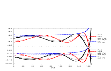
Figure 1: The $x$ and $y$ components and magnitude of the individual horizon momentum computed for the unequal mass black-hole binary with mass ratio $q=3/8$ until merger at $t\sim 164M$. Here $P$ denotes the quasi-local momentum and $\vec{V}=d\vec{y}/dt$.

III.2 Recoil momentum

In this section we study the recoil velocity of an already merged black-hole binary that acquires linear momentum as a reaction to the asymmetric radiation of gravitational waves during the inspiral and merger phases. We apply formula (3) to a single, slightly distorted, black hole and we attempt to compute speeds of the order $v/c\sim 0.0001$, which is three orders of magnitude smaller than the speeds in the orbital case.

We evolve two equal-mass black holes with opposite spins (pointing perpendicular to the line joining the holes), starting from rest, at an intermediate separation. The initial data parameters are summarized in Table 2. For this configuration the recoil momentum, as determined by an extrapolation of $\psi_{4}$ to $r=\infty$, is $P_{y}/M=(20.4\pm 0.5){\rm km\ s^{-1}}$ ($P_{x}=P_{z}=0$). We evolved these data using 9 levels of refinement with coarsest resolution $h=8M$ and finest resolution $h=M/32$, as well higher resolutions runs with finest resolutions of $M/48$ and $M/64$ (with a corresponding increase in gridpoints on all levels). Here we explore the dependence of the measured kick both on resolution and the $\eta$ parameter in Eq. (6). (Note that Eq. (5) approximates maximal slicing, i.e. $K\to 0$, at late times.)

Table 2: Initial data parameters for the equal mass opposite spinning black holes. The punctures are located along the $x$-axis starting from rest. Spins are denoted by $S_{i}$, puncture mass parameters by $m_{i}^{p}$, and horizon mass by $m_{i}^{H}$.

$x_{1}/M$	-3.5000	$m_{1}^{p}/M$	0.427644
$x_{2}/M$	+3.5000	$m_{2}^{p}/M$	0.427644
$S_{1}^{z}/M^{2}$	+0.15	$m_{1}^{H}/M$	0.517407
$S_{2}^{z}/M^{2}$	-0.15	$m_{2}^{H}/M$	0.517407
$P/M$	0.0000	$M_{\rm ADM}/M$	0.999998
$L^{z}/M^{2}$	0.0000	$J/M^{2}$	0.0000

The left panel of Fig. 2 shows the quasi-local recoil momentum versus time for $\eta=1$ and the three resolutions. Note the rapid convergence of the asymptotic value of the momentum versus resolution. The measured convergence rate is greater than 5, but even at a central resolution of $M/48$ the error in the recoil is within $3{\rm km\ s^{-1}}$. An extrapolation to infinite resolution gives $P_{y}/M=(21.5\pm 0.5){\rm km\ s^{-1}}$. The small disagreement between the quasi-local recoil and recoil calculated from $\psi_{4}$ is due to the use of a non-vanishing $\eta$. The right panel of Fig. 2 shows the dependence of the quasi-local momentum on the gauge via variations in $\eta$. Note that while $\eta$ has essentially no effect on the recoil calculated from $\psi_{4}$, the distortion in the gauge caused by large $\eta$ has a significant affect on the quasi-local momentum for $\eta>2$. In particular, for large $\eta$, the quasi-local momentum displays a slow secular decay towards a final asymptotic value, with both an increasing amplitude and decreasing decay rate, as $\eta$ is increased.

Note that the quasi-local formula provides an accurate measurement of the recoil at $t\sim 80M$, while a measurement based on $\psi_{4}$ requires evolutions of at least $150M$ for observers at $40M$.

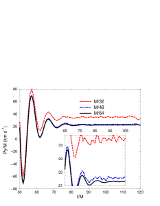
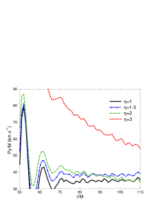
Figure 2: The remnant recoil velocity for the head-on test as determined by the isolated horizon formula. The panel on the left shows $P_{y}$ versus resolution for $\eta=1$. Note the rapid convergence of the asymptotic plateau. The panel on the right shows $P_{y}$ versus $\eta$ for $h=M/32$. The expected value of the recoil is $P_{y}/M=(20.4\pm 0.5){\rm km\ s^{-1}}$.

Figure 3 shows the quasi-local recoil momentum calculation for the orbiting binary configuration as a function of time and resolution. The expected recoil velocity in this case is $V=175{\rm km\ s^{-1}}$.

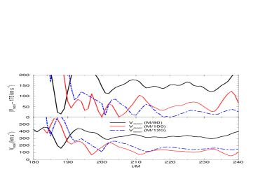
Figure 3: The recoil velocity of the remnant (bottom) and error (top) for the orbiting binary versus resolution for $\eta=2$.

IV Conclusion

There is currently no other fully relativistic method to compute the linear momentum of black holes in a binary. Knowledge of the linear momentum of each hole provides an important diagnostic in comparing fully-nonlinear results with post-Newtonian predictions of the trajectory and waveform (for instance as an alternative measure of the instantaneous angular velocity of the binary system).

The quasi-local approach we propose represents not only an alternative measure of the linear momentum, but also provides an accurate measurement of the recoil much sooner than can be obtained from the waveform.

In future work we will study a more coordinate independent and robust derivation of isolated horizon inspired formulae to evaluate the linear momentum of black holes. This can be achieved by an improved evaluation of the $\xi^{a}$ in addition to extrapolation to the $\eta\to 0$ and $h\to 0$ limits, and making greater use of the horizon geometry than was done here.