Large Deviation Principle for Self-Intersection Local Times for Random Walk in ${\mathbb{Z}}^{d}$ with $d\geq 5$.

Abstract

We obtain a large deviation principle for the self-intersection local times for a symmetric random walk in dimension $d\geq 5$. As an application, we obtain moderate deviations for random walk in random sceneries in Region II of [3].

Keywords and phrases: self-intersection local times, random walk, random scenery.

AMS 2000 subject classification numbers: 60K35, 82C22, 60J25.

Running head: LDP for self-intersections in $d\geq 5$.

1 Introduction.

We consider an aperiodic symmetric random walk on the lattice ${\mathbb{Z}}^{d}$, with $d\geq 5$. More precisely, if $S_{n}$ is the position of the walk at time $n\in{\mathbb{N}}$, then $S_{n+1}$ chooses uniformly at random a site of $\left\{{z\in{\mathbb{Z}}^{d}:|z-S_{n}|\leq 1}\right\}$, where for $z=(z_{1},\dots,z_{d})\in{\mathbb{Z}}^{d}$, the $l^{1}$-norm is $|z|:=|z_{1}|+\dots+|z_{d}|$. When $S_{0}=x$, we denote the law of this walk by $P_{x}$, and its expectation by $E_{x}$.

We are concerned with estimating the number of trajectories of length $n$ with many self-intersections, in the large $n$-regime. The self-intersection local times process reads as follows

$$\text{for }n\in{\mathbb{N}},\qquad B_{n}=\sum_{0\leq i<j<n}\hbox{1\hskip-3.0ptI}\{S_{i}=S_{j}\}.$$ (1.1)

The study of self-intersection local times has a long history in probability theory, as well as in statistical physics. Indeed, a caricature of a polymer would be a random walk self-interacting through short-range forces; a simple model arises as we penalize the simple random walk law with $\exp(\beta B_{n})$, where $\beta<0$ corresponds to a weakly self-avoiding walk, and $\beta>0$ corresponds to a self-attracting walk. The question is whether there is a transition from collapsed paths to diffusive paths, as we change the parameter $\beta$. We refer to Bolthausen’s Saint-Flour notes [5] for references and a discussion of these models.

It is useful to represent $B_{n}$ in terms of local times $\left\{{l_{n}(x),x\in{\mathbb{Z}}^{d}}\right\}$, that is the collection of number of visits of $x$ up to time $n$, as $x$ spans ${\mathbb{Z}}^{d}$. We set, for $k<n$,

$$l_{[k,n[}(x)=\hbox{1\hskip-3.0ptI}\{S_{k}=x\}+\dots+\hbox{1\hskip-3.0ptI}\{S_{n-1}=x\},l_{n}=l_{[0,n[},\quad\text{and}\quad||l_{n}||_{2}^{2}=\sum_{z\in{\mathbb{Z}}^{d}}l^{2}_{n}(z).$$ (1.2)

It is immediate that $||l_{n}||_{2}^{2}=2B_{n}+n$. Henceforth, we always consider $||l_{n}||_{2}^{2}$ rather than $B_{n}$. It turns out useful to think of the self-intersection local times as the square of the $l^{2}$-norm of an additive and positive process (see Section 7.3). Besides, we will deal with other $q$-norm of $l_{n}$ (see Proposition 1.4), for which there is no counterpart in terms of multiple self-intersections.

In dimensions $d\geq 3$, a random walk spends, on the average, a time of the order of one on most visited sites, whose number, up to time $n$, is of order $n$. More precisely, a result of [6] states

$$\frac{1}{n}||l_{n}||_{2}^{2}\stackrel{{\scriptstyle L^{2}}}{{\longrightarrow}}\gamma_{d}=2G_{d}(0)-1,\quad\text{with}\quad\forall z\in{\mathbb{Z}}^{d},\ G_{d}(z)=\sum_{n\geq 0}P_{0}(S_{n}=z).$$ (1.3)

The next question concerns estimating the probabilities of large deviations from the mean: that is $P_{0}(||l_{n}||_{2}^{2}-E_{0}[||l_{n}||_{2}^{2}]\geq n\xi)$ with $\xi>0$. In dimension $d\geq 5$, the speed of the large deviations is $\sqrt{n}$, and we know from [3] that a finite (random) set of sites, say ${\cal{D}}_{n}$, visited of the order of $\sqrt{n}$ makes a dominant contribution to produce the excess self-intersection.

However, in dimension 3, the correct speed for our large deviations is $n^{1/3}$ (see [1]), and the excess self-intersection is made up by sites visited less than some power of $\log(n)$. It is expected that the walk spends most of its time-period $[0,n]$ on a ball of radius of order $n^{1/3}$. Thus, in this box, sites are visited a time of order unity.

The situation is still different in dimension 2. First, $E_{0}[B_{n}]$ is of order $n\log(n)$, and a result of Le Gall [14] states that $\frac{1}{n}(B_{n}-E_{0}[B_{n}])$ converges in law to a non-gaussian random variable. The large (and moderate) deviations asymptotics obtained recently by Bass, Chen & Rosen in [4], reads as follows. There is some positive constant $C_{BCR}$, such that for any sequence $\left\{{b_{n},n\in{\mathbb{N}}}\right\}$ going to infinity with $\lim_{n\to\infty}\frac{b_{n}}{n}=0$, we have

$$\lim_{n\to\infty}\frac{1}{b_{n}}\log\left({P\left({B_{n}-E_{0}[B_{n}]\geq b_{n}n}\right)}\right)=-C_{BCR}.$$ (1.4)

For a LDP in the case of $d=1$, we refer to Chen and Li [7] (see also Mansmann [15] for the case of a Brownian motion instead of a random walk). In both $d=2$ and $d=1$, the result is obtained by showing that the local times of the random walk is close to its smoothened conterpart.

Finally, we recall a related result of Chen and Mörters [8] concerning mutual intersection local times of two independent random walks in infinite time horizon when $d\geq 5$. Let $l_{\infty}(z)=\lim_{n\to\infty}l_{n}(z)$, and denote by $\tilde{l}_{\infty}$ an independent copy of $l_{\infty}$. All symbols related to the second walk differ with a tilda. We denote the average over both walks by ${\mathbb{E}}$, and the product law is denoted ${\mathbb{P}}$. The intersection local times of two random walks, in an infinite time horizon, is

$$\left<{l_{\infty},\tilde{l}_{\infty}}\right>=\sum_{z\in{\mathbb{Z}}^{d}}l_{\infty}(z)\tilde{l}_{\infty}(z),\quad\text{and}\quad{\mathbb{E}}\left[{\left<{l_{\infty},\tilde{l}_{\infty}}\right>}\right]=\sum_{z\in{\mathbb{Z}}^{d}}G_{d}(z)^{2}<\infty,$$

where Green’s function, $G_{d}$, is square summable in dimension 5 or more. Chen and Mörters in [8] have obtained sharp asymptotics for $\{\langle l_{\infty},\tilde{l}_{\infty}\rangle\geq t\}$ for $t$ large, in dimension 5 or more, by an elegant asymptotic estimation of the moments, improving on the pioneering work of Khanin, Mazel, Shlosman and Sinai in [11]. Their method provides a variational formula for the rate functional, and their proof produces (and relies on) a finite volume version. Namely, for any finite subset $\Lambda\subset{\mathbb{Z}}^{d}$,

$$\lim_{t\to\infty}\frac{1}{\sqrt{t}}\log{\mathbb{P}}\left({\left<{\hbox{1\hskip-3.0ptI}_{\Lambda}l_{\infty},\tilde{l}_{\infty}}\right>\geq t}\right)=-2{\mathcal{I}}_{CM}(\Lambda),\quad\text{and}\quad\lim_{\Lambda\nearrow{\mathbb{Z}}^{d}}{\mathcal{I}}_{CM}(\Lambda)={\mathcal{I}}_{CM},$$ (1.5)

with

$${\mathcal{I}}_{CM}=\inf\left\{{||h||_{2}:\ h\geq 0,\ ||h||_{2}<\infty,\text{and}\ ||U_{h}||\geq 1}\right\},$$

where

$$U_{h}(f)(x)=\sqrt{e^{h(x)}-1}\sum_{y\in{\mathbb{Z}}^{d}}\left({G_{d}(x-y)-\delta_{x}(y)}\right)(f(y)\sqrt{e^{h(y)}-1}),$$ (1.6)

and $\delta_{x}$ is Kronecker’s delta function at $x$.

In this paper, we consider self-intersection local-times, and we establish a Large Deviations Principle in $d\geq 5$.

Theorem 1.1

We assume $d\geq 5$. There is a constant ${\mathcal{I}}(2)>0$, such that for $\xi>0$

$$\lim_{n\to\infty}\frac{1}{\sqrt{n}}\log P_{0}\left({||l_{n}||_{2}^{2}-E\left[{||l_{n}||_{2}^{2}}\right]\geq n\xi}\right)=-{\mathcal{I}}(2)\sqrt{\xi}.$$ (1.7)

Moreover,

$${\mathcal{I}}(2)={\mathcal{I}}_{CM}.$$ (1.8)

Remark 1.2

The reason for dividing Theorem 1.1 into two statements (1.7) and (1.8) is that our proof has two steps: (i) The proof of the existence of the limit in (1.7), which relies eventually on a subadditive argument, in spite of an odd scaling; (ii) An identification with the constant of Chen and Mörters.

Also, we establish later the existence of a limit for other $q$-norms of the local-times (see Proposition 1.4), for which we have no variational formulas.

The identification (1.8) relies on the fact that both the excess self-intersection local times and large intersection local times are essentially realized on a finite region. This is explained heuristically in Remark 1 of [8], and we provide the following mathematical statement of this latter phenomenon.

Proposition 1.3

Assume dimension is 5 or more.

$$\limsup_{\epsilon\to 0}\limsup_{t\to\infty}\frac{1}{\sqrt{t}}\log{\mathbb{P}}\left({\sum_{z\in{\mathbb{Z}}^{d}}\hbox{1\hskip-3.0ptI}_{\{\min(l_{\infty}(z),\tilde{l}_{\infty}(z))<\epsilon\sqrt{t}\}}l_{\infty}(z)\tilde{l}_{\infty}(z)>t}\right)=-\infty.$$ (1.9)

Finally, we present applications of our results to Random Walk in Random Sceneries (RWRS). We first describe RWRS. We consider a field $\{\eta(x),x\in{\mathbb{Z}}^{d}\}$ independent of the random walk $\{S_{k},k\in{\mathbb{N}}\}$, and made up of symmetric unimodal i.i.d.  with law denoted by ${\mathbb{Q}}$ and tail decay characterized by an exponent $\alpha>1$ and a constant $c_{\alpha}$ with

$$\lim_{t\to\infty}\frac{\log{\mathbb{Q}}\left({\eta(0)>t}\right)}{t^{\alpha}}=-c_{\alpha}.$$ (1.10)

The RWRS is the process

$$\left<{\eta,l_{n}}\right>:=\sum_{z\in{\mathbb{Z}}^{d}}\eta(z)l_{n}(z)=\eta(S_{0})+\dots+\eta(S_{n-1}).$$

We refer to [3] for references for RWRS, and for a diagram of the speed of moderate deviations $\left\{{\left<{\eta,l_{n}}\right>>\xi n^{\beta}}\right\}$ with $\xi>0$, in terms of $\alpha>1$ and $\beta>\frac{1}{2}$. In this paper, we concentrate on what has been called in [3] Region II:

$$1<\alpha<\frac{d}{2},\quad\text{and}\quad 1-\frac{1}{\alpha+2}<\beta<1+\frac{1}{\alpha}.$$ (1.11)

In region II, the random walk is expected to visit often a few sites, and it is therefore natural that our LDP allows for better asymptotics in this regime. We set

$$\zeta=\beta\frac{\alpha}{\alpha+1}(<1),\qquad\frac{1}{\alpha^{*}}=1-\frac{1}{\alpha},\quad\text{and for $\chi>0$}\quad\bar{\cal{D}}_{n}(\xi):=\left\{{z:\ l_{n}(z)\geq\xi}\right\}.$$ (1.12)

In bounding from above the probability of $\left\{{\left<{\eta,l_{n}}\right>\geq\xi\ n^{\beta}}\right\}$, we take exponential moments of $\left<{\eta,l_{n}}\right>$, and first integrate with respect to the $\eta$-variables. Thus, the behavior of the log-Laplace transform of $\eta$, say $\Gamma(x)=\log E\left[{\exp(x\eta(0))}\right]$, either at zero or at infinity, plays a key rôle. This, in turn, explains why we need a LDP for other powers of the local times. For $q\geq 1$, the $q$-norm of function $\varphi:{\mathbb{Z}}^{d}\to{\mathbb{R}}$ is

$$||\varphi||_{q}^{q}:=\sum_{z\in{\mathbb{Z}}^{d}}|\varphi(z)|^{q}.$$

Before dealing with $\left\{{\left<{\eta,l_{n}}\right>>\xi n^{\beta}}\right\}$, we give estimates for the ${\alpha^{*}}$-norm of the local-times, for $\alpha^{*}>\frac{d}{d-2}$.

Proposition 1.4

Choose $\zeta$ as in (1.12) with $\alpha,\beta$ in Region II. Choose $\chi$ such that $\zeta>\chi\geq\frac{\zeta}{d/2}$, and any $\xi>0$. There is a positive constant ${\mathcal{I}}(\alpha^{*})$ such that

$$\lim_{n\to\infty}\frac{1}{n^{\zeta}}\log\left({P\left({||\hbox{1\hskip-3.0ptI}_{\bar{\cal{D}}_{n}(n^{\chi})}l_{n}||_{\alpha^{*}}\geq\xi n^{\zeta}}\right)}\right)=-\xi\ {\mathcal{I}}(\alpha^{*}).$$ (1.13)

Our moderate deviations estimates for RWRS is as follows.

Theorem 1.5

Assume $\alpha,\beta$ are in Region II given in (1.11). With $\zeta$ given in (1.12), and any $\xi>0$

$$\lim_{n\to\infty}\frac{1}{n^{\zeta}}\log\left({P\left({\left<{\eta,l_{n}}\right>\geq\xi n^{\beta}}\right)}\right)=-c_{\alpha}(\alpha+1)\left({\frac{{\mathcal{I}}(\alpha^{*})}{\alpha}}\right)^{\frac{\alpha}{\alpha+1}}\quad\xi^{\frac{\alpha}{\alpha+1}}.$$ (1.14)

We now wish to outline schematically the main ideas and limitations in our approach. This serves also to describe the organisation of the paper. First, we use a shorthand notation for the centered self-intersection local times process,

$$\overline{||l_{n}||_{2}^{2}}=||l_{n}||_{2}^{2}-E_{0}\left[{||l_{n}||_{2}^{2}}\right].$$ (1.15)

Theorem 1.1 relies on the following intermediary result interesting on its own.

Proposition 1.6

Assume $d\geq 5$. There is $\beta>0$, such that for any $\epsilon>0$, there is $\alpha_{\epsilon}>0$, and $\Lambda_{\epsilon}$ a finite subset of ${\mathbb{Z}}^{d}$, such that for any $\alpha>\alpha_{\epsilon}$, for any $\Lambda\supset\Lambda_{\epsilon}$ finite, and $n$ large enough

$$\begin{split}\frac{1}{2}P_{0}\big{(}&||\hbox{1\hskip-3.0ptI}_{\Lambda}l_{\lfloor\alpha\sqrt{n}\rfloor}||_{2}^{2}\geq n\xi(1+\epsilon),\ S_{\lfloor\alpha\sqrt{n}\rfloor}=0\big{)}\\ &\leq P_{0}(\overline{||l_{n}||_{2}^{2}}\geq n\xi)\leq e^{\beta\epsilon\sqrt{n}}P_{0}\left({||\hbox{1\hskip-3.0ptI}_{\Lambda}l_{\lfloor\alpha\sqrt{n}\rfloor}||_{2}^{2}\geq n\xi(1-\epsilon),\ S_{\lfloor\alpha\sqrt{n}\rfloor}=0}\right).\end{split}$$ (1.16)

We use $\lfloor x\rfloor$ for the integer part of $x$.

The upper bound for $P_{0}(\overline{||l_{n}||_{2}^{2}}\geq n\xi)$ in (1.16) is the main technical result of the paper.

From our previous work in [3], we know that the main contribution to the excess self-intersection comes from level set ${\cal{D}}_{n}=\{x:l_{n}(x)\sim{\sqrt{n}}\}$. This is the place where $d\geq 5$ is crucial. Indeed, this latter fact is false in dimension 3 as shown in [1], and unknown in $d=4$. In Section 2, we recall and refine the results of [3]. We establish that ${\cal{D}}_{n}$ is a finite set. More precisely, for any $\epsilon>0$ and $L$ large enough, there is a constant $C_{\epsilon}$ such that for $n$ large enough

$$P\left({\overline{||l_{n}||_{2}^{2}}\geq n\xi}\right)\leq C_{\epsilon}\ P\left({||\hbox{1\hskip-3.0ptI}_{{\cal{D}}_{n}}l_{n}||_{2}^{2}\geq n\ \xi(1-\epsilon),\ |{\cal{D}}_{n}|<L}\right).$$ (1.17)

Then, our main objective is to show that the time spent on ${\cal{D}}_{n}$ is of order $\sqrt{n}$. However, this is only possible if some control on the diameter of ${\cal{D}}_{n}$ is first established. This is the main difficulty. Note that ${\cal{D}}_{n}$ is visited by the random walk within the time-period $[0,n[$, and from (1.17), a crude uniform estimate yields

$$P\left({\overline{||l_{n}||_{2}^{2}}\geq n\xi}\right)\leq C_{\epsilon}(2n)^{dL}\sup_{\Lambda\in]-n,n[^{d},|\Lambda|\leq L}\!\!\!P\left({||\hbox{1\hskip-3.0ptI}_{\Lambda}l_{n}||_{2}^{2}\geq n\ \xi(1-\epsilon)}\right).$$ (1.18)

Now, we can replace the time period $[0,n[$, in the right hand side of (1.18), by an infinite interval $[0,\infty)$ since the local time increases with time. Consider $\Lambda_{n}\subset]-n,n[^{d}$ which realizes the supremum in (1.18). Next, we construct two maps: a local map ${\cal{T}}$ in Section 3.2, and a global map $f$ in Section 5. A finite number of iterates of ${\cal{T}}$ (at most $L$), say ${\cal{T}}^{L}$, transforms $\Lambda_{n}$ into a subset of finite diameter. On the other hand, $f$ maps $\{{\cal{D}}_{n}=\Lambda_{n}\}$ into $\{{\cal{D}}_{n}={\cal{T}}(\Lambda_{n})\}$, allowing us to compare the probabilities of these two events. Thus, the heart of our argument has two ingredients.

• A marriage theorem which is recalled in Section 5.1. It is then used to perform global surgery on the circuits.

• Classical potential estimates of Sections 4.2 and 4.3. This is the place where the random walk’s features enter the play. Our estimates relies on basic estimates (Green’s function asymptotics, Harnack’s inequalities and heat kernel asymptotics), which are known to hold for general symmetric random walks (see [13]). Though we have considered the simplest aperiodic symmetric random walk, all our results hold when the basic potential estimates hold.

We then iterate $f$ a finite number of time to reach $\{{\cal{D}}_{n}={\cal{T}}^{L}(\Lambda_{n})\}$. To control the cost of this transformation, it is crucial that only a finite number of iterations of $f$ is needed. The construction of ${\cal{T}}$ and $f$ requires as well many preliminary steps.

1. Section 3 deals with clusters. In Section 3, we introduce a partition of $\Lambda_{n}$ into a collection of nearby points, called clusters. In Section 3.2, we define a map ${\cal{T}}$ acting on clusters, by translating one cluster at a time.

2. Section 4 deals with circuits. In Section 4.1, we decompose a trajectory in $\{{\cal{D}}_{n}=\Lambda_{n}\}$ into all possible circuits. We introduce the notions of trip and loop.

We show in Proposition 6.1, that for trajectories in $\{{\cal{D}}_{n}={\cal{T}}^{L}(\Lambda_{n})\}$, no time is wasted on lengthy excursions, and the total time needed to visit ${\cal{D}}_{n}$ is less than $\alpha{\sqrt{n}}$, for some large $\alpha$. This steps also relies on assuming $d\geq 5$. Indeed, we have been using that conditionned on returning to the origin, the expected return time is finite in dimension 5 or more. This concludes the outline of the proof of the upper bound in Proposition 1.6. The lower bound is easy, and is done in Section 7.2.

Assuming Proposition 1.6, we are in a situation where a certain $l^{2}$-norm of an additive process is larger than $\sqrt{n\xi}$ over a time-period of $\alpha{\sqrt{n}}$. Section 7.1 presents a subadditive argument yielding the existence of a limit (1.7). We identify the limit in Section 8.3. We prove Proposition 1.3 in Section 8. Finally, the proof of Theorem 1.5 is given in Section 9.

We conclude by mentionning two outstanding problems out of our reach.

• Establish a Large Deviations Principle in $d=3$, showing that the walk spends most of its time during time-period $[0,n[$, in a ball of radius about $n^{1/3}$.

• In dimension 4, find which level set of the local times gives a dominant contribution to making the self-intersection large.

2 Preliminaries on Level Sets.

In this section, we recall and refine the analysis of [3]. The approach of [2, 3] focuses on the contribution of each level set of the local times to the event $\{||l_{n}||_{2}^{2}-E[||l_{n}||_{2}^{2}]>n\xi\}$. This section is essentially a corollary of [3].

We first recall Proposition 1.6 of [3]. For $\epsilon_{0}>0$, set

$${\mathcal{R}}_{n}=\left\{{x\in{\mathbb{Z}}^{d}:n^{1/2-\epsilon_{0}}\leq l_{n}(x)\leq n^{1/2+\epsilon_{0}}}\right\}.$$

Then, for any $\epsilon>0$

$$\lim_{n\rightarrow\infty}\frac{1}{\sqrt{n}}\log P\left({||\hbox{1\hskip-3.0ptI}_{{\mathcal{R}}_{n}^{c}}l_{n}||_{2}^{2}-E_{0}\left[{||l_{n}||_{2}^{2}}\right]\geq n\epsilon\xi}\right)=-\infty\,.$$ (2.1)

Thus, we have for any $0<\epsilon<1$, and $\xi>0$

$$P\left({\overline{||l_{n}||_{2}^{2}}\geq n\xi}\right)\leq P\left({||\hbox{1\hskip-3.0ptI}_{{\mathcal{R}}_{n}^{c}}l_{n}||_{2}^{2}-E_{0}\left[{||l_{n}||_{2}^{2}}\right]\geq n\epsilon\xi}\right)+P\left({||\hbox{1\hskip-3.0ptI}_{{\mathcal{R}}_{n}}l_{n}||_{2}^{2}\geq n\xi(1-\epsilon)}\right).$$ (2.2)

We only need to focus on the second term of the right hand side of (2.2), and for simplicity here, we use $\xi>0$ instead of $\xi(1-\epsilon)$. First, we show in Lemma 2.1 that when asking $\{||l_{n}||_{2}^{2}\geq E[||l_{n}||_{2}^{2}]+n\xi\}$ with $\xi>0$, we can assume $\{||l_{n}||_{2}^{2}\leq An\}$ for some large $A$. Then, in Lemma 2.2, we show that the only sites which matter are those whose local times is within $[\frac{\sqrt{n}}{A},A\sqrt{n}]$ for some large constant $A$.

Lemma 2.1

For $A$ positive, there are constants $C,\kappa>0$ such that

$$P\left({\overline{||l_{n}||_{2}^{2}}\geq nA}\right)\leq C\exp\left({-\kappa\sqrt{An}}\right).$$ (2.3)

Proof.  We rely on Proposition 1.6 of [3], and the proof of Lemma 3.1 of [3] (with $p=2$ and $\gamma=1$), for the same subdivision $\left\{{b_{i},i=1,\dots,M}\right\}$ of $[1/2-\epsilon,1/2]$, and the same $\left\{{y_{i}}\right\}$ such that $\sum y_{i}\leq 1$, but the level sets are here of the form

$${\cal{D}}_{i}=\left\{{x\in{\mathbb{Z}}^{d}:\ A^{\frac{1}{2}}n^{b_{i}}\leq l_{n}(x)<A^{\frac{1}{2}}n^{b_{i+1}}}\right\}.$$ (2.4)

Using Lemma 2.2 of [3], we obtain the second line of (2.5),

$$P\left({\sum_{\cup{\cal{D}}_{i}}l_{n}^{2}(x)\geq nA}\right) \leq \sum_{i=1}^{M-1}P\left({|{\cal{D}}_{i}|(A^{\frac{1}{2}}n^{b_{i+1}})^{2}\geq ny_{i}A}\right)=\sum_{i=1}^{M-1}P\left({|{\cal{D}}_{i}|\geq y_{i}n^{1-2b_{i+1}}}\right)$$ (2.5)

$$\leq \sum_{i=1}^{M-1}(n^{d})^{n^{1-2b_{i+1}}y_{i}}\exp\left({-\kappa_{d}A^{\frac{1}{2}}n^{b_{i}+(1-\frac{2}{d})(1-2b_{i+1})}y_{i}^{1-\frac{2}{d}}}\right)$$ (2.5)

$$\leq \sup_{i\leq M}\left\{{{\cal{C}}_{i}(n)\exp\left({-\kappa_{d}A^{\frac{1}{2}}n^{b_{i}+(1-\frac{2}{d})(1-2b_{i+1})}y_{i}^{1-\frac{2}{d}}}\right)}\right\},$$ (2.5)

where ${\cal{C}}_{i}(n):=M(n^{d})^{n^{1-2b_{i+1}}y_{i}}$. The constant $\kappa_{d}$ is linked with estimating the probability of spending a given time in a given domain $\Lambda$ of prescribed volume; this latter inequality is derived in Lemma 1.2 of [2]. We first need ${\cal{C}}_{i}(n)$ to be negligible, which imposes

$$n^{1-2b_{i+1}}y_{i}\log(n^{d})\ll A^{\frac{1}{2}}n^{b_{i}+(1-\frac{2}{d})(1-2b_{i+1})}y_{i}^{1-\frac{2}{d}}$$ (2.6)

Inequality (2.6) is easily seen to hold when $b_{i}$ is larger than $1/2-\epsilon$, for $\epsilon$ small. Now, we need that for some $\kappa>0$

$$\kappa_{d}A^{\frac{1}{2}}n^{b_{i}+(1-\frac{2}{d})(1-2b_{i+1})}(y_{i})^{1-\frac{2}{d}}\geq 2\kappa A^{\frac{1}{2}}\sqrt{n}.$$ (2.7)

This holds with the choice of $y_{i}$ as in Lemma 3.1 of [3]. We use one $\kappa$ of (2.7) to match ${\cal{C}}_{i}(n)$ in (2.5), and we are left with a constant $C$ such that

$$P\left({\sum_{\cup{\cal{D}}_{i}}l_{n}^{2}(x)\geq nA}\right)\leq C\exp\left({-\kappa\sqrt{An}}\right)$$ (2.8)

 

For any positive reals $A$ and $\zeta$, an $k\in{\mathbb{N}}\cup\{\infty\}$, we define

$${\cal{D}}_{k}(A,\xi):=\left\{{x\in{\mathbb{Z}}^{d}:\frac{\xi}{A}\leq l_{k}(x)<A\xi}\right\}.$$ (2.9)

Lemma 2.2

Fix $\xi>0$. For any $M>0$, there is $A>0$ so that

$$\limsup_{n\to\infty}\frac{1}{\sqrt{n}}\log\left({P\left({\sum_{{\mathcal{R}}_{n}\backslash{\cal{D}}_{n}(A,\sqrt{n})}l_{n}^{2}(x)>n\xi}\right)}\right)\leq-M.$$ (2.10)

Also,

$$P\left({|{\cal{D}}_{n}(A,\sqrt{n})|\geq A^{3}}\right)\leq C\exp\left({-\kappa\sqrt{An}}\right).$$ (2.11)

Proof.  We consider an increasing sequence $\left\{{a_{i},i=1,\dots,N}\right\}$ to be chosen later, and form

$${\mathcal{B}}_{i}=\left\{{x:\ \frac{\sqrt{n}}{a_{i}}\leq l_{n}(x)<\frac{\sqrt{n}}{a_{i-1}}}\right\},$$ (2.12)

where $a_{0}$ will be chosen as a large constant, and $a_{N}\sim n^{\epsilon}$. In view of Lemma 2.1, it is enough to show that the probability of the event $\left\{{\sum_{{\mathcal{B}}_{i}}l_{n}^{2}(x)\geq n\xi}\right\}$ is negligible. First, from Lemma 2.1, we can restrict attention to $\left\{{An\geq\sum_{{\mathcal{B}}_{i}}l_{n}^{2}(x)\geq n\xi_{i}}\right\}$ for some large constant $A$ and with $\xi=\sum\xi_{i}$ a decomposition to be chosen later. When considering the sum over $x\in{\mathcal{B}}_{i}$, we obtain

$$\sum_{x\in{\mathcal{B}}_{i}}l_{n}^{2}(x)\leq nA\Longrightarrow|{\mathcal{B}}_{i}|\left({\frac{\sqrt{n}}{a_{i}}}\right)^{2}\leq An\Longrightarrow|{\mathcal{B}}_{i}|\leq a_{i}^{2}A.$$ (2.13)

Similarly, we obtain the lower bound $|{\mathcal{B}}_{i}|\geq\xi_{i}a_{i-1}^{2}$. If we call

$$H_{i}=\left\{{a_{i-1}^{2}\xi_{i}<|{\mathcal{B}}_{i}|\leq a_{i}^{2}A}\right\},$$ (2.14)

then by Lemma 2.1, if we set $l_{n}({\mathcal{B}}_{i})=\sum_{x\in{\mathcal{B}}_{i}}l_{n}(x)$

$$P\left({\sum_{x\in{\mathcal{B}}_{i}}l_{n}^{2}(x)>n\xi_{i}}\right) \leq P(\sum_{x\in{\mathcal{B}}_{i}}l_{n}^{2}(x)>nA))+P\left({H_{i}\cap\left\{{l_{n}({\mathcal{B}}_{i})\geq a_{i-1}\xi_{i}\sqrt{n}}\right\}}\right)$$ (2.15)

$$\leq Ce^{-\kappa\sqrt{An}}+(n^{d})^{a_{i}^{2}A}\exp\left({-\kappa_{d}\frac{a_{i-1}\xi_{i}\sqrt{n}}{(a_{i}^{2}A)^{2/d}}}\right).$$ (2.15)

Since we assume $a_{i}\leq n^{\epsilon}$, the term $(n^{d})^{a_{i}^{2}A}$ is innocuous. It remains to find, for any large constant $M$, two sequences $\left\{{a_{i},\xi_{i},i=1,\dots,N}\right\}$ such that

$$\kappa_{d}\frac{a_{i-1}\xi_{i}}{(a_{i}^{2}A)^{2/d}}=M,\quad\text{and}\quad\sum\xi_{i}=\xi.$$ (2.16)

Fix an arbitrary $\delta>0$ and set

$$a_{i}:=(1+\delta)^{i}a_{0},\quad\xi_{i}:=\frac{z(\delta)}{(1+\delta)^{\gamma i}}\xi,\quad\text{and}\quad\gamma=1-\frac{4}{d},$$ (2.17)

where $z(\delta)$ is a normalizing constant ensuring that $\sum\xi_{i}=\xi$. Using the values (2.17) in (2.16), we obtain

$$\frac{\kappa_{d}z(\delta)\xi}{(1+\delta)A^{2/d}}a_{0}^{1-4/d}=M.$$ (2.18)

Now, for any constant $M$, we can choose an $a_{0}$ large enough so that none of the level ${\mathcal{B}}_{i}$ contributes. Note also that $N=\min\left\{{n:a_{n}\geq n^{\epsilon}}\right\}$.

Finally, (2.11) follows from Lemma 2.1, once we note that

$$P\left({|{\cal{D}}_{n}(A,\sqrt{n})|\geq A^{3}}\right)\leq P\left({||\hbox{1\hskip-3.0ptI}_{{\cal{D}}_{n}(A,\sqrt{n})}l_{n}||_{2}^{2}\geq An}\right).$$

 

We will need estimates for other powers of the local times. We choose two parameters $(\alpha,\beta)$ satisfying (1.11), and we further define

$$\zeta=\beta\frac{\alpha}{\alpha+1},\qquad b=\frac{\beta}{\alpha+1},\qquad\frac{1}{\alpha^{*}}=1-\frac{1}{\alpha},\quad\text{and}\quad\bar{\cal{D}}_{n}(n^{b}):=\left\{{z:\ l_{n}(z)\geq n^{b}}\right\}.$$ (2.19)

When dealing with the $\alpha^{*}$-norm of $l_{n}$, we only focus on sites with large local times. Among those sites, we show that finitely many contribute to making the $\alpha^{*}$-norm of $l_{n}$ large. To appreciate the first estimate, similar in spirit and proof to Lemma 2.2, recall that $\zeta<1$, $\alpha^{*}>1$, and $||l_{n}||_{\alpha^{*}}\geq||l_{n}||_{1}=n$.

Lemma 2.3

Choose $\zeta,b$ as in (2.19) with $\alpha,\beta$ in Region II. For any $\xi>0$, there are constants $C,\kappa>0$ such that

$$P\left({||\hbox{1\hskip-3.0ptI}_{\bar{\cal{D}}_{n}(n^{b})}l_{n}||_{\alpha^{*}}\geq\xi n^{\zeta}}\right)\leq C\exp\left({-\kappa\xi n^{\zeta}}\right).$$ (2.20)

Moreover, for any $M>0$, there is $A>0$ such that

$$\limsup_{n\to\infty}\frac{1}{n^{\zeta}}\log P\left({||\hbox{1\hskip-3.0ptI}_{{\cal{D}}_{n}(A,n^{\zeta})^{c}\cap\bar{\cal{D}}_{n}(n^{b})}l_{n}||_{\alpha^{*}}>\xi n^{\zeta}}\right)\leq-M.$$ (2.21)

Finally, from (2.20), we have

$$P\left({|{\cal{D}}_{n}(A,n^{\zeta})|\geq A^{2}}\right)\leq P\left({||\hbox{1\hskip-3.0ptI}_{{\cal{D}}_{n}(A,n^{\zeta})}l_{n}||_{\alpha^{*}}\geq An^{\zeta}}\right)\leq C\exp\left({-\kappa An^{\zeta}}\right).$$ (2.22)

The proof is similar to that of Lemmas 2.1 and  2.2, and we omit the details. We point out that Lemma 3.1 of [3] has to be used with $p=\alpha^{*}$ and $\gamma=\alpha^{*}\zeta$. Also, Proposition 3.3 of [3] holds on $\bar{\cal{D}}_{n}(n^{b})$ since the condition $b\frac{d}{2}\geq\zeta$ is fulfilled in Region II.

3 Clusters’ Decomposition.

From Lemma 2.2, for any $\epsilon>0$, and $A$ large enough, we have $C_{\epsilon}>0$ such that for any $\xi>0$ and $n$ large enough

$$P\left({\overline{||l_{n}||_{2}^{2}}\geq n\xi(1+\epsilon)}\right)\leq C_{\epsilon}P\left({||\hbox{1\hskip-3.0ptI}_{{\cal{D}}_{n}(A,\sqrt{n})}l_{n}||_{2}^{2}\geq n\xi,\ |{\cal{D}}_{n}(A,\sqrt{n})|\leq A^{3}}\right).$$ (3.1)

Since ${\cal{D}}_{n}(A,\sqrt{n})\subset]-n,n[^{d}$, we bound the right hand side of (3.1) by a uniform bound

$$\begin{split}P\left({\overline{||l_{n}||_{2}^{2}}\geq n\xi(1+\epsilon)}\right)\leq&C_{\epsilon}(2n)^{dA^{3}}\sup_{\Lambda}P\left({||\hbox{1\hskip-3.0ptI}_{\Lambda}l_{n}||_{2}^{2}\geq n\xi,{\cal{D}}_{n}(A,\sqrt{n})=\Lambda}\right)\\ \leq&C_{\epsilon}(2n)^{dA^{3}}\sup_{\Lambda}P\left({||\hbox{1\hskip-3.0ptI}_{\Lambda}l_{\infty}||_{2}^{2}\geq n\xi,\Lambda\subset{\cal{D}}_{\infty}(A,\sqrt{n})}\right),\end{split}$$ (3.2)

where in the supremum over $\Lambda$ we assumed that $\Lambda\subset]-n,n[^{d},\ |\Lambda|\leq A^{3}$. Also, in ${\cal{D}}_{\infty}(A,\sqrt{n})$ (defined in (2.9)) we may adjust with a larger $A$ if necessary.

If we denote by $\Lambda_{n}$ the finite subset of ${\mathbb{Z}}^{d}$ which realizes the last supremum in (3.2), then our starting point, in this section, is the collection $\{\Lambda_{n},n\in{\mathbb{N}}\}$ of finite subsets of ${\mathbb{Z}}^{d}$.

3.1 Defining Clusters.

In this section, we partition an arbitrary finite subset of ${\mathbb{Z}}^{d}$, say $\Lambda$ into subsets of nearby sites, with the feature that these subsets are far apart. More precisely, this partitioning goes as follows.

Lemma 3.1

Fix $\Lambda$ finite subset of ${\mathbb{Z}}^{d}$, and $L$ an integer. There is a partition of $\Lambda$ whose elements are called $L$-clusters with the property that two distinct $L$-clusters ${\cal{C}}$ and $\tilde{\cal{C}}$ satisfy

$$\text{dist}({\cal{C}},\tilde{\cal{C}}):=\inf\left\{{|x-y|,\ x\in{\cal{C}},y\in\tilde{\cal{C}}}\right\}\geq 4\max\left({\text{diam}({\cal{C}}),\text{diam}(\tilde{\cal{C}}),L}\right).$$ (3.3)

Also, there is a positive constant $C(\Lambda)$ which depends on $|\Lambda|$, such that for any $L$-cluster ${\cal{C}}$

$$\text{diam}({\cal{C}})\leq C(\Lambda)\ L.$$ (3.4)

Remark 3.2

If we define an $L$-shell ${\cal{S}}_{L}({\cal{C}})$ around ${\cal{C}}$ by

$${\cal{S}}_{L}({\cal{C}})=\left\{{z\in{\mathbb{Z}}^{d}:\ \text{dist}(z,{\cal{C}})\leq\max(L,\text{diam}({\cal{C}}))}\right\},\quad\text{ then }\quad{\cal{S}}_{L}({\cal{C}})\cap\Lambda={\cal{C}}.$$ (3.5)

We deduce from (3.4), and (3.5), that for any ${\cal{C}}$ and any $x,y\in{\cal{C}}$, there is a finite sequence of points $x_{0}=x,\dots,x_{k}=y$ (not necessarely in $\Lambda$), such that for $i=1,\dots,k$

$$|x_{i}-x_{i-1}|\leq L,\quad\text{and}\quad B(x_{i},L)\subset{\cal{S}}({\cal{C}})\quad(\text{where }B(x_{i},L)=\left\{{z\in{\mathbb{Z}}^{d}:\ |x_{i}-z|\leq L}\right\}).$$ (3.6)

Proof.  We build clusters by a bootstrap algorithm. At level 0, we define a linking relation for $x,y\in\Lambda$: $x\overset{0}{\leftrightarrow}y$ if $|x-y|\leq 4L$, and an equivalent relation $x\overset{0}{\sim}y$ if there is a (finite) path $x=x_{1},x_{2},\dots,x_{k}=y\in\Lambda$ such that for $i=1,\dots,k-1$, $x_{i}\overset{0}{\leftrightarrow}x_{i+1}$. The cluster at level 0 are the equivalent classes of $\Lambda$. We denote by ${\cal{C}}^{(0)}(x)$ the class which contains $x$, and by $|{\cal{C}}^{(0)}|$ the number of clusters at level 0 which is bounded by $|\Lambda|$. It is important to note that the diameter of a cluster is bounded independently of $n$. Indeed, it is easy to see, by induction on $|\Lambda|$, that for any $x\in\Lambda$, we have $\text{diam}({\cal{C}}^{(0)}(x))\leq 4L(|{\cal{C}}^{(0)}(x)|-1)$, so that

$$\text{diam}({\cal{C}}^{(0)}(x))\leq 4L|\Lambda|.$$ (3.7)

Then, we set

$$x\overset{1}{\leftrightarrow}y\quad\text{if}\quad|x-y|\leq 4\max\left({\text{diam}({\cal{C}}^{(0)}(x)),\text{diam}({\cal{C}}^{(0)}(y)),L}\right).$$ (3.8)

As before, relation $\overset{1}{\leftrightarrow}$ is associated with an equivalence relation $\overset{1}{\sim}$ which defines clusters ${\cal{C}}^{(1)}$. Note also that $x\overset{0}{\sim}y$ implies that $x\overset{1}{\sim}y$, and that for any $x\in\Lambda$,

$$\text{diam}({\cal{C}}^{(1)}(x))\leq 5|{\cal{C}}^{(0)}|\max\left\{{\text{diam}({\cal{C}}):\ {\cal{C}}\in{\cal{C}}^{(0)}}\right\}\leq 5|\Lambda|(4L|\Lambda|),$$ (3.9)

since we produce ${\cal{C}}^{(1)}$’s by multiple concatenations of pairs of ${\cal{C}}^{(0)}$-clusters at a distance of at most four times the maximum diameters of the clusters making up level 0, those latter clusters being less in number than $|\Lambda|$. In the worst scenario, there is one cluster at level 1 made up of all clusters of ${\cal{C}}^{(0)}$ at a distance of at most $4\max\left\{{\text{diam}({\cal{C}}):\ {\cal{C}}\in{\cal{C}}^{(0)}}\right\}$.

If the number of clusters at level 0 is the same as those of level 1, then the algorithm stops and we have two distinct clusters ${\cal{C}},\tilde{\cal{C}}\in{\cal{C}}^{(0)}$

$$\text{dist}({\cal{C}},\tilde{\cal{C}}):=\inf\left\{{|x-y|,\ x\in{\cal{C}},y\in\tilde{\cal{C}}}\right\}\geq 4\max\left({\text{diam}({\cal{C}}),\text{diam}(\tilde{\cal{C}}),L}\right).$$

Otherwise, the number of cluster at level 1 has decreased by at least one. Now, assume by way of induction, that we have reached level $k-1$. We define $\overset{k}{\leftrightarrow}$ as follows

$$x\overset{k}{\leftrightarrow}y\quad\text{if}\quad|x-y|\leq 4\max\left({\text{diam}({\cal{C}}^{(k-1)}(x)),\text{diam}({\cal{C}}^{(k-1)}(y)),L}\right).$$ (3.10)

Now, since $|\Lambda|$ is finite, the algorithm stops in a finite number of steps. The clusters we obtain eventually are called $L$-clusters. Note that two distinct $L$-clusters satisfy (3.3). Property (3.4) with $C(\Lambda)=(5|\Lambda|)^{|\Lambda|}$, follows by induction with the same argument used to prove (3.9).  

3.2 Transforming Clusters.

For a subset $\Lambda$ and an integer $L$, assume that we have a partition in terms of $L$-cluster as in Lemma 3.1. We define the following map on the partition of $\Lambda$.

Lemma 3.3

There is a map ${\cal{T}}$ on the $L$-clusters of $\Lambda$ such that ${\cal{T}}({\cal{C}})={\cal{C}}$, but for one cluster, say ${\cal{C}}_{1}$ where ${\cal{T}}({\cal{C}}_{1})$ is a translate of ${\cal{C}}_{1}$ such that, when the following minimun is taken over all $L$-clusters

$$0=\min\left\{{\text{dist}\left({{\cal{C}},{\cal{T}}({\cal{C}}_{1})}\right)-\left({\text{diam}({\cal{C}})+\text{diam}({\cal{T}}({\cal{C}}_{1})}\right)}\right\}.$$ (3.11)

Also, for any $L$-cluster ${\cal{C}}\not={\cal{C}}_{1}$, we have

$$\text{dist}({\cal{C}},{\cal{T}}({\cal{C}}_{1}))\leq 2\text{dist}({\cal{C}},{\cal{C}}_{1}).$$ (3.12)

We denote by ${\cal{T}}(\Lambda)=\cup\ {\cal{T}}({\cal{C}})$. Also, we can define ${\cal{T}}$ as a map on ${\mathbb{Z}}^{d}$: for a site $z\in{\cal{C}}_{1}$ ${\cal{T}}(z)$ denotes the translation of $z$, otherwise ${\cal{T}}(z)=z$. Finally, we can define the inverse of ${\cal{T}}$, which we denote ${\cal{T}}^{-1}$.

Remark 3.4

Note that ${\cal{T}}(\Lambda)$ has at least one $L$-cluster less than $\Lambda$ since (3.3) does not hold for $({\cal{C}}_{0},{\cal{T}}({\cal{C}}_{1}))$. Thus, if we apply to $L$-cluster partition of Lemma 3.1 to ${\cal{T}}(\Lambda)$, ${\cal{C}}_{0}$ and ${\cal{T}}({\cal{C}}_{1})$ would merge into one $L$-cluster, possibly triggering other merging.

Proof.  We start with two clusters which minimize the distance among clusters. Let ${\cal{C}}_{0}$ and ${\cal{C}}_{1}$ be such that

$$\text{dist}({\cal{C}}_{0},{\cal{C}}_{1})=\min\left\{{\text{dist}({\cal{C}},{\cal{C}}^{\prime}):\ {\cal{C}},{\cal{C}}^{\prime}\text{ distinct clusters}}\right\}.$$ (3.13)

Now, let $(x_{0},x_{1})\in{\cal{C}}_{0}\times{\cal{C}}_{1}$ such that $|x_{0}-x_{1}|=\text{dist}({\cal{C}}_{0},{\cal{C}}_{1})$, and note that by (3.3), $|x_{0}-x_{1}|\geq 2\left({\text{diam}({\cal{C}}_{0})+\text{diam}({\cal{C}}_{1})}\right)$. Assume that $\text{diam}({\cal{C}}_{0})\geq\text{diam}({\cal{C}}_{1})$. We translate sites of ${\cal{C}}_{1}$ by a vector whose coordinates are the integer parts of the following vector

$$u=(x_{0}-x_{1})\left({1-\frac{\text{diam}({\cal{C}}_{0})+\text{diam}({\cal{C}}_{1})}{|x_{0}-x_{1}|}}\right),$$ (3.14)

in such a way that the translated cluster, say ${\cal{T}}({\cal{C}}_{1})$, is at a distance $\text{diam}({\cal{C}}_{0})+\text{diam}({\cal{C}}_{1})$ of ${\cal{C}}_{0}$. We now see that ${\cal{T}}({\cal{C}}_{1})$ is far enough from other clusters. Let, as before, $z\in{\cal{C}}$, and note that

$$|z-\tilde{y}| \geq |z-x_{0}|-|x_{0}-\tilde{y}|\geq|z-x_{0}|-\left({|x_{0}-\tilde{x}_{1}|+|\tilde{x}_{1}-\tilde{y}|}\right)$$ (3.15)

$$\geq 4\max(\text{diam}({\cal{C}}),\text{diam}({\cal{C}}_{0}))-\left({\text{diam}({\cal{C}}_{0})+\text{diam}({\cal{C}}_{1})+\text{diam}({\cal{C}}_{1})}\right)$$ (3.15)

$$\geq \text{diam}({\cal{C}})+\text{diam}({\cal{C}}_{1})$$ (3.15)

Thus, for any cluster ${\cal{C}}$, we have

$$\text{dist}({\cal{C}},{\cal{T}}({\cal{C}}_{1}))\geq\text{diam}({\cal{C}})+\text{diam}({\cal{T}}({\cal{C}}_{1})).$$ (3.16)

Finally, we prove (3.12). Let $z$ belong to say ${\cal{C}}\not={\cal{C}}_{1}$, and let $\tilde{y}\in{\cal{T}}({\cal{C}}_{1})$ be the image of $y\in{\cal{C}}_{1}$ after translation by $u$. Then, using that $\text{dist}({\cal{C}}_{0},{\cal{C}}_{1})$ minimizes the distance among distinct clusters

$$|z-\tilde{y}| \leq |z-y|+|y-\tilde{y}|\leq|z-y|+\text{dist}({\cal{C}}_{0},{\cal{C}}_{1})$$ (3.17)

$$\leq |z-y|+\text{dist}({\cal{C}},{\cal{C}}_{1})\leq 2|z-y|.$$ (3.17)

 

4 On Circuits.

4.1 Definitions and Notations.

Let $\Lambda_{n}\subset{\mathbb{Z}}^{d}$ maximizes the supremum in the last term of (3.2). Assume we have partitioned $\Lambda_{n}$ into $L$-clusters, as done in Section 3.

We decompose the paths realizing $\{||1_{\Lambda_{n}}l_{\infty}||_{2}^{2}\geq n\xi\}$ with $\{\Lambda_{n}\subset{\cal{D}}_{\infty}(A,\sqrt{n})\}$ into the successive visits to $\Lambda_{n}^{\prime}=\Lambda_{n}\cup{\cal{T}}(\Lambda_{n})$. For ease of notations, we drop the subscript $n$ in $\Lambda$ though it is important to keep in mind that $\Lambda$ varies as we increase $n$.

We consider the collection of integer-valued vectors over $\Lambda^{\prime}$ which we think of as candidates for the local times over $\Lambda^{\prime}$. Thus

$$V(\Lambda^{\prime},n):=\left\{{{\bf k}\in{\mathbb{N}}^{\Lambda^{\prime}}:\ \inf_{x\in\Lambda}k(x)\geq\frac{\sqrt{n}}{A},\ \sup_{x\in\Lambda^{\prime}}k(x)\leq A{\sqrt{n}},\quad\sum_{x\in\Lambda}k^{2}(x)\geq n\xi}\right\}.$$ (4.1)

Also, for ${\bf k}\in V(\Lambda^{\prime},n)$, we set

$$|{\bf k}|=\sum_{x\in\Lambda^{\prime}}k(x),\quad\text{and note that}\quad|{\bf k}|\leq|\Lambda^{\prime}|A{\sqrt{n}}\leq 2A^{4}{\sqrt{n}}.$$ (4.2)

We need now more notations. For $U\subset{\mathbb{Z}}^{d}$, we call $T(U)$ the first hitting time of $U$, and we denote by $T:=T(\Lambda^{\prime})=\inf\left\{{n\geq 0:S_{n}\in\Lambda^{\prime}}\right\}$. We also use the notation $\tilde{T}(U)=\inf\left\{{n\geq 1:S_{n}\in U}\right\}$. For a trajectory in the event $\left\{{l_{\infty}(x)=k(x),\forall x\in\Lambda^{\prime}}\right\}$, we call $\left\{{T^{(i)},i\in{\mathbb{N}}}\right\}$ the successive times of visits of $\Lambda^{\prime}$: $T^{(1)}=\inf\left\{{n\geq 0:S_{n}\in\Lambda^{\prime}}\right\}$, and by induction for $i\leq|{\bf k}|$ when $\left\{{T^{(i-1)}<\infty}\right\}$

$$T^{(i)}=\inf\left\{{n>T^{(i-1)}:S_{n}\in\Lambda^{\prime}}\right\}.$$ (4.3)

The first observation is that the number of long trips cannot be too large.

Lemma 4.1

For any $\epsilon>0$, and $M>0$, there is $L>0$ such that for each ${\bf k}\in V(\Lambda^{\prime},n)$,

$$P\left({l_{\infty}|_{\Lambda^{\prime}}={\bf k},\ \big{|}\left\{{i\leq|{\bf k}|:\ |S_{T^{(i)}}-S_{T^{(i-1)}}\big{|}>{\sqrt{L}}}\right\}|\geq\epsilon{\sqrt{n}}}\right)\leq e^{-M{\sqrt{n}}}.$$ (4.4)

We know from [3] that the probability that $\{\overline{||l_{n}||_{2}^{2}}\geq n\xi\}$ is bounded from below by $\exp(-\bar{c}\sqrt{n})$ for some positive constant $\bar{c}$. We assume $M>2\bar{c}$ (and $L>L(M)$ given in Lemma 4.1), and the left hand side of (4.4) is negligible. The proof of this Lemma is postponed to the Appendix.

We consider now the collections of possible sequence of visited sites of $\Lambda^{\prime}$, and in view of Lemma 4.1, we consider at most $\epsilon{\sqrt{n}}$ consecutive sites at a distance larger than ${\sqrt{L}}$. First, for ${\bf k}\in V(\Lambda^{\prime},n)$, and each ${\bf z}\in{\cal{E}}({\bf k})$, and $x\in{\mathbb{Z}}^{d}$, we denote by $l_{{\bf z}}(x)$ the local times of ${\bf z}$ at $x$, that is the number of occurrences of $x$ in the string ${\bf z}$. Then,

$${\cal{E}}({\bf k})=\left\{{{\bf z}\in(\Lambda^{\prime})^{|{\bf k}|}:\ l_{{\bf z}}(x)=k(x),\forall x\in\Lambda^{\prime},\quad\sum_{i<|{\bf k}|}\hbox{1\hskip-3.0ptI}_{\left\{{|z(i+1)-z(i)|>{\sqrt{L}}}\right\}}<\epsilon{\sqrt{n}}}\right\}.$$ (4.5)

Definition 4.2

For ${\bf k}\in V(\Lambda^{\prime},n)$, a circuit is an element of ${\cal{E}}({\bf k})$. The random walk follows circuit ${\bf z}\in{\cal{E}}({\bf k})$, if it belongs to the event

$$\left\{{S_{T^{(i)}}=z(i),i=1,\dots,|{\bf k}|}\right\}\cap\left\{{T^{(|{\bf k}|+1)}=\infty}\right\}.$$ (4.6)

When we lift the second constrain in (4.6), we obtain when $L$ is large enough (with the convention $z(0)=0$)

$$P\left({||\hbox{1\hskip-3.0ptI}_{\Lambda}l_{\infty}||_{2}^{2}\geq n\xi,\ \Lambda\subset{\cal{D}}_{\infty}(A,\sqrt{n})}\right)\leq 2\sum_{{\bf k}\in V(\Lambda^{\prime},n)}\sum_{{\bf z}\in{\cal{E}}({\bf k})}\prod_{i=1}^{|{\bf k}|}P_{z(i-1)}\left({S_{T}=z(i)}\right).$$ (4.7)

We come now to the definitions of trips and loops.

Definition 4.3

Let ${\bf k}\in V(\Lambda^{\prime},n)$ and ${\bf z}\in{\cal{E}}({\bf k})$. A trip is a pair $(z(i),z(i+1))$, where $z(i)$ and $z(i+1)$ do not belong to the same cluster. A loop is a maximal substring of ${\bf z}$ belonging to the same cluster.

Remark 4.4

We think of a circuit as a succession of loops connected by trips. Recall that (3.3) tells us that two points of a trip are at a distance larger than $L$. Thus, trips are necessarely long journeys, whereas loops may contain many short journeys, typically of the order of $\sqrt{n}$. For ${\bf z}\in{\cal{E}}({\bf k})$, the number of trips is less than $\epsilon{\sqrt{n}}$, so is the number of loops, since a loop is followed by a trip.

We recall the notations of Section 3.2: $\Lambda=\{{\cal{C}}_{0},{\cal{C}}_{1},\dots,{\cal{C}}_{k}\}$ with $\text{dist}({\cal{C}}_{0},{\cal{C}}_{1})$ minimizing distance among the clusters. The map ${\cal{T}}$ translates only cluster ${\cal{C}}_{1}$.

We now fix ${\bf k}\in V(\Lambda^{\prime},n)$ and ${\bf z}\in{\cal{E}}({\bf k})$. We number the different points of entering and exiting from ${\cal{C}}_{1}$.

$$\tau_{1}=\inf\left\{{n>0:\ z(n)\in{\cal{C}}_{1}}\right\},\quad\text{and}\quad\sigma_{1}=\inf\left\{{n>\tau_{1}:\ z(n)\not\in{\cal{C}}_{1}}\right\},$$ (4.8)

and by induction, if we assume $\left\{{\tau_{2},\sigma_{2},\dots,\tau_{i},\sigma_{i}}\right\}$ defined with $\sigma_{i}<\infty$, then

$$\tau_{i+1}=\inf\left\{{n>\sigma_{i}:\ z(n)\in{\cal{C}}_{1}}\right\},\quad\text{and}\quad\sigma_{i+1}=\inf\left\{{n>\tau_{i+1}:\ z(n)\not\in{\cal{C}}_{1}}\right\}.$$ (4.9)

Definition 4.5

For a configuration ${\bf z}\in{\cal{E}}({\bf k})$, its $i$-th ${\cal{C}}_{1}$-loop is

$${\cal{L}}(i)=\left\{{z(\tau_{i}),z(\tau_{i}+1),\dots,z(\sigma_{i}-1)}\right\}.$$ (4.10)

We associate with ${\cal{L}}(i)$ the entering and exiting site from ${\cal{C}}_{1}$, $p(i)=\left\{{z(\tau_{i}),z(\sigma_{i}-1)}\right\}$, which we think of as the type of the ${\cal{C}}_{1}$-loop.

The construction is identical for ${\cal{T}}({\cal{C}}_{1})$ (usually with a tilda put on all symbols).

4.2 Encaging Loops.

We wish eventually to transform a piece of random walk associated with a ${\cal{C}}_{1}$-loop, into a piece of random walk associated with a ${\cal{T}}({\cal{C}}_{1})$-loop. We explain one obvious problem we face when acting with ${\cal{T}}$ on circuits. Consider a ${\cal{C}}_{1}$-loop in a circuit ${\bf z}$. Assume for simplicity, that it corresponds to the $i$-th ${\cal{C}}_{1}$-loop. In general,

$$\prod_{k=\tau_{i}}^{\sigma_{i}-2}P_{z(k)}\left({S_{T}=z(k+1)}\right)\quad\not=\quad\prod_{k=\tau_{i}}^{\sigma_{i}-2}P_{{\cal{T}}(z(k))}\left({S_{T}={\cal{T}}(z(k+1))}\right).$$ (4.11)

However, if while travelling from $z(k)$ to $z(k+1)$, the walk were forced to stay inside an $L$-shell of ${\cal{C}}_{1}$ during $[\tau_{i},\sigma_{i}[$, then under ${\cal{T}}$, we would have a walk travelling from ${\cal{T}}(z(k))$ to ${\cal{T}}(z(k+1))$, inside an $L$-shell of ${\cal{T}}({\cal{C}}_{1})$.

To give a precise meaning to our use of the expression encage, we recall that for any cluster ${\cal{C}}$, the $L$-shell around ${\cal{C}}$ is denoted

$${\cal{S}}({\cal{C}})=\left\{{z:\ \text{dist}(z,{\cal{C}})=\max(L,\text{diam}({\cal{C}}))}\right\}.$$

Now, for $x,y\in{\cal{C}}$, the random walk is encaged inside $S$ while flying from $x$ to $y$ if it does not exit ${\cal{S}}$ before touching $y$. The main result in this section is the following proposition.

Proposition 4.6

Fix a circuit ${\bf z}\in{\cal{E}}({\bf k})$ with ${\bf k}\in V(\Lambda,n)$. For any $\epsilon>0$, there is $L$ integer, and a constant $\beta>0$ independent of $\epsilon$, such that if ${\cal{C}}_{i}:={\cal{C}}(z(i))$, and

$$\begin{split}P^{L}_{z(i)}\left({S_{T}=z(i+1)}\right)=&\hbox{1\hskip-3.0ptI}_{\left\{{z(i+1)\in{\cal{C}}_{i}}\right\}}P_{z(i)}\left({S_{T}=z(i+1),T<T({\cal{S}}({\cal{C}}_{i}))}\right)\\ &\quad+\hbox{1\hskip-3.0ptI}_{\left\{{z(i+1)\not\in{\cal{C}}_{i}}\right\}}P_{z(i)}\left({S_{T}=z(i+1)}\right),\end{split}$$ (4.12)

then

$$\prod_{i=0}^{|{\bf k}|-1}P_{z(i)}\left({S_{T}=z(i+1)}\right)\leq e^{\beta\epsilon{\sqrt{n}}}\prod_{i=0}^{|{\bf k}|-1}P^{L}_{z(i)}\left({S_{T}=z(i+1)}\right).$$ (4.13)

Remark 4.7

Consider a ${\cal{C}}$-loop, say ${\cal{L}}$, and assume that for some integer $i$, ${\cal{L}}$ corresponds to the $i$-th ${\cal{C}}$-loop in circuit ${\bf z}$. We use the shorthand notation $\text{Weight}({\cal{L}})$ to denote the probability associated with ${\cal{L}}$

$$\text{Weight}({\cal{L}}):=\prod_{k=\tau_{i}}^{\sigma_{i}}P^{L}_{z(k-1)}\left({S_{T}=z(k)}\right).$$ (4.14)

Note that $\text{Weight}({\cal{L}})$ includes the probabilities of the entering and exiting trip. The point of encaging loop is the following identity

$$\prod_{k=\tau_{i}}^{\sigma_{i}-2}P^{L}_{z(k)}\left({S_{T}=z(k+1)}\right)=\prod_{k=\tau_{i}}^{\sigma_{i}-2}P^{L}_{{\cal{T}}(z(k))}\left({S_{T}={\cal{T}}(z(k+1))}\right).$$

Thus, if we set $z=z(\tau_{i}-1)$ and $z^{\prime}=z(\sigma_{i})$

$$\text{Weight}({\cal{L}}):=\frac{P_{z}\left({S_{T}=z(\tau_{i})}\right)}{P_{z}\left({S_{T}={\cal{T}}(z(\tau_{i}))}\right)}\frac{P_{z(\sigma_{i}-1)}\left({S_{T}=z^{\prime}}\right)}{P_{{\cal{T}}(z(\sigma_{i}-1))}\left({S_{T}=z^{\prime}}\right)}\ \text{Weight}({\cal{T}}({\cal{L}})).$$ (4.15)

The proof of Proposition 4.6 is divided in two lemmas. The first lemma deals with excursions between close sites. Such excursions are abundant. The larger $L$ is, the better the estimate (4.16) of Lemma 4.8. The second result, Lemma 4.9, deals with excursions between distant sites of the same cluster. Such excursions are rare, and even a large constant in the bound (4.17) is innocuous.

Lemma 4.8

For any $\epsilon>0$, there is $L$, such that for any $L$-cluster ${\cal{C}}$, and $x,y\in{\cal{C}}$, with $|x-y|\leq\sqrt{L}$, we have

$$P_{x}(S_{T}=y)\leq e^{\epsilon}P_{x}\left({S_{T}=y,T<T({\cal{S}})}\right).$$ (4.16)

Lemma 4.9

There is $C_{B}$ independent of $L$, such that for any $L$-cluster ${\cal{C}}$, and $x,y\in{\cal{C}}$, with $|x-y|>\sqrt{L}$, we have

$$P_{x}(S_{T}=y)\leq C_{B}P_{x}\left({S_{T}=y,T<T({\cal{S}})}\right).$$ (4.17)

Lemmas 4.8 and 4.9 are proved in the Appendix. We explain how they yield (4.13), that is how to bound the cost of encaging a loop. Consider a circuit associated with ${\bf k}\in V(\Lambda^{\prime},n)$ and ${\bf z}\in{\cal{E}}({\bf k})$.

• Each journey between sites at a distance less than ${\sqrt{L}}$ brings a cost $e^{\epsilon}$ from (4.16), and even if ${\bf z}$ consisted only of such journeys, the cost would be negligible, since the total number of visits of $\Lambda$ is $|{\bf k}|\leq 2A^{4}{\sqrt{n}}$ as seen in (4.2).

• Each journey between sites at a distance larger than ${\sqrt{L}}$ brings a constant $C_{B}$, but their total number is less than $\epsilon{\sqrt{n}}$ by the second constrain in (4.5).

Combining (i) and (ii), we obtain (4.13).

4.3 Local Circuits Surgery.

In this section, we first estimate the cost of wiring differently trips. More precisely, we have the following two lemmas.

Lemma 4.10

There is a constant $C_{T}>0$, such that for any $y\in\Lambda\backslash{\cal{C}}$ and $x\in{\cal{C}}$, we have

$$P_{y}(S_{T}=x)\leq C_{T}P_{y}(S_{T}={\cal{T}}(x)).$$ (4.18)

Remark 4.11

By noting that for any $x,y\in\Lambda$, $P_{x}(S_{T}=y)=P_{y}(S_{T}=x)$, we have also (4.18) with the rôle of $x$ and $y$ interchanged. However, it is important to see that the following inequality with $C$ independent of $n$

$$P_{y}(S_{T}={\cal{T}}(x))\leq CP_{y}(S_{T}=x)\quad\text{ is wrong !}$$ (4.19)

Indeed, the distance between $y$ and ${\cal{T}}(x)$ might be considerably shorter than the distance between $y$ and $x$, and the constant $C$ in (4.19) should depend on this ratio of distances, and thus on $n$.

Secondly, we need to wire different points of the same cluster to an outside point.

Lemma 4.12

There is a constant $C_{I}>0$, such that for all $x,x^{\prime}\in{\cal{C}}$, and for $y\in\Lambda^{\prime}\backslash{\cal{C}}$

$$P_{y}(S_{T}=x)\leq C_{I}P_{y}(S_{T}=x^{\prime}),\text{ and for }y\in\Lambda^{\prime}\backslash{\cal{T}}({\cal{C}}),\ P_{y}(S_{T}={\cal{T}}(x))\leq C_{I}P_{y}(S_{T}={\cal{T}}(x^{\prime})).$$ (4.20)

Moreover, (4.20) holds when we interchange initial and final conditions.

Finally, we compare the cost of different trips joining ${\cal{C}}$ and ${\cal{T}}({\cal{C}})$. This is a corollary of Lemma 4.12.

Corollary 4.13

For all $x,x^{\prime}\in{\cal{C}}$ and $y,y^{\prime}\in{\cal{C}}$,

$$P_{x}(S_{T}={\cal{T}}(y))\leq C_{I}^{2}P_{x^{\prime}}(S_{T}={\cal{T}}(y^{\prime})),\quad\text{ and }\quad P_{{\cal{T}}(x)}(S_{T}=y)\leq C_{I}^{2}P_{{\cal{T}}(x^{\prime})}(S_{T}=y^{\prime}).$$ (4.21)

5 Global Circuits Surgery.

In this section, we discuss the following key result. We use the notations of Section 4.1.

Proposition 5.1

There is $\beta>0$, such that for any $\epsilon>0$,

$$P\left({||\hbox{1\hskip-3.0ptI}_{\Lambda}l_{\infty}||_{2}^{2}\geq n\xi,\ \Lambda\subset{\cal{D}}_{\infty}(A,\sqrt{n})}\right)\leq e^{\beta\epsilon\sqrt{n}}P\left({||\hbox{1\hskip-3.0ptI}_{{\cal{T}}(\Lambda)}l_{\infty}||_{2}^{2}\geq n\xi,\ {\cal{T}}(\Lambda)\subset{\cal{D}}_{\infty}(A,\sqrt{n})}\right).$$ (5.1)

We iterate a finite number of times Proposition 5.1, with starting set ${\cal{T}}(\Lambda)$, then ${\cal{T}}^{2}(\Lambda)$ and so forth (at most $|\Lambda|$-iterations are enough), and end up with a finite set $\tilde{\Lambda}$ made up of just one $L$-cluster.

If $\text{dist}(0,\tilde{\Lambda})$ is larger than $2\text{diam}(\tilde{\Lambda})$, then we can choose an arbitrary point $z^{*}$ at a distance $\text{diam}(\tilde{\Lambda})$ from $\tilde{\Lambda}$, and replace in the circuit decomposition of (4.7) $P_{0}(S_{T}=z(1))$, for any $z(1)\in\tilde{\Lambda}$, by $P_{z^{*}}(S_{T}=z(1))$ at the cost of a constant, by arguments similar to those of Section 4.3, and then use translation invariance to translate $\tilde{\Lambda}$ by $z^{*}$ back to the origin. Thus, from Proposition 5.1, we obtain easily the following result.

Proposition 5.2

There is $\tilde{\Lambda}\ni 0$ a subset of ${\mathbb{Z}}^{d}$ whose diameter depends on $\epsilon$ but not on $n$, such that for $n$ large enough

$$P\left({||\hbox{1\hskip-3.0ptI}_{\Lambda}l_{\infty}||_{2}^{2}\geq n\xi,\ \Lambda\subset{\cal{D}}_{\infty}(A,\sqrt{n})}\right)\leq e^{\beta\epsilon\sqrt{n}}P_{0}\left({||\hbox{1\hskip-3.0ptI}_{\tilde{\Lambda}}l_{\infty}||_{2}^{2}\geq n\xi,\ \tilde{\Lambda}\subset{\cal{D}}_{\infty}(A,\sqrt{n})}\right).$$ (5.2)

First steps of proof of Proposition 5.1 Fix $\epsilon>0$. Proposition 4.6 produces a scale $L$ which defines $L$-clusters, which in turn allows us to define circuits. Also, the constant $\beta$ in (4.13) is independent of $\epsilon$. Recalling (4.7) together with (4.13), we obtain

$$P\left({||\hbox{1\hskip-3.0ptI}_{\Lambda}l_{\infty}||_{2}^{2}\geq n\xi,\ \Lambda\subset{\cal{D}}_{\infty}(A,\sqrt{n})}\right)\leq e^{\beta\epsilon\sqrt{n}}\sum_{{\bf k}\in V(\Lambda^{\prime},n)}\sum_{{\bf z}\in{\cal{E}}({\bf k})}\prod_{i=1}^{|{\bf k}|}P^{L}_{z(i-1)}\left({S_{T}=z(i)}\right).$$ (5.3)

Recall that for ${\bf k}\in V(\Lambda^{\prime},n)$, ${\cal{E}}({\bf k})$ is the collection of possible circuits producing local times ${\bf k}$ with $\{\sum_{\Lambda}k(x)^{2}\geq n\xi\}$. The aim of this section is to modifiy the circuits so as to interchange the rôle of ${\cal{C}}_{1}$ and ${\cal{T}}({\cal{C}}_{1})$.

We aim at building a map $f$ on circuits with the following three properties: if ${\bf z}\in{\cal{E}}({\bf k})$

$$\text{(i)}\qquad\forall x\in\Lambda\backslash{\cal{C}},\ l_{f({\bf z})}(x)=k(x),\ \forall x\in{\cal{C}}_{1},\ l_{f({\bf z})}({\cal{T}}(x))\geq k(x),\text{ and }\ l_{f({\bf z})}(x)\leq k({\cal{T}}(x)).$$ (5.4)

Secondly, for $\beta>0$ and a constant $C(\Lambda)>0$ depeding only on $|\Lambda|$,

$$\text{(ii)}\qquad\forall z\in f({\cal{E}}({\bf k})),\quad|f^{-1}(z)|\leq C(\Lambda)e^{\beta\epsilon\sqrt{n}},$$ (5.5)

Thirdly,

$$\text{(iii)}\qquad\prod_{i=0}^{|{\bf k}|-1}P^{L}_{z(i)}\left({S_{T}=z(i+1)}\right)\leq e^{\beta\epsilon{\sqrt{n}}}\prod_{i=0}^{|{\bf k}|-1}P^{L}_{f(z(i))}\left({S_{T}=f(z(i+1))}\right).$$ (5.6)

Assume, for a moment, that we have $f$ with (i),(ii) and (iii). Then, summing over ${\bf z}\in{\cal{E}}({\bf k})$,

$$\begin{split}\sum_{{\bf z}\in{\cal{E}}({\bf k})}&\prod_{i=0}^{|{\bf k}|-1}P^{L}_{z(i)}\left({S_{T}=z(i+1)}\right)\leq e^{\beta\epsilon\sqrt{n}}\sum_{{\bf z}\in{\cal{E}}({\bf k})}\prod_{i=0}^{|{\bf k}|-1}P^{L}_{f(z(i))}\left({S_{T}=f(z(i+1))}\right)\\ &\leq e^{\beta\epsilon\sqrt{n}}\sum_{{\bf z}\in f({\cal{E}}({\bf k}))}|f^{-1}(z)|\prod_{i=0}^{|{\bf k}|-1}P^{L}_{z(i)}\left({S_{T}=z(i+1)}\right)\\ &\leq C(\Lambda)e^{2\beta\epsilon\sqrt{n}}\ P_{0}\left({l_{\infty}|_{\Lambda\backslash{\cal{C}}}=k|_{\Lambda\backslash{\cal{C}}},\ \forall x\in{\cal{C}}_{1},\ l_{\infty}({\cal{T}}(x))\geq k(x),\text{ and }\ l_{\infty}(x)\leq k({\cal{T}}(x))}\right)\end{split}$$ (5.7)

We further sum over ${\bf k}\in V(\Lambda^{\prime},n)$, and replace the sum over the $\left\{{k(y)\leq A\sqrt{n},\ y\in{\cal{T}}({\cal{C}}_{1})}\right\}$ by a factor $(A\sqrt{n})^{|\Lambda|}$, and rearrange the sum over $\left\{{k(y),\ y\in{\cal{C}}_{1}}\right\}$, to obtain

$$\begin{split}\sum_{{\bf k}\in V(\Lambda^{\prime},n)}\sum_{{\bf z}\in{\cal{E}}({\bf k})}\prod_{i=0}^{|{\bf k}|-1}&P^{L}_{z(i)}\left({S_{T}=z(i+1)}\right)\leq e^{2\beta\epsilon\sqrt{n}}(A\sqrt{n})^{|\Lambda|}\\ &\times E\left[{\prod_{y\in{\cal{C}}_{1}}l_{\infty}({\cal{T}}(y)),\ {\cal{T}}(\Lambda)\subset{\cal{D}}_{\infty}(A,\sqrt{n}),||\hbox{1\hskip-3.0ptI}_{{\cal{T}}(\Lambda)}l_{\infty}||_{2}^{2}\geq n\xi}\right].\end{split}$$ (5.8)

Note that in (5.8), we can assume $l_{\infty}({\cal{T}}(y))\leq A\sqrt{n}$ for all $y\in{\cal{C}}$, since for a transient walk, the number of visits to a given site is bounded by a geometric random variable. Thus, in the expectation of (5.8), we bound $l_{\infty}(\tilde{y})$ by $A\sqrt{n}$, and $|{\cal{C}}|$ by $|\Lambda|$.

Providing we can show the existence of a map $f$ with properties (5.4), (5.5) and (5.6), we would have proved Proposition 5.1. Sections 5.1, 5.2 and 5.3 are devoted to contructing the map $f$.

5.1 A Marriage Theorem.

This section deals with global modifications of circuits. For this purpose, we rely on an old Marriage Theorem (see e.g.[10]), which seems to have been first proved by Frobenius [9] in our setting. Since we rely heavily on this classical result, we quote it for the ease of reading.

Theorem 5.3

Frobenius’ Theorem. Let ${\cal{G}}=(G,E)$ be a k-regular bipartite graph with bipartition $G_{1},G_{2}$. Then, there is a bijection $\varphi:G_{1}\to G_{2}$ such that $\left\{{(x,\varphi(x)),\ x\in G_{1}}\right\}\subset E$.

Now, to see how we use Frobenius’ Theorem, we need more notations. First, for two integers $n$ and $m$, we call

$$\Omega_{n,m}=\left\{{\eta\in\left\{{0,1}\right\}^{n+m}:\ \sum_{i=1}^{n+m}\eta(i)=n}\right\}.$$ (5.9)

Now, when $n>m$, we define the graph ${\cal{G}}_{n,m}=(G_{n,m},E_{n,m})$ with $G_{n,m}=\Omega_{n,m}\cup\Omega_{m,n}$, and

$$E_{n,m}=\left\{{(\eta,\zeta)\in\Omega_{n,m}\times\Omega_{m,n}:\ \zeta(x)\leq\eta(x),\forall x\leq n+m}\right\}.$$ (5.10)

With $k=n-m$, ${\cal{G}}_{n,m}$ is a $k$-regular graph with bipartition $\Omega_{n,m},\Omega_{m,n}$, and Frobenius’ Theorem gives us a bijection $\varphi_{n,m}:\Omega_{n,m}\to\Omega_{m,n}$. Thus, under the action of $\varphi_{n,m}$ a 1 can become a 0, but a 0 stays 0. The importance of this feature is explained below in Remark 5.5. When $n=m$, we call $\varphi_{n,n}$ the identity on $\Omega_{n,n}$.

We use Frobenius’ Theorem to select pairs of trips with the same type, one trip to ${\cal{C}}$ and one trip to $\tilde{\cal{C}}$ which are interchanged. Then, we describe how the associated loops are interchanged. However, some patterns of loops cannot be handled using Frobenius’ Theorem, and we call these loops improper. For the ease of notations, we call ${\cal{C}}={\cal{C}}_{1}$ and $\tilde{\cal{C}}={\cal{T}}({\cal{C}}_{1})$.

Definition 5.4

A ${\cal{C}}$-loop is called proper if it is preceded by a trip from $\Lambda$ to ${\cal{C}}$, and the other ${\cal{C}}$-loops are called improper. Similarly, a $\tilde{\cal{C}}$-loop is called proper if it is preceded by a trip from ${\cal{T}}(\Lambda)$ to $\tilde{\cal{C}}$.

We describe in the two next sections, how to define a map $f$ satisfying (5.4),(5.5) and (5.6). This map only transforms ${\cal{C}}$ and $\tilde{\cal{C}}$-loops. It acts on each proper loop of a certain type, say $p$ and $\tilde{p}$, by a global action that we denote $f_{p}$. Also, there will be an action $f_{i}$ on improper loops which we describe in Section 5.3. Thus, $f$ is a composition of $\{f_{p},p\in{\cal{C}}^{2}\}$ and $f_{i}$, taken in the the order we wish. Note that for any ${\bf z}\in f({\cal{E}}({\bf k}))$, we have

$$|f^{-1}({\bf z})|=\prod_{p\in{\cal{C}}^{2}}|f_{p}^{-1}({\bf z})|\times|f_{i}^{-1}({\bf z})|.$$ (5.11)

Thus, property (5.5) holds for $f$, if it holds for $f_{i}$, and for each $f_{p}$ as $p\in{\cal{C}}^{2}$. We describe the $\{f_{p},p\in{\cal{C}}^{2}\}$ in Section 5.2, and $f_{i}$ in Section 5.3.

5.2 Proper Loops.

We fix ${\bf k}\in V(\Lambda^{\prime},n)$ and ${\bf z}\in{\cal{E}}({\bf k})$. We fix a type $p=(z,z^{\prime})\in{\cal{C}}^{2}$, and we call $\nu(p)$ the number of proper ${\cal{C}}$-loops of type $p$ in ${\bf z}$. Similarly, $\nu(\tilde{p})$ is the number of proper $\tilde{\cal{C}}$-loops of type $\tilde{p}=({\cal{T}}(z),{\cal{T}}(z^{\prime}))$. To each type $p$ corresponds a configuration $\eta_{p}\in\Omega_{\nu(p),\nu(\tilde{p})}$ which encodes the successive occurrences of proper ${\cal{C}}$ and $\tilde{\cal{C}}$-loops of type $p$: a mark 1 for a ${\cal{C}}$-loop and a mark 0 for a $\tilde{\cal{C}}$-loop.

Assume that $n:=\nu(p)\geq m:=\nu(\tilde{p})$, and $\eta_{p}\in\Omega_{n,m}$. All ${\cal{C}}$-loop (proper and of type $p$) are translated by ${\cal{T}}$, and all $\tilde{\cal{C}}$-loop (proper and of type $\tilde{p}$) are translated by ${\cal{T}}^{-1}$. The bijection $\varphi_{n,m}$ encodes the positions of the translated loops, as follows.

• The ${\cal{C}}$-loop associated with the $i$-th occurrence of a 1 in $\eta_{p}$, is transformed into a $\tilde{\cal{C}}$-loop associated with the $i$-th occurrence of a 0 in $\varphi_{n,m}(\eta_{p})$.

• The $\tilde{\cal{C}}$-loop associated with the $i$-th occurrence of a 0 in $\eta_{p}$, is transformed into a ${\cal{C}}$-loop associated with the $i$-th occurrence of a 1 in $\varphi_{n,m}(\eta_{p})$.

After acting with $f_{p}$, the number of $\tilde{\cal{C}}$-loops of type $\tilde{p}$ increases by $\nu(p)-\nu(\tilde{p})\geq 0$.

For definiteness, we illustrate this algorithm on a simple example (see Figure 1. Assume that circuit ${\bf z}\in{\cal{E}}({\bf k})$ has 3 proper ${\cal{C}}$-loops of type $p$, say ${\cal{L}}_{1},{\cal{L}}_{2}$ and ${\cal{L}}_{3}$, and 1 proper $\tilde{\cal{C}}$-loop of type $p$, say $\tilde{\cal{L}}_{1}$. Let us make visible in ${\bf z}$ only these very loops and the trips joining them:

$${\bf z}:\qquad\dots y_{1}{\cal{L}}_{1}y_{1}^{\prime}\dots y_{2}{\cal{L}}_{2}y_{2}^{\prime}\dots y_{3}\tilde{\cal{L}}_{1}y_{3}^{\prime}\dots y_{4}{\cal{L}}_{3}y_{4}^{\prime}\dots,$$ (5.12)

for $\{y_{i},y_{i}^{\prime},\ i=1,\dots,4\}$ in $\Lambda\backslash{\cal{C}}$. For such a circuit, we would have $\nu(p)=3$ and $\nu(\tilde{p})=1$ and $\eta_{p}=(1101)$. Furthermore, assume that $\varphi_{3}(1101)=0100$. Then, the $p,\tilde{p}$ proper loops are transformed into

$${\bf f_{p}(z)}:\qquad\dots y_{1}{\cal{T}}({\cal{L}}_{1})y_{1}^{\prime}\dots y_{2}{\cal{T}}^{-1}(\tilde{\cal{L}}_{1})y_{2}^{\prime}\dots y_{3}{\cal{T}}({\cal{L}}_{2})y_{3}^{\prime}\dots y_{4}{\cal{T}}({\cal{L}}_{3})y_{4}^{\prime}\dots$$ (5.13)

We end up with 3 $\tilde{\cal{C}}$-loops of type $\tilde{p}$, ${\cal{T}}({\cal{L}}_{1}),{\cal{T}}({\cal{L}}_{2})$ and ${\cal{T}}({\cal{L}}_{3})$, and one ${\cal{C}}$-loop ${\cal{T}}^{-1}(\tilde{\cal{L}}_{1})$. Note that in both ${\bf z}$ and ${\bf f_{p}(z)}$, the second loop (of type $p$ or $\tilde{p}$) is a ${\cal{C}}$-loop, as required by Frobenius map $\varphi_{3}$. The configuration $z$ in (5.12) is represented on the left hand side of Figure 1, whereas $f_{p}(z)$ is shown on its right hand side. Note that we put most of the sites $\{y_{i},y^{\prime}_{i},i=1,\dots,4\}$ close to ${\cal{T}}({\cal{C}})$. This is the desired feature of ${\cal{T}}$ as established in Lemma 3.3.

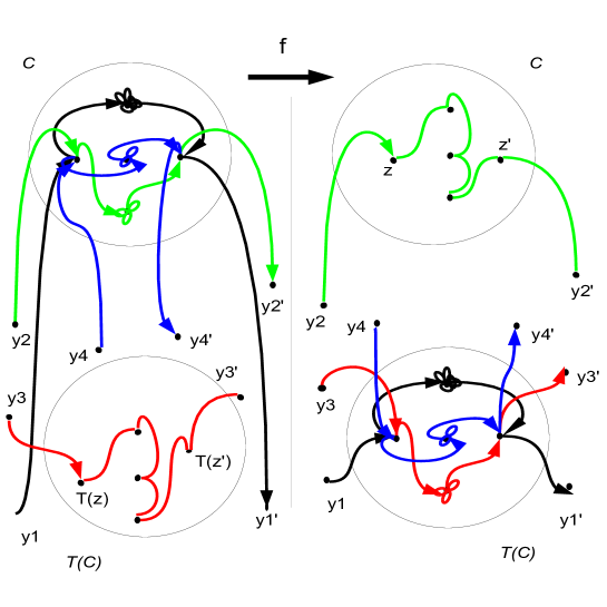
Figure 1: Action of $f$ on proper loops.

Remark 5.5

One implication of the key feature of $\varphi_{n,m}$, namely that $(\eta_{p},\varphi_{n,m}(\eta_{p}))\in E_{n,m}$, is that a trip $(y,{\cal{T}}(z))$ or $({\cal{T}}(z^{\prime}),y^{\prime})$ is invariant under $f_{p}$. Note that in Figure 1, $(y_{3},{\cal{T}}(z))$ and $({\cal{T}}(z^{\prime}),y_{3}^{\prime})$ are invariant, whereas $(y_{1},z)$ becomes $(y_{1},{\cal{T}}(z))$ and fortunately $|y_{1}-{\cal{T}}(z)|\leq|y_{1}-z|$ on the drawing.

Note that $f_{p}$ satisfies (5.4). Indeed, if we call $z_{p}$ the substring of $z$ made up of only sites represented in (5.12), and $f_{p}(z_{p})$ the substring of $f_{p}(z)$ made up of only sites represented in (5.13), we have $l_{f_{p}(z_{p})}(x)=l_{z_{p}}(x)$ for $x\in\Lambda\backslash{\cal{C}}$,

$$\forall x\in{\cal{C}},\quad l_{f_{p}(z_{p})}({\cal{T}}(x))=l_{z_{p}}(x),\quad\text{and}\quad l_{f_{p}(z_{p})}(x)=l_{z_{p}}({\cal{T}}(x)).$$ (5.14)

Now, we estimate the cost of going from $z_{p}$ to $f_{p}(z_{p})$. We consider encaged loops as described in Section 4.2. The purpose of having defined types, and of having encaged loops, is the following two simple observations, which we deduce from (4.15) in Remark 4.7.

$$\text{(i)}\qquad\text{Weight}(\tilde{\cal{L}}_{1})\text{Weight}({\cal{L}}_{2})=\text{Weight}({\cal{T}}^{-1}(\tilde{\cal{L}}_{1}))\text{Weight}({\cal{T}}({\cal{L}}_{2})),$$ (5.15)

and, if $p=(z,z^{\prime})\in{\cal{C}}^{2}$

$$\text{(ii)}\qquad\text{Weight}({\cal{L}}_{1})=\frac{P_{y_{1}}\left({S_{T}=z}\right)}{P_{y_{1}}\left({S_{T}={\cal{T}}(z)}\right)}\frac{P_{z^{\prime}}\left({S_{T}=y^{\prime}_{1}}\right)}{P_{{\cal{T}}(z^{\prime})}\left({S_{T}=y^{\prime}_{1}}\right)}\quad\text{Weight}({\cal{T}}({\cal{L}}_{1})),$$ (5.16)

and a similar equality linking $\text{Weight}({\cal{L}}_{3})$ and $\text{Weight}({\cal{T}}({\cal{L}}_{3}))$. Thus, the cost of transformation (5.13) is $C_{T}^{4}$, where $C_{T}$ appears in Lemma 4.10, since only 2 entering trips and 2 exiting trips have been wired differently.

Now, for any ${\bf z}\in{\cal{E}}({\bf k})$, the number of loops which undergo a transformation is less than the total number of loops, which is bounded by $\epsilon{\sqrt{n}}$. The maximum cost (maximum over ${\bf z}\in{\cal{E}}({\bf k})$) of such an operation is $2C_{T}$ to the power $\epsilon{\sqrt{n}}$.

The case (rare but possible) where $\nu(p)<\nu(\tilde{p})$ has to be dealt with differently. Indeed, for an arbitrary cluster ${\cal{C}}^{\prime}$, we cannot transform a trip between ${\cal{C}}^{\prime}$ and $\tilde{\cal{C}}$ into a trip between ${\cal{C}}^{\prime}$ and ${\cal{C}}$ at a constant cost, since $\text{dist}({\cal{C}}^{\prime},\tilde{\cal{C}})$ might be much smaller than $\text{dist}({\cal{C}}^{\prime},{\cal{C}})$.

We propose that $f_{p}$ performs the following changes:

• Act with ${\cal{T}}$ on all ${\cal{C}}$-loops of type $p$.

• Act with ${\cal{T}}^{-1}$ only on the first $\nu(p)$ $\tilde{\cal{C}}$-loops of type $\tilde{p}$.

• Interchange the position of the $\nu(p)$ first ${\cal{C}}$-loops with $\nu(p)$ first $\tilde{\cal{C}}$-loops.

For instance, in the following example, ${\bf z}$ has three $\tilde{\cal{C}}$-loops $\tilde{\cal{L}}_{1},\tilde{\cal{L}}_{2}$ and $\tilde{\cal{L}}_{3}$ and one ${\cal{C}}$-loop ${\cal{L}}_{1}$,

$${\bf z}:\dots y_{1}\tilde{\cal{L}}_{1}y_{1}^{\prime}\dots y_{2}{\cal{L}}_{1}y_{2}^{\prime}\dots y_{3}\tilde{\cal{L}}_{2}y_{3}^{\prime}\dots y_{4}\tilde{\cal{L}}_{3}y_{4}^{\prime}.$$

$\nu(p)=1<\nu(\tilde{p})=3$, and we have

$${\bf z}:\longrightarrow f_{p}({\bf z}):\dots y_{1}{\cal{T}}({\cal{L}}_{1})y_{1}^{\prime}\dots y_{2}{\cal{T}}^{-1}(\tilde{\cal{L}}_{1})y_{2}^{\prime}\dots y_{3}\tilde{\cal{L}}_{2}y_{3}^{\prime}\dots y_{4}\tilde{\cal{L}}_{3}y_{4}^{\prime}.$$ (5.17)

In so doing, note that the cost is 1, but instead of (5.14), we have

$$\forall x\in{\cal{C}},\quad l_{f_{p}(z_{p})}({\cal{T}}(x))\geq l_{z_{p}}(x),\quad\text{and}\quad\forall x\in{\cal{C}},\quad l_{f_{p}(z_{p})}(x)\leq l_{z_{p}}({\cal{T}}(x)).$$ (5.18)

Also, we have brought a multiplicity of pre-images. Indeed, note that the final circuit of (5.17) could have been obtained, following the rule of (5.13), by a circuit ${\bf z^{\prime}}$ where $\nu(p)\geq\nu(\tilde{p})$:

$${\bf z^{\prime}}:\dots y_{1}{\cal{L}}_{1}y_{1}^{\prime}\dots y_{2}{\cal{T}}^{-1}({\cal{L}}_{2}^{\prime})y_{2}^{\prime}\dots y_{3}\tilde{\cal{L}}_{1}y_{3}^{\prime}\dots y_{4}{\cal{T}}^{-1}({\cal{L}}_{3}^{\prime})y_{4}^{\prime}\dots\longrightarrow f_{p}({\bf z}).$$ (5.19)

Also, $f_{p}$ maps a proper loop into a proper loop, and a pre-image under $f_{p}$ has either $\nu(p)\geq\nu(\tilde{p})$ or $\nu(p)<\nu(\tilde{p})$, and so only two possible pre-images. Since this is true for any type, an upper bound on the number of pre-images of the composition of all $f_{p}$, is bounded by 2 to the power $|{\cal{C}}|^{2}$ (which is the number of types). Since ${\cal{C}}\subset\Lambda$ whose volume is independent of $n$, the multiplicity is innocuous in this case.

5.3 Improper Loops.

In this section, we deal with trips in ${\cal{C}}\times\tilde{\cal{C}}\cup\tilde{\cal{C}}\times{\cal{C}}$. The notion of type is not useful here. We call $f_{i}$ the action of $f$ on improper loops.

To grasp the need to distinguish proper loops from improper loops, assume that we have a trip from a ${\cal{T}}({\cal{C}})$-loop to a ${\cal{C}}$-loop. If we could allow the ${\cal{C}}$-loop to become a ${\cal{T}}({\cal{C}})$-loop, we could reach a situation with two successive ${\cal{T}}({\cal{C}})$-loops linked with no trip. They would merge into one ${\cal{T}}({\cal{C}})$-loop by our definition 4.3. This may increase dramatically the number of pre-images of a given $f({\bf z})$, violating (5.5).

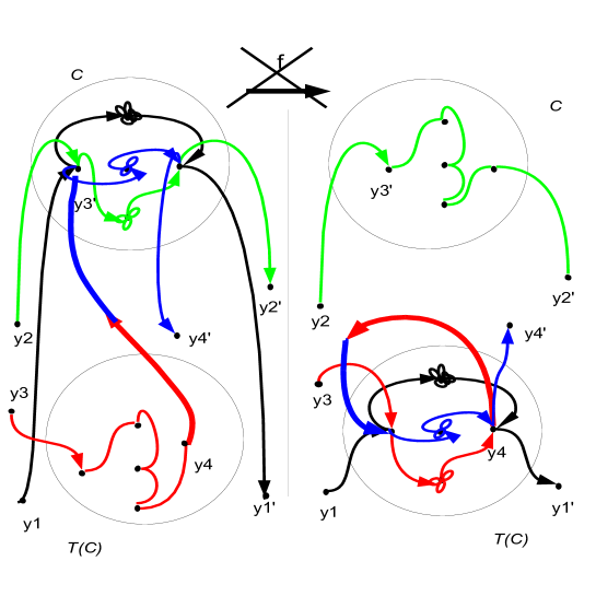
Figure 2: Red and blue loops merging.

We illustrate this with a concrete example drawn in Figure 2, below. We have considered the same example as in (5.12), but now there is a trip between $\tilde{\cal{L}}_{1}$ to ${\cal{L}}_{3}$, so that $y^{\prime}_{3}$ is in loop ${\cal{L}}_{3}$ whereas $y_{4}\in\tilde{\cal{L}}_{1}$, as shown in Figure 2. If we where to apply the algorithm of Section 5.2, we would obtain the image shown on the right hand side of in Figure 2. There, the loops ${\cal{T}}({\cal{L}}_{2})$ and ${\cal{T}}({\cal{L}}_{3})$ (that we obtain in (5.13)) would have to merge.

Consider first a circuit with a string of successive improper loops of type $p$, such that the number of ${\cal{C}}$-loops matches the number of $\tilde{\cal{C}}$-loops. For instance, assume that the $i$-th $\tilde{\cal{C}}$-loop is improper and followed by the $j$-th ${\cal{C}}$-loop, and so forth. For definiteness, assume that ${\bf z}$ contains $z_{i}$ ($i$ for improper) with

$$z_{i}:=y_{1}\tilde{\cal{L}}(i){\cal{L}}(j)\dots\tilde{\cal{L}}(i+k){\cal{L}}(j+k)y^{\prime}_{1},\quad\text{with}\ k\geq 0,\ \text{ and}\quad y_{1},y^{\prime}_{1}\not\in{\cal{C}}\cup\tilde{\cal{C}}.$$ (5.20)

Our purpose is to transform such a sequence of alternating ${\cal{C}}$-$\tilde{\cal{C}}$ loops into a similar alternating sequence, such that $f_{i}(z_{i})$ satisfies (5.4), (5.5) and (5.6).

One constraint is that we cannot replace the entering trip, and exiting trip in general, which in turn fixes the order of visits to ${\cal{C}}$ and $\tilde{\cal{C}}$. Indeed, as in the previous section, if $p=(z,z^{\prime})$ and $|y_{1}-{\cal{T}}(z)|\ll|y_{1}-z|$, then we cannot map the trip $(y_{1},{\cal{T}}(z))$ to $(y_{1},z)$ at a small cost. We propose to following map

$$f_{i}(z_{i}):=y_{1}{\cal{T}}({\cal{L}}(j)){\cal{T}}^{-1}(\tilde{\cal{L}}(i))\dots\cal{T}({\cal{L}}(j+k)){\cal{T}}^{-1}({\cal{L}}(i+k))y^{\prime}_{1}$$ (5.21)

Note that (5.14) holds. With an abuse of notations we represent the probability associated with $f_{i}(z_{i})$, as

$$\text{Weight}(f_{i}(z_{i})):=\prod_{l=0}^{k-1}\text{Weight}(\tilde{\cal{L}}(i+l))\text{Weight}({\cal{L}}(j+l)),$$ (5.22)

even though we mean now that the trips joining successives journeys between ${\cal{C}}$-$\tilde{\cal{C}}$ or $\tilde{\cal{C}}$-${\cal{C}}$are counted only once. Thus, the estimates we need concern trips joining improper loops together, in addition to the first entering and the last exiting trip from $\gamma$. These estimates are the content of Lemma 4.12. The cost $\text{Weight}(z_{i})/\text{Weight}(f_{i}(z_{i}))$ is bounded by $C_{I}^{2(k+1)+1}$, where $k+1$ is the number of successive blocks of $\tilde{\cal{C}}$-${\cal{C}}$ loops. Since the total number of improper loops of all types is bounded by $\epsilon{\sqrt{n}}$, the total cost is negligible in our order of asymptotics.

The case where the number of ${\cal{C}}$ and $\tilde{\cal{C}}$-loops does not match is trickier. First, assume that we deal with

$$z_{i}:=y_{1}{\cal{L}}(i)\tilde{\cal{L}}(j)\dots\cal{L}(i+k)y^{\prime}_{1}.$$ (5.23)

Here, we have no choice but to replace $z_{i}$ with

$$f_{i}(z_{i}):=y_{1}{\cal{T}}({\cal{L}}(i)){\cal{T}}^{-1}({\cal{L}}(j))\dots\cal{T}({\cal{L}}(i+k))y^{\prime}_{1}.$$ (5.24)

Note that (5.18) holds.

Lastly, consider the case with more $\tilde{\cal{C}}$-loops. For instance,

$$z_{i}:=y_{1}\tilde{\cal{L}}(i){\cal{L}}(j)\tilde{\cal{L}}(i+1)\dots\cal{L}(j+k-1)\tilde{\cal{L}}(i+k)y^{\prime}_{1}.$$ (5.25)

For reasons already mentioned, we cannot map the first $\tilde{\cal{C}}$-loop into a ${\cal{C}}$-loop. We propose to keep the first loop unchanged, and act on the remaining loops, in the following way

$$f_{i}(z_{i}):=y_{1}\tilde{\cal{L}}(i){\cal{T}}^{-1}(\tilde{\cal{L}}_{i+1}){\cal{T}}({\cal{L}}(j))\dots\cal{T}^{-1}(\tilde{\cal{L}}_{i+k}){\cal{T}}({\cal{L}}(j+k-1))y^{\prime}_{1}.$$ (5.26)

Here, as in (5.17), (5.18) holds, and this choice brings a multiplicity of pre-images. Indeed, $f_{i}(z_{i})$ could have come from

$$z_{i}^{\prime}:=y_{1}{\cal{T}}^{-1}(\tilde{\cal{L}}(i))\tilde{\cal{L}}(i+1){\cal{L}}(j)\dots\tilde{\cal{L}}_{i+k}{\cal{T}}({\cal{L}}(j+k-1)y^{\prime}_{1}\longrightarrow f_{i}(z_{i}).$$

So, in estimating the number of pre-images of a circuit, we find that it is at most 2 to the power of the number of improper loops. Now, the maximum number of improper loops is $\epsilon{\sqrt{n}}$. Also, the cost of transforming all improper loops is uniformly bounded by $C_{I}$ to the power $\epsilon{\sqrt{n}}$.

6 Renormalizing Time.

In this section, we show the following result.

Proposition 6.1

For any finite domain $\tilde{\Lambda}\subset{\mathbb{Z}}^{d}$, there are positive constants $\alpha_{0}$, $\gamma$, such that for any large integer $n$, there is a sequence ${\bf k_{n}^{*}}=\left\{{k_{n}^{*}(z),\ z\in\tilde{\Lambda}}\right\}$ with

$$\sum_{z\in\tilde{\Lambda}}k_{n}^{*}(z)\leq n,\quad\left\{{k_{n}^{*}(z)\in[\frac{\sqrt{n}}{A},A\sqrt{n}],\ z\in\tilde{\Lambda}}\right\},\quad\text{and}\quad\sum_{z\in\tilde{\Lambda}}k_{n}^{*}(z)^{2}\geq n\xi,$$ (6.1)

such that for any $\alpha>\alpha_{0}$

$$P_{0}\left({||\hbox{1\hskip-3.0ptI}_{\tilde{\Lambda}}l_{\infty}||_{2}^{2}\geq n\xi,\quad\tilde{\Lambda}\subset{\cal{D}}_{\infty}(A,\sqrt{n})}\right)\leq n^{\gamma}P_{0}\left({l_{\lfloor\alpha\sqrt{n}\rfloor}|_{\tilde{\Lambda}}={\bf k_{n}^{*}},\ S_{\lfloor\alpha\sqrt{n}\rfloor}=0}\right).$$ (6.2)

Proof.  We first use a rough upper bound

$$P_{0}\left({||\hbox{1\hskip-3.0ptI}_{\tilde{\Lambda}}l_{\infty}||_{2}^{2}\geq n\xi,\tilde{\Lambda}\subset{\cal{D}}_{\infty}(A,\sqrt{n})}\right)\leq\big{|}\left\{{{\bf k_{n}}\in[\frac{\sqrt{n}}{A},A{\sqrt{n}}]^{\tilde{\Lambda}}}\right\}\big{|}\max_{{\bf k_{n}}\text{ in }(\ref{seq-time})}P(l_{\infty}|_{\tilde{\Lambda}}={\bf k_{n}}).$$ (6.3)

We choose a sequence ${\bf k_{n}^{*}}$ which maximizes the last term in (6.3). Then, we decompose $\left\{{l_{\infty}|_{\tilde{\Lambda}}={\bf k_{n}^{*}}}\right\}$ into all possible circuits in a manner similar to the circuit decomposition of Section 4: We set $\nu=\sum_{\tilde{\Lambda}}k_{n}^{*}(x)$ (and $\nu\leq|\tilde{\Lambda}|A\sqrt{n}$), and

$${\cal{E}}^{*}=\left\{{{\bf z}=(z(1),\dots,z(\nu))\in\tilde{\Lambda}^{\nu}:\ l_{{\bf z}}(x)=k_{n}^{*}(x),\ \forall x\in\tilde{\Lambda}}\right\}.$$ (6.4)

Then, if $T=\inf\left\{{n\geq 0:\ S_{n}\in\tilde{\Lambda}}\right\}$, (and $z(0)=0$)

$$P_{0}(l_{\infty}|_{\tilde{\Lambda}}={\bf k_{n}^{*}})=\sum_{{\bf z}\in{\cal{E}}^{*}}\prod_{i=0}^{\nu-1}P_{z(i)}\left({\tilde{T}(z({i+1}))=T<\infty}\right)P_{z(\nu)}(T=\infty).$$ (6.5)

For a fixed ${\bf z}\in{\cal{E}}^{*}$, we call $\tau^{(i)}$ the duration of the flight from $z(i-1)$ and $z(i)$ which avoids other sites of $\tilde{\Lambda}$. Thus, $\tau^{(1)}\overset{\text{law}}{=}\tilde{T}(z(1))\hbox{1\hskip-3.0ptI}\{\tilde{T}(z(1))=T\}$, when restricting on the values $\left\{{1,2,\dots}\right\}$, and by induction

$$\tau^{(i)}\overset{\text{law}}{=}\tilde{T}(z(i))\circ\theta_{\tau^{(i-1)}}\hbox{1\hskip-3.0ptI}\left\{{\tilde{T}(z(i))\circ\theta_{\tau^{(i-1)}}=T\circ\theta_{\tau^{(i-1)}}}\right\}$$ (6.6)

If ${\mathsf{T}}({\bf z})=\left\{{0<\tau^{(i)}<\infty,\forall i=1,\dots,\nu}\right\}$, we have

$$P_{0}({\mathsf{T}}({\bf z}))=\prod_{i=0}^{\nu-1}P_{z(i)}\left({\tilde{T}(z({i+1}))=T<\infty}\right).$$ (6.7)

Now, we fix ${\bf z}\in{\cal{E}}^{*}$ such that $P_{0}({\mathsf{T}}({\bf z}))>0$, and we fix $i<\nu$. For ease of notations, we rename $x=z(i-1)$ and $y=z({i})$. Now, note that $\left\{{0<\tau^{(i)}<\infty}\right\}$ contributes to (6.7) if $P_{x}(S_{T}=y)>0$, or in other words, if there is at least one path going from $x$ to $y$ avoiding other sites of $\tilde{\Lambda}$. Since $\tilde{\Lambda}$ has finite diameter, we can choose a finite length self-avoiding paths, and have

$$P_{x}\left({T(y)<\tilde{T}(x)}\right)\geq c_{\Lambda}(x,y):=P_{x}(S_{T}=y,T<\infty)>c_{\Lambda}>0,$$ (6.8)

where $c_{\Lambda}$ is the minimum of $c_{\Lambda}(z,z^{\prime})$ over all $z,z^{\prime}\in\tilde{\Lambda}$ with $c_{\Lambda}(z,z^{\prime})>0$. Now, note that, when $S_{0}=y$

$$\tilde{T}(y)\hbox{1\hskip-3.0ptI}_{T(x)<\tilde{T}(y)<\infty}\leq\tilde{T}(y)\hbox{1\hskip-3.0ptI}_{\tilde{T}(y)<\infty}.$$ (6.9)

Thus,

$$\begin{split}E_{y}\left[{\tilde{T}(y)\hbox{1\hskip-3.0ptI}_{\tilde{T}(y)<\infty}}\right]&\geq E_{y}\left[{\hbox{1\hskip-3.0ptI}_{T(x)<\tilde{T}(y)<\infty}\left({\tilde{T}(y)\circ\theta_{T(x)}+T(x)}\right)}\right]\\ &=E_{y}\left[{\hbox{1\hskip-3.0ptI}_{T(x)<\tilde{T}(y)<\infty}T(x)}\right]+E_{y}\left[{\hbox{1\hskip-3.0ptI}_{T(x)<\tilde{T}(y)<\infty}\tilde{T}(y)\circ\theta_{T(x)}}\right].\end{split}$$ (6.10)

Now, by the strong Markov’s property

$$E_{y}\left[{\tilde{T}(y)\hbox{1\hskip-3.0ptI}_{\tilde{T}(y)<\infty}}\right]\geq P_{y}\left({T(x)<\tilde{T}(y)}\right)E_{x}\left[{T(y)\hbox{1\hskip-3.0ptI}_{T(y)<\infty}}\right].$$ (6.11)

By using translation invariance of the walk and (6.11), we obtain

$$E_{x}\left[{T(y)\hbox{1\hskip-3.0ptI}_{T(y)=T<\infty}}\right]\leq E_{x}\left[{T(y)\hbox{1\hskip-3.0ptI}_{T(y)<\infty}}\right]\leq\frac{E_{0}\left[{\tilde{T}(0)\hbox{1\hskip-3.0ptI}_{\tilde{T}(0)<\infty}}\right]}{P_{y}\left({T(x)<\tilde{T}(y)}\right)}.$$ (6.12)

Now, it is well known that there is a constant $c_{d}>0$ such that for any integer $k$, $P_{0}(\tilde{T}(0)=k)\leq c_{d}/k^{\frac{d}{2}}$, which implies that $E_{0}\left[{\tilde{T}(0)\hbox{1\hskip-3.0ptI}_{\tilde{T}(0)<\infty}}\right]<\infty$ in $d\geq 5$, and

$$E_{x}\left[{T(y)|T(y)=T<\infty}\right] = \frac{E_{x}\left[{T(y)\hbox{1\hskip-3.0ptI}_{T(y)=T<\infty}}\right]}{P_{x}(T(y)=T<\infty)}$$ (6.13)

$$\leq \frac{E_{0}\left[{\tilde{T}(0)\hbox{1\hskip-3.0ptI}_{\tilde{T}(0)<\infty}}\right]}{P_{x}(T(y)=T<\infty)P_{y}(T(x)<\tilde{T}(y))}$$ (6.13)

$$\leq \frac{E_{0}\left[{\tilde{T}(0)\hbox{1\hskip-3.0ptI}_{\tilde{T}(0)<\infty}}\right]}{c_{\Lambda}^{2}}.$$ (6.13)

When translating (6.13) in terms of the $\left\{{\tau^{(i)}}\right\}$, we obtain for any $\beta>0$

$$P\left({\sum_{i=1}^{\nu}\tau^{(i)}>\beta\nu\big{|}{\mathsf{T}}({\bf z})}\right)\leq\frac{E_{0}\left[{\sum_{i=1}^{\nu}\tau^{(i)}|{\mathsf{T}}({\bf z})}\right]}{\beta\nu}\leq\frac{E_{0}\left[{\tilde{T}(0)\hbox{1\hskip-3.0ptI}_{\tilde{T}(0)<\infty}}\right]}{c_{\Lambda}^{2}}\times\frac{1}{\beta}.$$ (6.14)

Thus, we can choose $\beta_{0}$ large enough (independent of ${\bf z}$) so that

$$P_{0}\left({\sum_{i=1}^{\nu}\tau^{(i)}>\beta_{0}\nu|{\mathsf{T}}({\bf z})}\right)\leq\frac{1}{2}.$$ (6.15)

We use now

$$P_{0}({\mathsf{T}}({\bf z}))=P_{0}\left({\sum_{i=1}^{\nu}\tau^{(i)}>\beta_{0}\nu|{\mathsf{T}}({\bf z})}\right)P_{0}({\mathsf{T}}({\bf z}))+P_{0}\left({\sum_{i=1}^{\nu}\tau^{(i)}\leq\beta_{0}\nu|{\mathsf{T}}({\bf z})}\right)P_{0}({\mathsf{T}}({\bf z})),$$

to conclude that

$$P_{0}({\mathsf{T}}({\bf z}))\leq 2P_{0}\left({\{\sum_{i=1}^{\nu}\tau^{(i)}\leq\beta_{0}\nu\}\cap{\mathsf{T}}({\bf z})}\right).$$ (6.16)

Now, there is $\alpha_{0}$ such that $\beta_{0}\nu\leq\alpha_{0}\sqrt{n}$. Also, note that there is $n_{0}$ such that for any $z(\nu)\in\tilde{\Lambda}$, there is a path of length $n_{0}$ joining $z(\nu)$ to 0. Now, fix $\alpha>2\alpha_{0}$, take $n$ large enough so that $\lfloor\alpha\sqrt{n}\rfloor\geq\lfloor\alpha_{0}\sqrt{n}\rfloor+n_{0}$, and use classical estimates on return probabilities, to obtain that for a constant $C_{d}$

$$P_{0}({\mathsf{T}}({\bf z}))\leq C_{d}(\alpha n)^{d/2}\!\!\sum_{\nu\leq k\leq\beta_{0}\nu}\!\!P_{0}\big{(}\{\sum_{i=1}^{\nu}\tau^{(i)}=k\}\cap{\mathsf{T}}({\bf z})\big{)}P_{z(\nu)}(S_{n_{0}}=0)P_{0}(S_{\lfloor\alpha n\rfloor-(k+n_{0})}=0).$$ (6.17)

After summing over $z\in{\cal{E}}^{*}$, we obtain for any $\alpha>2\alpha_{0}$

$$\sum_{z\in{\cal{E}}^{*}}P_{0}({\mathsf{T}}({\bf z}))\leq C_{d}(\alpha n)^{d/2}P_{0}\left({||\hbox{1\hskip-3.0ptI}_{\tilde{\Lambda}}l_{\lfloor\alpha\sqrt{n}\rfloor}||_{2}^{2}\geq n\xi,S_{\lfloor\alpha\sqrt{n}\rfloor}=0}\right).$$ (6.18)

Note that another power of $n$ arises from the term in (6.3) yielding the desired result.  

7 Existence of a Limit.

We keep notations of Section 6. We reformulate Proposition 6.1 as follows. For any finite domain $\tilde{\Lambda}\subset{\mathbb{Z}}^{d}$, there are positive constants $\alpha_{0}$, $\gamma$, such that for any $\alpha>\alpha_{0}$, and $n$ large

$$P_{0}\left({||\hbox{1\hskip-3.0ptI}_{\tilde{\Lambda}}l_{\infty}||_{2}^{2}\geq n\xi,\quad\tilde{\Lambda}\subset{\cal{D}}_{\infty}(A,\sqrt{n})}\right)\leq n^{\gamma}P_{0}\left({||\hbox{1\hskip-3.0ptI}_{\tilde{\Lambda}}l_{\lfloor\alpha\sqrt{n}\rfloor}||_{2}\geq\sqrt{n\xi},\ S_{\lfloor\alpha\sqrt{n}\rfloor}=0}\right).$$ (7.1)

Thus, (7.1) is the starting point in this section.

7.1 A Subadditive Argument.

We consider a fixed region $\Lambda\ni 0$, and first show the following lemma.

Lemma 7.1

Let $q>1$. For any $\xi>0$ and $\Lambda$ finite subset of ${\mathbb{Z}}^{d}$, the following limit exists

$$\lim_{n\to\infty}\frac{\log(P_{0}(||\hbox{1\hskip-3.0ptI}_{\Lambda}l_{n}||_{q}\geq n\xi,\ S_{n}=0))}{n}=-I(\xi,\Lambda).$$ (7.2)

Proof.

We fix two integers $K$ and $n$, with $K$ to be taken first to infinity. Let $m,r$ be integers such that $K=mn+r$, and $0\leq r<n$. The phenomenon behind the subadditive arguement is that

$${\cal{A}}_{K}(\xi,\Lambda)=\left\{{||\hbox{1\hskip-3.0ptI}_{\Lambda}l_{K}||_{q}\geq K\xi,\ S_{K}=0}\right\}$$ (7.3)

is built by concatenating the ${\it same}$ optimal scenario realizing ${\cal{A}}_{n}(\xi,\Lambda)$ on $m$ consecutive time-periods of length $n$, and one last time-period of length $r$ where the scenario is necessarly special and its cost innocuous. The crucial independence between the different periods is obtained as we force the walk to return to the origin at the end of each time period.

Our first step is to exhibit an optimal strategy realizing ${\cal{A}}_{n}(\xi,\Lambda)$. By optimizing over a finite number of variables $\{k_{n}(x),x\in\Lambda\}$ satisfying

$$\sum_{x\in\Lambda}k_{n}(x)^{q}\geq(n\xi)^{q},\quad\text{and}\quad\sum_{x\in\Lambda}k_{n}(x)\leq n,$$ (7.4)

there is a sequence ${\bf k_{n}^{*}}:=\left\{{k_{n}^{*}(x),x\in\Lambda}\right\}$ and $\gamma>0$ (both depend on $\Lambda$) such that

$$P_{0}\left({{\cal{A}}_{n}(\xi,\Lambda)}\right)\leq n^{\gamma}P_{0}\left({{\cal{A}}_{n}^{*}(\xi,\Lambda)}\right),,\quad\text{with}\quad{\cal{A}}_{n}^{*}(\xi,\Lambda)=\left\{{l_{n}|_{\Lambda}={\bf k_{n}^{*}},\ S_{n}=0}\right\}.$$ (7.5)

Let $z^{*}\in\Lambda$, be the site where ${\bf k_{n}^{*}}$ reaches its maximum. We start witht the case $z^{*}=0$, and postpone the case $z^{*}\not=0$ to Remark 7.2. When $z^{*}=0$, for any integer $r$, we call

$${\mathcal{R}}_{r}=\left\{{l_{r}(0)=r}\right\},\quad\text{and note that}\quad P_{0}({\mathcal{R}}_{r})=P_{0}(S_{1}=0)^{r-1}>0.$$ (7.6)

Now, denote by ${\cal{A}}_{n}^{(1)},\dots,{\cal{A}}_{n}^{(m)}$ $m$ independent copies of ${\cal{A}}_{n}^{*}(\xi,\Lambda)$ which we realize on the successive increments of the random walk

$$\forall i=1,\dots,m,\quad{\cal{A}}_{n}^{(i)}=\left\{{l_{[(i-1)n,in[}|_{\Lambda}={\bf k_{n}^{*}},\ S_{in}=0}\right\}.$$

Make a copy of ${\mathcal{R}}_{r}$ independent of ${\cal{A}}_{n}^{(1)},\dots,{\cal{A}}_{n}^{(m)}$, by using increments after time $nm$: that is ${\mathcal{R}}_{r}=\{S_{j}=0,\ \forall j\in[nm,K[\}$. Note that by independence

$$\begin{split}P_{0}\left({{\cal{A}}_{n}(\xi,\Lambda)}\right)^{m}P_{0}({\mathcal{R}}_{r})\leq&(n^{\gamma})^{m}P_{0}({\cal{A}}_{n}^{(1)})\dots P_{0}({\cal{A}}_{n}^{(m)})P_{0}({\mathcal{R}}_{r})\\ \leq&(n^{\gamma})^{m}P_{0}(\bigcap_{j=1}^{m}{\cal{A}}_{n}^{(j)})\cap{\mathcal{R}}_{r}).\end{split}$$ (7.7)

Now, the local times is positive, so that

$$\begin{split}\bigcap_{i=1}^{m}&\left\{{l_{[(i-1)n,in[}|_{\Lambda}={\bf k_{n}^{*}},\ S_{in}=0}\right\}\cap\left\{{l_{[mn,K[}(0)=r}\right\}\\ &\subset\left\{{\sum_{x\in\Lambda}\left[{\sum_{i=1}^{m}l_{[(i-1)n,in[}(x)+\ l_{[mn,K[}(x)}\right]^{q}\geq\sum_{x\in\Lambda}\left({mk_{n}^{*}(x)+r\delta_{0}(x)}\right)^{q},S_{K}=0}\right\}.\end{split}$$

At this point, observe the following fact whose simple inductive proof we omit: for $q>1$, and for $\varphi$ and $\psi$ are positive functions on $\Lambda$, and for $z^{*}\in\Lambda$, $\varphi(z^{*})=\max\varphi$, then

$$(\varphi(z^{*})+\sum_{z\in\Lambda}\psi(z))^{q}+\sum_{z\not=z^{*}}\varphi(z)^{q}\geq\sum_{z\in\Lambda}\left({\varphi(z)+\psi(z)}\right)^{q}.$$ (7.8)

(7.8) implies that for any integer $m$

$$\sum_{x\in\Lambda}\left({mk_{n}^{*}(x)+r\delta_{z^{*}}(x)}\right)^{q} \geq \sum_{x\in\Lambda}\left({mk_{n}^{*}(x)+\frac{r}{n}k_{n}^{*}(x)}\right)^{q}$$ (7.9)

$$= (m+\frac{r}{n})^{q}\sum_{x\in\Lambda}k_{n}^{*}(x)^{q}\geq(mn+r)^{q}\xi^{q}=(K\xi)^{q}.$$ (7.9)

Using (7.9), (7.7) yields

$$P_{0}\left({{\cal{A}}_{n}(\xi,\Lambda)}\right)^{m}P_{0}({\mathcal{R}}_{r})\leq(n^{\gamma})^{m}P_{0}\left({||\hbox{1\hskip-3.0ptI}_{\Lambda}l_{K}||_{q}\geq K\xi,\ S_{K}=0}\right)\leq(n^{\gamma})^{m}P_{0}\left({{\cal{A}}_{K}(\xi,\Lambda)}\right).$$ (7.10)

We now take the logarithm on each side of (7.7)

$$\frac{nm}{nm+r}\frac{\log(P_{0}({\cal{A}}_{n}(\xi,\Lambda)))}{n}+\frac{\log(P_{0}({\mathcal{R}}_{r}))}{K}\leq\frac{m(\log(n^{\gamma}))}{nm+r}+\frac{\log(P_{0}({\cal{A}}_{K}(\xi,\Lambda)))}{K}.$$ (7.11)

We take now the limit $K\to\infty$ while $n$ is kept fixed (e.g. $m\to\infty$) so that

$$\frac{\log(P_{0}({\cal{A}}_{n}(\xi,\Lambda)))}{n}\leq\frac{\log(n^{\gamma})}{n}+\liminf_{K\to\infty}\frac{\log(P_{0}({\cal{A}}_{K}(\xi,\Lambda)))}{K}.$$ (7.12)

By taking the limit sup in (7.12) as $n\to\infty$, we conclude that the limit in (7.2) exists.

Remark 7.2

We treat here the case $z^{*}\not=0$. In this case, we cannot consider ${\mathcal{R}}_{r}$ since to use (7.8), we would need the walk to start on site $z^{*}$, whereas each period of length $n$ sees the walk returning to the origin. Note that this problem is related to the strategy on a single time-period of length $r$. The remedy is simple: we insert a period of length $r$ into the first time-period of length $n$ at the first time the walk hits $z^{*}$; then, the walk stays at $z^{*}$ during $r-1$ steps. In other words, let $\tau^{*}=\inf\{n\geq 0:\ S_{n}=z^{*}\}$, ${\mathcal{R}}_{r}^{*}=\{l_{r}(z^{*})=r\}$ and note that

$$\begin{split}P_{0}({\cal{A}}_{n}^{(1)})P_{z^{*}}({\mathcal{R}}_{r}^{*})=&\sum_{i=1}^{n}P_{0}({\cal{A}}_{n}^{(1)},\tau^{*}=i)P_{z^{*}}(l_{r}(z^{*})=r)\\ \leq&P_{0}\left({l_{[0,n+r[}|_{\Lambda}={\bf k_{n}^{*}}+r\delta_{z^{*}}}\right).\end{split}$$ (7.13)

Note that $P_{z^{*}}({\mathcal{R}}_{r}^{*})=P_{0}({\mathcal{R}}_{r})$, and

$$\bigcap_{j=1}^{m}{\cal{A}}_{n}^{(j)}\subset\left\{{\sum_{x\in\Lambda}\left[{l_{[0,n+r[}(x)+\sum_{i=2}^{m}l_{[(i-1)n,in[}(x)}\right]^{q}\geq\sum_{x\in\Lambda}\left({mk_{n}^{*}(x)+r\delta_{z^{*}}(x)}\right)^{q},S_{K}=0}\right\}.$$

We can now resume the proof of the case $z^{*}=0$ at step (7.9).

 

7.2 Lower Bound in Proposition 1.6.

We prove here the lower bound of (1.16). Call $t_{n}$ be the integer part of $\alpha\sqrt{n}$, and consider the following scenario

$${\cal{S}}_{n}(\Lambda,\alpha,\epsilon):=\left\{{||\hbox{1\hskip-3.0ptI}_{\Lambda}l_{[0,t_{n}[}||_{2}^{2}\geq n\xi(1+\epsilon),\ S_{t_{n}}=0}\right\}\cap\left\{{||l_{[t_{n},n[}||_{2}^{2}-E_{0}\left[{||l_{n}||_{2}^{2}}\right]\geq n\xi(1-\epsilon)}\right\},$$ (7.14)

Note that ${\cal{S}}_{n}(\Lambda,\alpha,\epsilon)\subset\{\overline{||l_{n}||_{2}^{2}}\geq n\xi\}$. Indeed, note that for any $\beta\geq 1$, and $a,b>0$ we have $a^{\beta}+b^{\beta}\leq(a+b)^{\beta}$. Thus, for any $x\in{\mathbb{Z}}^{d}$

$$l^{2}_{[0,t_{n}[}(x)+l^{2}_{[t_{n},n[}(x)\leq l^{2}_{n}(x),$$ (7.15)

and we obtain on ${\cal{S}}_{n}(\Lambda,\alpha,\epsilon)$

$$E_{0}\left[{||l_{n}||_{2}^{2}}\right]+n\xi\leq\sum_{x\in\Lambda}l^{2}_{[0,t_{n}[}(x)+\sum_{x\in{\mathbb{Z}}^{d}}l^{2}_{[t_{n},n[}(x)\leq||l_{n}||_{2}^{2}.$$ (7.16)

Note that $||\hbox{1\hskip-3.0ptI}_{\Lambda}l_{[0,t_{n}[}||_{2}$ and $S_{t_{n}}=0$ only depend on the increments of the random walk in the time period $[0,t_{n}[$, whereas $||l_{[t_{n},n[}||_{2}$ depends on the increments in $[t_{n},n[$. Thus,

$$\begin{split}P\left({{\cal{S}}_{n}(\Lambda,\alpha,\epsilon)}\right)=&P_{0}\left({||\hbox{1\hskip-3.0ptI}_{\Lambda}l_{[0,t_{n}[}||_{2}^{2}\geq n\xi(1+\epsilon),\ S_{t_{n}}=0}\right)\\ &\times P_{0}\left({||l_{[t_{n},n[}||_{2}^{2}-E_{0}\left[{||l_{n}||_{2}^{2}}\right]\geq n\xi(1-\epsilon)}\right).\end{split}$$ (7.17)

Now, since $\frac{1}{n}||l_{n}||_{2}^{2}$ converges in $L^{1}$ towards $\gamma_{d}$, we have $E_{0}[||l_{n}||_{2}^{2}]\leq n\gamma_{d}(1+\epsilon/2)$ for $n$ large enough, and we have

$$P_{0}\left({||l_{[t_{n},n[}||_{2}^{2}-E_{0}\left[{||l_{n}||_{2}^{2}}\right]\geq n\xi(1-\epsilon)}\right)\leq P_{0}\left({\frac{||l_{[0,n-t_{n}[}||_{2}^{2}}{n-t_{n}}\geq\frac{\gamma_{d}-\frac{\epsilon}{2}\xi}{1-\frac{t_{n}}{n}}}\right)\longrightarrow 1.$$ (7.18)

Remark 7.3

Note that for any $\Lambda$ finite subset of ${\mathbb{Z}}^{d}$, any $\beta>0$ and $\epsilon>0$ small, we have for $\chi<\zeta<1$, and $n$ large enough

$$\left\{{||\hbox{1\hskip-3.0ptI}_{\Lambda}l_{\lfloor\beta n^{\zeta}\rfloor}||_{\alpha^{*}}\geq\xi n^{\zeta}(1+\epsilon),\ S_{\lfloor\beta n^{\zeta}\rfloor}=0}\right\}\subset\left\{{||\hbox{1\hskip-3.0ptI}_{\bar{\cal{D}}_{n}(\chi)}l_{n}||_{\alpha^{*}}\geq\xi n^{\zeta}}\right\}.$$ (7.19)

7.3 Proof of Theorem 1.1

First, the upper bound of Proposition 1.6 follows after combining inequalities (3.2), (4.7), (5.1) and (7.1). The lower bound of Proposition 1.6 is shown in the previous section. Then, we invoke Lemma 7.1 with $q=2$, we take the logarithm on each sides of (1.16), we normalize by $\sqrt{n}$, and take the limit $n$ to infinity. We obtain that for any $\epsilon>0$, there are $\alpha_{\epsilon}$ and $\Lambda_{\epsilon}$ such that for $\Lambda,\Lambda^{\prime}\supset\Lambda_{\epsilon}$, and $\alpha,\alpha^{\prime}>\alpha_{\epsilon}$

$$\begin{split}-\alpha^{\prime}\ I\big{(}\frac{\sqrt{\xi(1+\epsilon)}}{\alpha^{\prime}}&,\Lambda^{\prime}\big{)}\leq\liminf_{n\to\infty}\frac{\log\left({P_{0}(\overline{||l_{n}||^{2}_{2}}\geq n\xi)}\right)}{\sqrt{n}}\\ &\leq\limsup_{n\to\infty}\frac{\log\left({P_{0}(\overline{||l_{n}||_{2}^{2}}\geq n\xi)}\right)}{\sqrt{n}}\leq-\alpha\ I\left({\frac{\sqrt{\xi(1-\epsilon)}}{\alpha},\Lambda}\right)+C\epsilon.\end{split}$$ (7.20)

By using (7.20), we obtain for any $\Lambda,\Lambda^{\prime}\supset\Lambda_{\epsilon}$, and $\alpha,\alpha^{\prime}>\alpha_{\epsilon}$

$$\frac{\alpha^{\prime}}{\sqrt{\xi(1+\epsilon)}}I\left({\frac{\sqrt{\xi(1+\epsilon)}}{\alpha^{\prime}},\Lambda^{\prime}}\right)\geq\sqrt{\frac{1-\epsilon}{1+\epsilon}}\frac{\alpha}{\sqrt{\xi(1-\epsilon)}}I\left({\frac{\sqrt{\xi(1-\epsilon)}}{\alpha},\Lambda}\right)-\frac{C\epsilon}{\sqrt{\xi(1+\epsilon)}}.$$ (7.21)

Thus, if we call $\varphi(x,\Lambda)=I(x,\Lambda)/x$, we have: $\forall\epsilon>0$, there is $x_{\epsilon},\Lambda_{\epsilon}$ such that for $x,x^{\prime}<x_{\epsilon}$ and $\Lambda,\Lambda^{\prime}\supset\Lambda_{\epsilon}$

$$\varphi(x^{\prime},\Lambda^{\prime})\geq\sqrt{\frac{1-\epsilon}{1+\epsilon}}\quad\varphi(x,\Lambda)-\frac{C\epsilon}{\sqrt{\xi(1+\epsilon)}}.$$ (7.22)

By taking the limit $\Lambda^{\prime}\nearrow{\mathbb{Z}}^{d}$, $x^{\prime}\to 0$, and then $\Lambda\nearrow{\mathbb{Z}}^{d}$ and $x\to 0$, we reach for any $\epsilon>0$

$$\liminf_{\Lambda\nearrow{\mathbb{Z}}^{d},x\to 0}\varphi(x,\Lambda)\geq\sqrt{\frac{1-\epsilon}{1+\epsilon}}\quad\limsup_{\Lambda\nearrow{\mathbb{Z}}^{d},x\to 0}\varphi(x,\Lambda)-\frac{C\epsilon}{\sqrt{\xi(1+\epsilon)}}.$$ (7.23)

Since (7.23) is true for $\epsilon>0$ arbitrarily small, this implies that the limit of $\varphi(x,\Lambda)$ exists as $x$ goes to $0$ and $\Lambda$ increases toward ${\mathbb{Z}}^{d}$. We call this latter limit ${\mathcal{I}}(2)$, where the label 2 stresses that we are dealing with the $l^{2}$-norm of the local times.

Now, recall that the result of [3], (see Lemma 2.1) says that there are two positive constants $\underline{c},\bar{c}$ such that for $x$ small enough $\underline{c}\leq I(x,\Lambda)/x\leq\bar{c}$, which together with (7.23) imply $0<\underline{c}\leq{\mathcal{I}}(2)\leq\bar{c}<\infty$. Now, using (7.22) again, we obtain

$$\alpha I\left({\frac{\sqrt{\xi(1+\epsilon)}}{\alpha},\Lambda}\right)\leq\frac{1+\epsilon}{\sqrt{1-\epsilon}}\ {\mathcal{I}}(2)\sqrt{\xi}+C\epsilon\sqrt{\frac{1-\epsilon}{1+\epsilon}},$$ (7.24)

and,

$$\alpha I\left({\frac{\sqrt{\xi(1-\epsilon)}}{\alpha},\Lambda}\right)\geq\frac{1-\epsilon}{\sqrt{1+\epsilon}}\ {\mathcal{I}}(2)\sqrt{\xi}-C\epsilon\sqrt{\frac{1-\epsilon}{1+\epsilon}}.$$ (7.25)

This establishes the Large Deviations Principle of (1.7) as $\epsilon$ is sent to zero.  

Proof of Proposition 1.4 Looking at the proof of Theorem 1.1, we notice that the only special feature of $\{\overline{||l_{n}||^{2}_{2}}\geq n\xi\}$ which we used, was that the excess self-intersection was realized on a finite set ${\cal{D}}_{n}(A,\sqrt{n})$. Similarly, when considering $\{||\hbox{1\hskip-3.0ptI}_{\bar{\cal{D}}_{n}(n^{b})}l_{n}||_{\alpha^{*}}\geq\xi n^{\zeta}\}$, inequality (2.21) of Lemma 2.3, ensures that our large deviation is realized on ${\cal{D}}_{n}(A,n^{\zeta})$, and by (2.22), we make a negligible error assuming it is not finite. Thus, our key steps work in this case as well: circuit surgery, renormalizing time, and the subadditive argument. Besides, by Remark 7.3, the lower bound follows trivially as well. Instead of (1.16), we would have that there is a constant $\beta$ such that for any $\epsilon>0$, there is $\tilde{\Lambda}$ set of finite diameter, and $a_{0}>0$, such that for $\Lambda$ finite with $\Lambda\supset\tilde{\Lambda}$ and $a\geq a_{0}$,

$$\begin{split}P_{0}&\left({||\hbox{1\hskip-3.0ptI}_{\Lambda}l_{\lfloor an^{\zeta}\rfloor}||_{\alpha^{*}}\geq\xi(1+\epsilon)n^{\zeta},S_{\lfloor an^{\zeta}\rfloor}=0}\right)\leq P_{0}\left({||\hbox{1\hskip-3.0ptI}_{\bar{\cal{D}}_{n}(n^{b})}l_{n}||_{\alpha^{*}}\geq\xi n^{\zeta}}\right)\\ &\leq e^{\beta\epsilon n^{\zeta}}P_{0}\left({||\hbox{1\hskip-3.0ptI}_{\Lambda}l_{\lfloor an^{\zeta}\rfloor}||_{\alpha^{*}}\geq\xi(1-\epsilon)n^{\zeta},S_{\lfloor an^{\zeta}\rfloor}=0}\right).\end{split}$$ (7.26)

Following the last step of the proof of Theorem 1.1, we prove Proposition 1.4.  

8 On Mutual Intersections.

8.1 Proofs of Proposition 1.3.

Proposition 1.3 is based on the idea that $\langle l_{\infty},\tilde{l}_{\infty}\rangle$ is not critical in the sense that even when weighting less intersection local times, the strategy remains the same. In other words, define for $1<q\leq 2$

$$\zeta(q)=\sum_{z\in{\mathbb{Z}}^{d}}l_{\infty}(z)\tilde{l}_{\infty}^{q-1}(z).$$ (8.1)

Then, we have the following lemma, interesting on its own.

Lemma 8.1

Assume that $d\geq 5$. For any $2\geq q>\frac{d}{d-2}$, there is $\kappa_{q}>0$ such that

$${\mathbb{P}}\left({\zeta(q)>t}\right)\leq\exp(-\kappa_{q}t^{\frac{1}{q}}).$$ (8.2)

We prove Lemma 8.1 in the next section. Proposition 1.3 follows easily from Lemma 8.1. Indeed, if ${\cal{D}}(\xi)=\{z:\min(l_{\infty}(z),\tilde{l}_{\infty}(z))<\xi\}$ and $q<2$

$$\begin{split}\left\{{\left<{\hbox{1\hskip-3.0ptI}_{{\cal{D}}(\epsilon\sqrt{t})}l_{\infty},\tilde{l}_{\infty}}\right>>t}\right\}\subset&\left\{{\sum_{l_{\infty}(z)\leq\frac{\sqrt{t}}{A}}l_{\infty}(z)^{q-1}\tilde{l}_{\infty}(z)>\frac{t}{2}\left({\frac{A}{\sqrt{t}}}\right)^{2-q}}\right\}\\ &\cup\left\{{\sum_{\tilde{l}_{\infty}(z)\leq\frac{\sqrt{t}}{A}}l_{\infty}(z)\tilde{l}_{\infty}(z)^{q-1}>\frac{t}{2}\left({\frac{A}{\sqrt{t}}}\right)^{2-q}}\right\}.\end{split}$$ (8.3)

Then, since $1>\frac{2-q}{2}$, Lemma 8.1 applied to (8.9) implies that for large $t$

$${\mathbb{P}}\left({\left<{\hbox{1\hskip-3.0ptI}_{{\cal{D}}(\epsilon\sqrt{t})}l_{\infty},\tilde{l}_{\infty}}\right>>t}\right)\leq 2\exp\left({-\kappa_{d}A^{\frac{2-q}{q}}t^{1/2}}\right),\quad\text{since }\quad\frac{1}{q}(1-\frac{2-q}{2})=\frac{1}{2}.$$ (8.4)

8.2 Proof of Lemma 8.1.

We assume $d\geq 5$. Lemma 8.1 can be thought of as an interpolation inequality between Lemma 1 and Lemma 2 of [11], whose proofs follow a classical pattern (in statistical physics) of estimating all moments of $\zeta(q)$. This control is possible since all quantities are expressed in terms of iterates of the Green’s function, whose asymptotics are well known (see for instance Theorem 1.5.4 of [12]).

From [11], it is enough that for a positive constant $C_{q}$, we establish the following control on the moments

$$\forall n\in{\mathbb{N}},\qquad{\mathbb{E}}[\zeta(q)^{n}]\leq C_{q}^{n}(n!)^{q}.$$ (8.5)

First, noting that $q-1\leq 1$, we use Jensen’s inequality in the last inequality

$${\mathbb{E}}[\zeta(q)^{n}] \leq \sum_{z_{1},\dots,z_{n}\in{\mathbb{Z}}^{d}}E_{0}\left[{\prod_{i=1}^{n}l_{\infty}(z_{i})}\right]E_{0}\left[{\prod_{i=1}^{n}l_{\infty}(z_{i})^{q-1}}\right]$$ (8.6)

$$\leq \sum_{z_{1},\dots,z_{n}\in{\mathbb{Z}}^{d}}\left({E_{0}\left[{\prod_{i=1}^{n}l_{\infty}(z_{i})}\right]}\right)^{q}$$ (8.6)

If ${\cal{S}}_{n}$ is the set of permutation of $\left\{{1,\dots,n}\right\}$ (with the convention that for $\pi\in{\cal{S}}_{n}$, $\pi(0)=0$) we have,

$$\begin{split}E\left[{\prod_{i=1}^{n}l_{\infty}(z_{i})}\right]=&\sum_{s_{1},\dots,s_{n}\in{\mathbb{N}}}P_{0}(S_{s_{i}}=z_{i},\ \forall i=1,\dots,n)\\ \leq&\sum_{\pi\in{\cal{S}}_{n}}\sum_{s_{1}\leq s_{2}\leq\dots\leq s_{n}\in{\mathbb{N}}}P_{0}(S_{s_{i}}=z_{\pi(i)},\ \forall i=1,\dots,n)\\ \leq&\sum_{\pi\in{\cal{S}}_{n}}\prod_{i=1}^{n}G_{d}\left({z_{\pi(i-1)},z_{\pi(i)}}\right).\end{split}$$ (8.7)

Now, by Hölder’s inequality

$$\begin{split}\sum_{z_{1},\dots,z_{n}}\left({\sum_{\pi\in{\cal{S}}_{n}}\prod_{i=1}^{n}G_{d}\left({z_{\pi(i-1)},z_{\pi(i)}}\right)}\right)^{q}&\leq\sum_{z_{1},\dots,z_{n}}(n!)^{q-1}\sum_{\pi\in{\cal{S}}_{n}}\prod_{i=1}^{n}G_{d}\left({z_{\pi(i-1)},z_{\pi(i)}}\right)^{q}\\ &=(n!)^{q}\sum_{z_{1},\dots,z_{n}}\prod_{i=1}^{n}G_{d}\left({z_{i-1},z_{i}}\right)^{q}.\end{split}$$ (8.8)

Classical estimates for the Green’s function, (8.8) implies that

$$\begin{split}\sum_{z_{1},\dots,z_{n}\in{\mathbb{Z}}^{d}}\left({E_{0}\left[{\prod_{i=1}^{n}l_{\infty}(z_{i})}\right]}\right)^{q}\leq&(n!)^{q}C^{n}\sum_{z_{1},\dots,z_{n}}\prod_{i=1}^{n}(1+||z_{i}-z_{i-1}||)^{q(2-d)}\\ \leq&(n!)^{q}C^{n}\left({\sum_{z\in{\mathbb{Z}}^{d}}(1+||z||)^{q(2-d)}}\right)^{n}.\end{split}$$ (8.9)

Thus, when $d\geq 5$ and $q>\frac{d}{d-2}$, we have a constant $C_{q}>0$ such that

$${\mathbb{E}}[\zeta(q)^{n}]\leq C_{q}^{n}(n!)^{q}$$ (8.10)

The proof concludes now by routine consideration (see e.g. [11] or [8]).

8.3 Identification of the rate function (1.8).

The main observation is that the proof of Theorem 1.1 yields also

$$\lim_{\Lambda\nearrow{\mathbb{Z}}^{d}}\lim_{n\to\infty}\frac{1}{\sqrt{n}}\log P\left({||\hbox{1\hskip-3.0ptI}_{\Lambda}l_{\infty}||_{2}^{2}>n}\right)=-{\mathcal{I}}(2).$$ (8.11)

Indeed, in order to use our subadditive argument, Lemma 7.1, we need first to show that for some $\gamma>0$, for any $\alpha$ large enough, and for $n$ large enough

$$\begin{split}P_{0}\big{(}||\hbox{1\hskip-3.0ptI}_{\Lambda}&l_{\lfloor\alpha\sqrt{n}\rfloor}||_{2}^{2}\geq n,\ S_{\lfloor\alpha\sqrt{n}\rfloor}=0\big{)}\\ &\leq P\left({||\hbox{1\hskip-3.0ptI}_{\Lambda}l_{\infty}||_{2}^{2}>n}\right)\leq n^{\gamma}P_{0}\left({||\hbox{1\hskip-3.0ptI}_{\Lambda}l_{\lfloor\alpha\sqrt{n}\rfloor}||_{2}^{2}\geq n,\ S_{\lfloor\alpha\sqrt{n}\rfloor}=0}\right).\end{split}$$ (8.12)

The upper bound in (8.12) is obtained from Proposition 6.1, whereas the lower bound is immediate.

Now, we proceed with the link with intersection local times. First, as mentioned in (1.5), Chen and Mörters prove also that for any finite $\Lambda\subset{\mathbb{Z}}^{d}$

$$\lim_{n\to\infty}\frac{1}{n^{1/2}}\log P\left({\left<{\hbox{1\hskip-3.0ptI}_{\Lambda}l_{\infty},\tilde{l}_{\infty}}\right>>n}\right)=-2I_{CM}(\Lambda),$$

with $I_{CM}(\Lambda)$ converging to $I_{CM}$ as $\Lambda$ increases to cover ${\mathbb{Z}}^{d}$. The important feature is that for any fixed $\epsilon>0$, we can fix a finite $\Lambda$ subset of ${\mathbb{Z}}^{d}$ such that $|I_{CM}(\Lambda)-I_{CM}|\leq\epsilon$. Note now that by Cauchy-Schwarz’ inequality, and for finite set $\Lambda$

$$\left<{\hbox{1\hskip-3.0ptI}_{\Lambda}l_{\infty},\tilde{l}_{\infty}}\right>\leq||\hbox{1\hskip-3.0ptI}_{\Lambda}l_{\infty}||_{2}||\hbox{1\hskip-3.0ptI}_{\Lambda}\tilde{l}_{\infty}||_{2}.$$ (8.13)

Inequalities (8.11) and (8.13) imply by routine consideration that

$$\limsup_{\Lambda\nearrow{\mathbb{Z}}^{d}}\limsup_{n\to\infty}\frac{1}{\sqrt{n}}\log P\left({\left<{1_{\Lambda}l_{\infty},\tilde{l}_{\infty}}\right>>n}\right)\leq-{\mathcal{I}}(2)\inf_{\alpha>0}\left\{{{\sqrt{\alpha}}+\frac{1}{{\sqrt{\alpha}}}}\right\}=-2{\mathcal{I}}(2).$$ (8.14)

When ${\bf k_{n}^{*}}$ is the sequence which enters into defining ${\cal{A}}_{n}^{*}(1,\Lambda)$ in (7.5) (see also (7.4)), we have the lower bound

$$P\left({\left<{\hbox{1\hskip-3.0ptI}_{\Lambda}l_{\infty},\tilde{l}_{\infty}}\right>>n}\right)\geq P\left({l_{\lfloor\alpha\sqrt{n}\rfloor}|_{\Lambda}={\bf k^{*}_{n}}|_{\Lambda},S_{\lfloor\alpha\sqrt{n}\rfloor}=0}\right)^{2}.$$ (8.15)

Following the same argument as in the proof of Section 7.3, we have

$$\liminf_{n\to\infty}\frac{1}{\sqrt{n}}\log P\left({\left<{l_{\infty},\tilde{l}_{\infty}}\right>>n}\right)\geq-2{\mathcal{I}}(2).$$ (8.16)

(8.14) and (8.16) conclude the proof (1.8).

9 Applications to RWRS.

We consider a certain range of parameters $\left\{{(\alpha,\beta):1<\alpha<\frac{d}{2},1-\frac{1}{\alpha+2}<\beta<1+\frac{1}{\alpha}}\right\}$, which we have called Region II in [3]. Also, if $\Gamma(x)=\log(E[\exp(x\eta(0))])$, then there are positive constants $\Gamma_{0}$ and $\Gamma_{\infty}$ (see [3]), such that

$$\lim_{x\to 0}\frac{\Gamma(x)}{x^{2}}=\Gamma_{0},\quad\text{and}\quad\lim_{x\to\infty}\frac{\Gamma(x)}{x^{\alpha^{*}}}=\Gamma_{\infty},\quad\text{and}\quad\frac{1}{\alpha}+\frac{1}{\alpha^{*}}=1.$$ (9.1)

A classical way of obtaining large deviations is through exponential bounds for ${\mathbb{P}}(\left<{\eta,l_{n}}\right>\geq yn^{\beta})$. For instance, if we expect the latter quantity to be of order $\exp(-cn^{\zeta})$, then a first tentative would be to optimize over $\lambda>0$ with $b=\beta-\zeta$ in the following

$${\mathbb{P}}\left({\left<{\eta,l_{n}}\right>\geq yn^{\beta}}\right) \leq e^{-\lambda n^{\beta-b}}E[\exp\left({\lambda\frac{\left<{\eta,l_{n}}\right>}{n^{b}}}\right)]$$ (9.2)

$$\leq e^{-\lambda n^{\zeta}}E_{0}[\exp\left({\sum_{z\in{\mathbb{Z}}^{d}}\Gamma\left({\frac{\lambda l_{n}(z)}{n^{b}}}\right)}\right)].$$ (9.2)

We need to distinguish asymptotic regimes at zero or at infinity for $\Gamma(\frac{\lambda l_{n}(z)}{n^{b}})$ according to whether $l_{n}(x)<n^{b-\epsilon}$ or $l_{n}(x)>n^{b+\epsilon}$ respectively. For $\epsilon>0$, we introduce

$${\bar{\mathcal{D}}}_{b+\epsilon}=\left\{{x\in{\mathbb{Z}}^{d}:\ l_{n}(x)\geq n^{b+\epsilon}}\right\},\qquad\underline{{\mathcal{D}}}_{b-\epsilon}=\left\{{x\in{\mathbb{Z}}^{d}:\ 0<l_{n}(x)\leq n^{b-\epsilon}}\right\},$$

and,

$${\mathcal{R}}_{\epsilon}=\left\{{x\in{\mathbb{Z}}^{d};n^{b-\epsilon}\leq l_{n}(x)\leq n^{b+\epsilon}}\right\}.$$

Then, for any $\epsilon_{0}>0$ small

$${\mathbb{P}}\left({\left<{\eta,l_{n}}\right>\geq yn^{\beta}}\right)\leq{\mathbb{P}}\left({\left<{\eta,\hbox{1\hskip-3.0ptI}_{{\bar{\mathcal{D}}}_{b+\epsilon}}l_{n}}\right>\geq(1-\epsilon_{0})yn^{\beta}}\right)+I_{1}+I_{2},$$ (9.3)

where

$$I_{1}:={\mathbb{P}}\left({\left<{\eta,\hbox{1\hskip-3.0ptI}_{\underline{{\mathcal{D}}}_{b-\epsilon}}l_{n}}\right>\geq\frac{\epsilon_{0}}{2}yn^{\beta}}\right),\quad\text{and}\quad I_{2}:={\mathbb{P}}\left({\left<{\eta,\hbox{1\hskip-3.0ptI}_{{\mathcal{R}}_{\epsilon}}l_{n}}\right>\geq\frac{\epsilon_{0}}{2}yn^{\beta}}\right).$$ (9.4)

We have now to show that the contribution of $\underline{{\mathcal{D}}}_{b-\epsilon}$ and ${\mathcal{R}}_{\epsilon}$ which concerns the low level sets, is negligible. We gather the two estimates in the next subsection. We treat afterwards ${\bar{\mathcal{D}}}_{b+\epsilon}$.

9.1 Contribution of small local times.

We first show that $I_{1}$ is negligible. Set ${\mathcal{B}}=\left\{{||\hbox{1\hskip-3.0ptI}_{\underline{{\mathcal{D}}}_{b-\epsilon}}l_{n}||_{2}^{2}\geq\delta n^{\beta+b}}\right\}$, for a $\delta>0$ to be chosen later. For any $\lambda>0$

$${\mathbb{P}}\left({\left<{\eta,\hbox{1\hskip-3.0ptI}_{\underline{{\mathcal{D}}}_{b-\epsilon}}l_{n}}\right>\geq\frac{\epsilon_{0}}{2}yn^{\beta}}\right)\leq P({\mathcal{B}})+e^{-\lambda n^{\beta-b}\frac{\epsilon_{0}}{2}y}E_{0}\left[{\hbox{1\hskip-3.0ptI}_{{\mathcal{B}}^{c}}\exp\left({\sum_{\underline{{\mathcal{D}}}_{b-\epsilon}}\Gamma\left({\frac{\lambda l_{n}(x)}{n^{b}}}\right)}\right)}\right].$$ (9.5)

Now, for any $\lambda>0$ and $n$ large enough, we have for $x\in\underline{{\mathcal{D}}}_{b-\epsilon}$ that

$$\Gamma(\frac{\lambda l_{n}(x)}{n^{b}})\leq\Gamma_{0}(1+\epsilon_{0})(\frac{\lambda l_{n}(x)}{n^{b}})^{2},$$

so that

$${\mathbb{P}}\left({\left<{\eta,\hbox{1\hskip-3.0ptI}_{\underline{{\mathcal{D}}}_{b-\epsilon}}l_{n}}\right>\geq\frac{\epsilon_{0}}{2}yn^{\beta}}\right)\leq P({\mathcal{B}})+\exp\left({-n^{\zeta}\left({\lambda\frac{\epsilon_{0}}{2}y-\lambda^{2}\Gamma_{0}(1+\epsilon_{0})\delta}\right)}\right).$$ (9.6)

Since $\beta+b>1$, Lemma 1.8 of [3] gives that $-\log\left({P({\mathcal{B}})}\right)\geq Mn^{\zeta}$, for any $\delta>0$, and any large constant $M$. Finally, for any $\epsilon_{0}$ fixed, and a large constant $M$, we first choose $\lambda$ so that $\lambda\frac{\epsilon_{0}}{2}y\geq 2M$. Then, we choose $\delta$ small enough so that $\lambda\Gamma_{0}\delta\leq\frac{\epsilon_{0}}{4}y$.

We consider the contribution of ${\mathcal{R}}_{\epsilon}$. We use here our hypothesis that the $\eta$ are bell-shaped random variables, since it leads to clearer derivations. Thus, according to Lemma 2.1 of [2], we have

$${\mathbb{P}}\left({\left<{\eta,1\{{\mathcal{R}}_{\epsilon}\}l_{n}}\right>\geq yn^{\beta}}\right)\leq{\mathbb{P}}\left({\sum_{{\mathcal{R}}_{\epsilon}}\eta(x)\geq n^{\beta-b-\epsilon}}\right).$$ (9.7)

By Proposition 1.9 of [3], we can assume that $|{\mathcal{R}}_{\epsilon}|<n^{\gamma}$, with

$$\gamma<\gamma_{0}:=\frac{1}{1-\frac{2}{d}}\frac{\alpha-1}{\alpha+1}\beta=\frac{1-\frac{1}{\alpha}}{1-\frac{2}{d}}\zeta<\zeta\quad\text{if}\quad\alpha<\frac{d}{2}.$$ (9.8)

Note that $\gamma_{0}$ given in (9.8) is lower than $\zeta$ when $\alpha<d/2$. Using Lemma A.4 of [2], we obtain

$${\mathbb{P}}\left({\sum_{{\mathcal{R}}_{\epsilon}}\eta(x)\geq n^{\beta-b-\epsilon},|{\mathcal{R}}_{\epsilon}|\leq n^{\gamma}}\right)\leq\exp\left({-Cn^{\gamma+\alpha(\beta-b-\epsilon-\gamma)}}\right).$$ (9.9)

For the left hand side of (9.9) to be negligible, we would need (recall that $\alpha>1$)

$$\gamma+\alpha(\beta-b-\epsilon-\gamma)>\beta-b\Longleftrightarrow(\beta-b)(\alpha-1)>(\alpha-1)\gamma\Longleftrightarrow\zeta>\gamma.$$ (9.10)

This last inequality has already been noticed to hold in (9.8).

9.2 Contribution of large local times.

9.2.1 Upper Bound

We deal now with the contributions of ${\bar{\mathcal{D}}}_{b+\epsilon}$. For any $\lambda>0$ (recalling that $\beta-b=\zeta=\frac{\alpha\beta}{\alpha+1}$)

$${\mathbb{P}}\left({\left<{\eta,1\{{\bar{\mathcal{D}}}_{b+\epsilon}\}l_{n}}\right>\geq(1-\epsilon_{0})yn^{\beta}}\right)\leq e^{-\lambda n^{\beta-b}(1-\epsilon_{0})y}E_{0}\left[{\exp\left({\sum_{x\in{\bar{\mathcal{D}}}_{b+\epsilon}}\Gamma\left({\frac{\lambda l_{n}(x)}{n^{b}}}\right)}\right)}\right].$$ (9.11)

Now, for $\lambda$ not too small, when $n$ is large enough we have

$$\sum_{x\in{\bar{\mathcal{D}}}_{b+\epsilon}}\Gamma\left({\frac{\lambda l_{n}(x)}{n^{b}}}\right)\leq(\Gamma_{\infty}+\epsilon_{0})\lambda^{\alpha^{*}}\left({\frac{||\hbox{1\hskip-3.0ptI}_{{\bar{\mathcal{D}}}_{b+\epsilon}}l_{n}||_{\alpha^{*}}}{n^{b}}}\right)^{\alpha^{*}}.$$ (9.12)

Thus, (9.11) becomes

$${\mathbb{P}}\left({\left<{\eta,1\{{\bar{\mathcal{D}}}_{b+\epsilon}\}l_{n}}\right>\geq(1-\epsilon_{0})yn^{\beta}}\right)\leq\exp\left({-n^{\zeta}\left({\lambda(1-\epsilon_{0})y-\lambda^{\alpha^{*}}(\Gamma_{\infty}+\epsilon_{0})\frac{||\hbox{1\hskip-3.0ptI}_{{\bar{\mathcal{D}}}_{b+\epsilon}}l_{n}||_{\alpha^{*}}^{\alpha^{*}}}{n^{b\alpha^{*}+\zeta}}}\right)}\right).$$ (9.13)

Now, optimizing in $\lambda$ in the right hand side of (9.13), we obtain

$$(1-\epsilon_{0})y=\alpha^{*}(\Gamma_{\infty}+\epsilon_{0})\frac{||\hbox{1\hskip-3.0ptI}_{{\bar{\mathcal{D}}}_{b+\epsilon}}l_{n}||_{\alpha^{*}}^{\alpha^{*}}}{n^{b\alpha^{*}+\zeta}}\lambda^{\alpha^{*}-1}.$$ (9.14)

Now, recall that in order to fall in the asymptotic regime of $\Gamma$ at infinity, we assumed that $\lambda$ were not too small. In other words, in view of (9.14), we would need a bound of the type $||\hbox{1\hskip-3.0ptI}_{{\bar{\mathcal{D}}}_{b+\epsilon}}l_{n}||_{\alpha^{*}}\leq An^{\zeta}$ for a large constant $A$. Now, using Proposition 1.4, there is a constant ${\mathcal{I}}(\alpha^{*})$ such that

$$\lim_{n\to\infty}\frac{1}{n^{\zeta}}\log P\left({||\hbox{1\hskip-3.0ptI}_{{\bar{\mathcal{D}}}_{b+\epsilon}}l_{n}||_{\alpha^{*}}\geq An^{\zeta}}\right)\leq-{\mathcal{I}}(\alpha^{*})A.$$ (9.15)

Thus, we can assume that $\lambda$ satisfying (9.14) is bounded from below. Also, replacing the value of $\lambda$ obtained in (9.14) in inequality (9.13), and using that $\Gamma_{\infty}^{-1}=\alpha^{*}(\alpha c_{\alpha})^{\alpha^{*}-1}$, we find that

$${\mathbb{P}}\left({\left<{\eta,\hbox{1\hskip-3.0ptI}_{\{{\bar{\mathcal{D}}}_{b+\epsilon}\}}l_{n}}\right>\geq(1-\epsilon_{0})yn^{\beta}}\right)\leq E_{0}\left[{\exp\left({-c_{\alpha}(1-\delta_{0})\left({\frac{yn^{\beta}}{||\hbox{1\hskip-3.0ptI}_{{\bar{\mathcal{D}}}_{b+\epsilon}}l_{n}||_{\alpha^{*}}}}\right)^{\alpha}}\right)}\right],$$ (9.16)

where $(1-\delta_{0})=(1-\epsilon_{0})^{\alpha}(1+\epsilon_{0})^{1-\alpha}$, which can be made as close as 1, as one wishes. Now, it is easy to conclude that

$$\limsup_{n\to\infty}\frac{1}{n^{\zeta}}\log P\left({\left<{\eta,l_{n}}\right>\geq yn^{\beta}}\right) \leq -c_{\alpha}\inf_{\xi>0}\left\{{\left({\frac{y}{\xi}}\right)^{\alpha}+{\mathcal{I}}(\alpha^{*})\xi}\right\}$$ (9.17)

$$= -c_{\alpha}(\alpha+1)\left({\frac{y{\mathcal{I}}(\alpha^{*})}{\alpha}}\right)^{\frac{\alpha}{\alpha+1}}.$$ (9.17)

9.2.2 Lower Bound for RWRS.

We call in this section $\bar{\cal{D}}=\left\{{z\in{\mathbb{Z}}^{d}:l_{n}(z)\geq\delta n^{\zeta}}\right\}$, for a fixed but small $\delta$. Since, we have assumed the $\eta$-variables to have a bell-shaped distribution, we have according to Lemma 2.1 of [2],

$${\mathbb{P}}\left({\left<{\eta,l_{n}}\right>\geq yn^{\beta}}\right)\geq{\mathbb{P}}\left({\left<{\eta,\hbox{1\hskip-3.0ptI}_{\bar{\cal{D}}}l_{n}}\right>\geq yn^{\beta}}\right).$$ (9.18)

Then, we condition on the random walk law, and average with respect to the $\eta$ variables which we require to be large on each site of $\bar{\cal{D}}$. Recall now that we can assume $|\bar{\cal{D}}|\leq 1/\delta^{2}$ by (2.22) (for $\delta$ small enough). We use (9.18) to deduce for any $\epsilon>0$

$$\begin{split}{\mathbb{P}}(\left<{\eta,l_{n}}\right>\geq yn^{\beta})\geq&E_{0}\left[{{\mathbb{Q}}\left[{\min_{z\in\bar{\cal{D}}}\eta(z)\geq\epsilon n^{\zeta},\ \left<{\eta,\hbox{1\hskip-3.0ptI}_{\bar{\cal{D}}}l_{n}}\right>\geq yn^{\beta}}\right]}\right]\\ \geq&E_{0}\left[{\sup_{x(i),i\in\bar{\cal{D}}}\left\{{C^{|\bar{\cal{D}}|}\exp\left({-c_{\alpha}(1+\epsilon)\sum_{i\in\bar{\cal{D}}}x(i)^{\alpha}}\right):\left<{x,\hbox{1\hskip-3.0ptI}_{\bar{\cal{D}}}l_{n}}\right>\geq yn^{\beta}}\right\}}\right]\\ \geq&C^{1/\delta^{2}}E_{0}\left[{\hbox{1\hskip-3.0ptI}\left\{{|{\cal{D}}|\leq\frac{1}{\delta^{2}}}\right\}\exp\left({-c_{\alpha}(1+\epsilon)\left({\frac{yn^{\beta}}{||\hbox{1\hskip-3.0ptI}_{\bar{\cal{D}}}l_{n}||_{\alpha^{*}}}}\right)^{\alpha}}\right)}\right]\\ \geq&C^{1/\delta^{2}}\exp\left({-c_{\alpha}(1+\epsilon)\left({\frac{yn^{\beta}}{\xi^{*}n^{\zeta}}}\right)^{\alpha}}\right)P\left({||\hbox{1\hskip-3.0ptI}_{\bar{\cal{D}}}l_{n}||_{\alpha^{*}}\geq\xi^{*}n^{\zeta},\ |{\cal{D}}|\leq\frac{1}{\delta^{2}}}\right),\end{split}$$

where $\xi^{*}$ realizes the infimum in (9.17). Now, as $\epsilon$ is sent to 0 after $n$ is sent to infinity, we obtain

$$\liminf_{n\to\infty}\frac{1}{n^{\zeta}}\log P\left({\left<{\eta,l_{n}}\right>\geq yn^{\beta}}\right)\geq-c_{\alpha}(\alpha+1)\left({\frac{y{\mathcal{I}}(\alpha^{*})}{\alpha}}\right)^{\frac{\alpha}{\alpha+1}}.$$ (9.19)

10 Appendix.

10.1 Proof of Lemma 4.1.

Fix ${\bf k}\in V(\Lambda^{\prime},n)$. By Chebychev’s inequality, for any $\lambda>0$

$$P\big{(}\sum_{i=1}^{|{\bf k}|}1_{\left\{{|S_{T^{(i)}}-S_{T^{(i-1)}}|>{\sqrt{L}},T^{(|{\bf k}|)}<\infty}\right\}}\geq\epsilon\sqrt{n}\big{)}\leq e^{-\lambda\epsilon\sqrt{n}}E\left[{\prod_{i=1}^{|{\bf k}|}e^{\lambda\hbox{1\hskip-3.0ptI}\left\{{|S_{T^{(i)}}-S_{T^{(i-1)}}|>{\sqrt{L}}}\right\}}}\right].$$ (10.1)

Now, by using the strong Markov’s property, and induction, we bound the right hand side of (10.1) by

$$e^{-\lambda\epsilon\sqrt{n}}\left({\sup_{z\in\Lambda^{\prime}\cup\{0\}}E_{z}\left[{e^{\lambda\hbox{1\hskip-3.0ptI}\left\{{|S_{T}|>\sqrt{L},T<\infty}\right\}}}\right]}\right)^{|{\bf k}|}.$$ (10.2)

Now,

$$E_{z}\left[{e^{\lambda\hbox{1\hskip-3.0ptI}\left\{{|S_{T}|>\sqrt{L},T<\infty}\right\}}}\right] \leq 1+(e^{\lambda}-1)P_{z}(|S_{T}|>\sqrt{L},T<\infty)$$ (10.3)

$$\leq 1+(e^{\lambda}-1)P_{z}\left({\cup\left\{{T(\xi)<\infty:\ \xi\in\Lambda;\ |\xi-z|>\sqrt{L}}\right\}}\right)$$ (10.3)

$$\leq 1+(e^{\lambda}-1)|\Lambda|\sup\left\{{P_{z}(T(\xi)<\infty);\ |\xi-z|>\sqrt{L},\xi\in\Lambda}\right\}$$ (10.3)

$$\leq 1+(e^{\lambda}-1)\frac{\bar{c}|\Lambda|}{L^{d/2-1}}\leq\exp\left({(e^{\lambda}-1)\frac{\bar{c}|\Lambda|}{L^{d/2-1}}}\right).$$ (10.3)

Now, since $|{\bf k}|\leq c_{0}\sqrt{n}$, we have

$$P\left({\sum_{i=1}^{|{\bf k}|}1_{\left\{{|S_{T^{(i)}}-S_{T^{(i-1)}}|>{\sqrt{L}},T^{(|{\bf k}|)}<\infty}\right\}}\geq\epsilon\sqrt{n}}\right)\leq\exp\left({-\sqrt{n}\left({\lambda\epsilon-(e^{\lambda}-1)\frac{c_{0}\bar{c}|\Lambda|}{L^{d/2-1}}}\right)}\right).$$ (10.4)

Thus, for any $\epsilon>0$, we can choose $L$ large enough so that the result holds.  

10.2 Proof of Lemma 4.8.

We first introduce a fixed scale, $l_{0}\in{\mathbb{N}}$, to be adjusted later as a function of $|\Lambda|$, and assume that $|x-y|\geq 4|\Lambda|l_{0}$. Indeed, the case $|x-y|\leq 4|\Lambda|l_{0}$ is easy to treat since $P_{x}(S_{T}=y)>0$ implies the existence of a path from $x$ to $y$ avoiding $\Lambda$; it is then easy to see that since $\Lambda$ is finite, the length of the shortest path joining $x$ and $y$ and avoiding $\Lambda$ can be bounded by a constant depending only on $|\Lambda|$. Forcing the walk to follow this path costs only a positive constant which depends on $|\Lambda|$.

We introduce two sets of concentric shells around $x$ and $y$: for $i=1,\dots,|\Lambda|-1$

$$C_{i}=B(x,(2i+2)l_{0})\backslash B(x,2il_{0}),\quad\text{and}\quad C_{0}=B(x,2l_{0}),$$ (10.5)

and similarly $\left\{{D_{i},i=0,\dots,|\Lambda|}\right\}$ are centered around $y$, and for all $i,j$ $C_{i}\cap D_{j}=\emptyset$. There is necessarely $i,j\leq|\Lambda|$ such that

$$C_{i}\cap\Lambda=\emptyset,\quad\text{and}\quad D_{j}\cap\Lambda=\emptyset.$$ (10.6)

Define now two stopping times corresponding to exiting mid-$C_{i}$ and entering mid-$D_{j}$

$$\sigma_{i}=\inf\left\{{n\geq 0:\ S_{n}\not\in B(x,(2i+1)l_{0})}\right\},\quad\text{and}\quad\tau_{j}=\inf\left\{{n\geq 0:\ S_{n}\in B(y,(2j+1)l_{0})}\right\}.$$ (10.7)

Note that when $\sigma_{i}<\infty$ and $\tau_{j}<\infty$, we have $\text{dist}(S_{\sigma_{i}},\Lambda)\geq l_{0}$, and $\text{dist}(S_{\tau_{j}},\Lambda)\geq l_{0}$. We show that for any $L$ we can find $\epsilon_{L}$ (going to 0 as $L\to\infty$), such that

$$P_{x}(T({\cal{S}})<T<\infty,\ S_{T}=y)\leq\frac{\epsilon_{L}}{2}P_{x}(S_{T}=y).$$ (10.8)

Note that (10.8) implies that for $\epsilon_{L}$ small enough

$$P_{x}(S_{T}=y)\leq\frac{1}{1-\epsilon_{L}/2}P_{x}(T<T({\cal{S}}),\ S_{T}=y)\leq e^{\epsilon_{L}}P_{x}(T<T({\cal{S}}),\ S_{T}=y).$$ (10.9)

To show (10.8), we condition the flight $\left\{{S_{0}=x,S_{T}=y}\right\}$ on its values at $\sigma_{i}$ and $\tau_{j}$

$$P_{x}(S_{T}=y)\geq\sum_{z\in C_{i}}P_{x}\left({S_{\sigma_{i}}=z,\ \sigma_{i}<T}\right)P_{z}(\tau_{j}<T)\inf_{z^{\prime}\in D_{j}}P_{z^{\prime}}(S_{T}=y).$$ (10.10)

Note that if $P_{x}(S_{T}=y)>0$, there is necessarely a path from $D_{j}$ to $y$ which avoids $\Lambda$ so that, there is a constant $c_{0}$ (depending only on $l_{0}$) such that

$$\inf_{z^{\prime}\in D_{j}}P_{z^{\prime}}(S_{T}=y)>c_{0}.$$ (10.11)

We need to estimate $P_{z}(\tau_{j}<T)$. First, by classical estimates (see Proposition 2.2.2 of [12]), there are $c_{1},c_{2}>0$ such that when $|x-y|\geq 4l_{0}|\Lambda|$, and $z\in C_{i}$

$$\frac{c_{2}\text{cap}(D_{j})}{|z-y|^{d-2}}\leq P_{z}(\tau_{j}<\infty)\leq\frac{c_{1}\text{cap}(D_{j})}{|z-y|^{d-2}}.$$ (10.12)

We establish now that if we choose $l_{0}$ so that

$$l_{0}^{d-2}\geq 2|\Lambda|\frac{c_{1}c_{G}2^{d-2}}{c_{2}},\quad\text{then}\quad P_{z}(\tau_{j}<T)\geq\frac{1}{2}P_{z}(\tau_{j}<\infty).$$ (10.13)

Since $\text{dist}(z,\Lambda)>l_{0}$

$$P_{z}(T<\tau_{j}<\infty) \leq \sum_{\xi\in\Lambda\backslash D_{0}}P_{z}\left({S_{T}=\xi,\ T<\tau_{j}<\infty}\right)P_{\xi}(\tau_{j}<\infty)$$ (10.14)

$$\leq |\Lambda|\sup_{\xi\in\Lambda\backslash D_{0}}\left\{{P_{z}(T(\xi)<\infty)P_{\xi}(\tau_{j}<\infty)}\right\}.$$ (10.14)

We use again estimate (10.12) to obtain

$$P_{z}(T<\tau_{j}<\infty)\leq c_{1}c_{G}|\Lambda|\sup_{\xi\in\Lambda\backslash D_{0}}\left\{{\frac{1}{|z-\xi|^{d-2}}\times\frac{\text{cap}(D_{j})}{|\xi-y|^{d-2}}}\right\}.$$ (10.15)

Now, for $\xi\in\Lambda\backslash D_{0}$, we have $\min(|z-\xi|,|\xi-y|)>l_{0}$, and on the other side the triangle inequality yields $\max(|z-\xi|,|\xi-y|)>\frac{|z-y|}{2}$. Thus, we obtain

$$P_{z}(T<\tau_{j}) \leq \frac{c_{1}c_{G}2^{d-2}}{l_{0}^{d-2}}|\Lambda|\frac{\text{cap}(D_{j})}{|z-y|^{d-2}}$$ (10.16)

$$\leq \frac{c_{1}c_{G}2^{d-2}}{c_{2}}\frac{|\Lambda|}{l_{0}^{d-2}}\frac{c_{2}\text{cap}(D_{j})}{|z-y|^{d-2}}$$ (10.16)

$$\leq \frac{c_{1}c_{G}2^{d-2}}{c_{2}}\frac{|\Lambda|}{l_{0}^{d-2}}P_{z}(\tau_{j}<\infty).$$ (10.16)

This implies (10.13).

Now, for any $z\in C_{i}$, by conditioning on $S_{T({\cal{S}})}$, we obtain

$$P_{z}(T({\cal{S}})<T<\infty,\ S_{T}=y)\leq E_{z}\left[{\hbox{1\hskip-3.0ptI}\left\{{T({\cal{S}})<T<\infty}\right\}P_{S_{T({\cal{S}})}}\left({S_{T}=y}\right)}\right]\leq\frac{c_{G}}{L^{d-2}}.$$ (10.17)

Thus, for any $z\in C_{i}$,

$$P_{z}(\tau_{j}<T)\inf_{z^{\prime}\in D_{j}}P_{z^{\prime}}(S_{T}=y)\geq c_{0}\frac{c_{2}\text{cap}(D_{j})}{2|z-y|^{d-2}}\geq\frac{P_{z}(T({\cal{S}})<T<\infty,\ S_{T}=y)}{\epsilon_{L}/2},$$ (10.18)

with (recalling that $|x-y|\geq 4|\Lambda|l_{0}$ and $|x-y|\leq\sqrt{L}$), with a constant $C(\Lambda)>0$

$$\epsilon_{L}=\frac{4c_{G}|z-y|^{d-2}}{c_{0}c_{2}\text{cap}(D_{j})L^{d-2}}\leq\frac{2^{d}c_{G}}{c_{0}c_{2}\text{cap}(D_{j})}\left({\frac{|x-y|}{L}}\right)^{d-2}\leq C(\Lambda)\left({\frac{1}{\sqrt{L}}}\right)^{d-2}.$$ (10.19)

Now, after summing over $z\in C_{i}$, we obtain (10.8).  

10.3 Proof of Lemma 4.9.

We consider two cases: (i) $\sqrt{L}<|x-y|\leq\kappa L$ where $\kappa$ is a small parameter, and (ii) $|x-y|>\kappa L$.

Also, we denote by $C(\lambda)$ a positive constant which depend only on $|\Lambda|$. We might use the same name in different places.

Case (i). We use the same steps as in the previous proof up to (10.18) where we replace $|z-y|$ by $2|x-y|$, and obtain

$$P_{x}(S_{T}=y)\geq\frac{c_{0}}{2}\frac{c_{2}\text{cap}(D_{j})}{2^{d-2}|x-y|^{d-2}}.$$ (10.20)

Now, (10.17) implies that if

$$\kappa^{d-2}\leq\frac{c_{0}c_{2}\text{cap}(D_{j})}{2^{d}c_{G}},\quad\text{then}\quad P_{x}(S_{T}=y)\leq 2P_{x}(T<T({\cal{S}}),\ S_{T}=y).$$ (10.21)

Case (ii). First note that

$$P_{x}(S_{T}=y)\leq P_{x}(T(y)<\infty)\leq\frac{c_{G}}{|x-y|^{d-2}}.$$ (10.22)

Now, set $L^{\prime}=\kappa L$, and note that $\text{diam}({\cal{C}})$ is a multiple (depending only on $\Lambda$) times $L^{\prime}$. Now, a way of realizing $\left\{{S_{T}=y,T<T({\cal{S}})}\right\}$ is to go through a finite number of adjacent spheres of diameter $L^{\prime}$. From a hitting point on one sphere, we force the walk to exit only from a tiny fraction of the surface of the next sphere, until we reach the last sphere, say on $z^{*}$, for which it is easy to show that there are two universal positive constants $c,c^{\prime}$ such that

$$P_{z^{*}}(S_{T}=y,T<T({\cal{S}}))\geq cP_{z^{*}}(T(y)<\infty)\geq c^{\prime}\frac{\tilde{c}_{G}}{|x-y|^{d-2}}.$$ (10.23)

Note that when starting on $x$, the probability of exiting $B(x,|x-y|)$ through site $y$ is of order of the surface $|x-y|^{1-d}$, and this is much smaller of $P_{x}(T(y)<\infty)$ which should be close to $P_{x}(S_{T}=y)$ in cases where all other points of $\Lambda$ be very far from $x,y$. Thus, we have to consider more paths than $\left\{{S_{T(B(x,|x-y|)^{c})}=y,S_{0}=x}\right\}$. By Lemma 3.1 and Remark 3.2, there is a finite sequence $x_{1},\dots,x_{k}$ (not necessarely in ${\cal{C}}$) such that $L^{\prime}/2\leq|x_{i+1}-x_{i}|\leq L^{\prime}$ and such that $B(x_{i},L)\subset{\cal{S}}({\cal{C}})$.

$$\delta=\frac{1}{4|\Lambda|^{\frac{1}{d-1}}},\quad Q_{i}=\left\{{z:|z-x_{i}|=|x_{i+1}-x_{i}|}\right\},\quad\text{and}\quad\Sigma_{i}=Q_{i}\cap B(x_{i+1},\frac{L^{\prime}}{4}).$$ (10.24)

Note that $|\Sigma_{i}|$ is of order $(\frac{L^{\prime}}{4})^{d-1}$. We can throw $|\Lambda|$ points on $\Sigma_{i}$, say at a distance of at least $\delta L^{\prime}$, and one of them, say $y_{i}^{*}$, necessarely satisfies

$$B(y_{i}^{*},\delta L^{\prime})\cap\Lambda=\emptyset,\quad\text{and set}\quad B_{i}^{*}=B(y_{i}^{*},\frac{\delta L^{\prime}}{2})\cap\Sigma_{i}.$$ (10.25)

Now, when the walk starts on $x_{i+1}$, it exits from any point $z\in Q_{i+1}$ with roughly the same chances (see i.e. Lemma 1.7.4 of [12]), so that there is $c_{S}$ such that for $i\geq 0$,

$$P_{x_{i+1}}(S_{H_{i}}=z)\geq\frac{c_{S}}{|x_{i+2}-x_{i+1}|^{d-1}},\quad\text{where}\quad H_{i}:=T(Q_{i+1}).$$ (10.26)

By Harnack’s inequality (see Theorem 1.7.2 of [12]), for any $z\in B_{i}^{*}$

$$P_{z}\left({S_{H_{i}}\in B^{*}_{i+1}}\right)\geq\frac{c_{S}|B^{*}_{i+1}|}{(2L)^{d-1}}$$ (10.27)

Now, there is $\chi>0$ such that

$$|B^{*}_{i}|\geq\chi(\delta L^{\prime})^{d-1},$$

which yields

$$P_{z}\left({S_{H_{i}}\in B^{*}_{i+1}}\right)\geq c_{S}\chi(\frac{\delta\kappa}{2})^{d-1}.$$ (10.28)

Note that it costs more to hit $\Lambda$ before $Q_{i+1}^{c}$. Indeed,

$$P_{z}\left({S_{H_{i}}\in B^{*}_{i+1},\ T<H_{i}}\right) \leq \sum_{\xi\in\Lambda}P_{z}(T(\xi)<\infty)P_{\xi}\left({H_{i}<\infty}\right)$$ (10.29)

$$\leq \sup_{\xi\in\Lambda}\frac{c_{G}|\Lambda|}{|z-\xi|^{d-2}}\times\frac{c_{1}\text{cap}\left({B^{*}_{i+1}}\right)}{|\xi-y_{i+1}^{*}|^{d-2}}.$$ (10.29)

By definition, $\text{cap}(B^{*}_{i+1})\leq|B^{*}_{i+1}|\leq\chi(\delta L^{\prime})^{d-1}$. Now, $z$ and $y_{i+1}^{*}$ are chosen in such a way that $\min(|z-\xi|,|\xi-y_{i+1}^{*}|)\geq\frac{\delta L^{\prime}}{2}$ so that

$$P_{z}\left({S_{H_{i}}\in B^{*}_{i+1},\ T<H_{i}}\right)\leq\frac{c_{S}c_{1}\chi|\Lambda|(\delta L^{\prime})^{d-1}}{(\delta L^{\prime}/2)^{2d-4}}.$$ (10.30)

Since in $d\geq 5$, we have $2d-4>d-1$, $L$ can be chosen large enough so that

$$P_{z}\left({S_{H_{i}}\in B^{*}_{i+1},\ H_{i}<T}\right)\geq\frac{1}{2}P_{z}\left({S_{H_{i}}\in B^{*}_{i+1}}\right)$$ (10.31)

Now, we define $\theta_{k}$ as the time-translation of $k$ units of a random walk trajectory, and $\tilde{H}_{i}=H_{i}\circ\theta_{H_{i-1}}$. The following scenario produces $\left\{{S_{T}=y,\ T<T({\cal{S}})}\right\}$:

$$\bigcap_{i=1}^{k}\left\{{S_{\tilde{H}_{i}}\in B^{*}_{i+1},\ \tilde{H}_{i}<T\circ\theta_{H_{i-1}}}\right\}\cap\left\{{S_{T\circ\theta_{H_{k}}}=y,T\circ\theta_{H_{k}}<T({\cal{S}})\circ\theta_{H_{k}}}\right\}$$ (10.32)

By using the strong Markov’s property, and (10.31), we obtain

$$P_{x}\left({S_{T}=y,\ T<T({\cal{S}})}\right)\geq\left({\frac{c_{S}\chi}{2}(\frac{\delta\kappa}{2})^{d-1}}\right)^{k}\inf_{z\in B^{*}_{k}}P_{z}\left({S_{T}=y,T<T({\cal{S}})}\right).$$ (10.33)

In the last term in (10.33), note that for any $z\in B_{k}^{*}$, $L^{\prime}/2\leq|z-y|\leq L^{\prime}$ so that we are in the situation of Case(i), where inequality (10.21), and (10.20) yields

$$P_{z}\left({S_{T}=y,T<T({\cal{S}})}\right)\geq\frac{1}{2}P_{z}\left({S_{T}=y}\right)\geq\frac{c}{|z-y|^{d-2}}.$$

Since Lemma 3.1 establishes that for some constant $C(\Lambda)>0$, $\text{diam}({\cal{C}})\leq C(\Lambda)L$, and $|z-y|\geq\frac{\kappa}{2}L$, we have for a constant $C(\Lambda)$

$$P_{x}\left({S_{T}=y,\ T<T({\cal{S}})}\right)\geq\frac{C(\Lambda)}{|x-y|^{d-2}}\geq\frac{C(\Lambda)}{c_{G}}P_{x}\left({S_{T}=y}\right).$$

 

10.4 Proof of Lemma 4.10.

We start with shorthand notations ${\cal{S}}_{1}={\cal{S}}({\cal{C}})$ and $\tilde{\cal{S}}_{1}={\cal{S}}({\cal{T}}({\cal{C}}))$, and we define

$${\cal{S}}_{2}=\left\{{z:\text{dist}(z,{\cal{C}})=2\max(\text{diam}({\cal{C}}),L)}\right\},$$

and $\tilde{\cal{S}}_{2}$ is similar to ${\cal{S}}_{2}$ but ${\cal{T}}({\cal{C}})$ is used instead of ${\cal{C}}$ in its definition.

First, we obtain an upper bound for the weights of paths joining $y$ to $x$ by conditioning over hitting sites on ${\cal{S}}_{2}$ and ${\cal{S}}_{1}$, and by using the strong Markov’s property

$$P_{y}(S_{T}=x) = \sum_{z_{1}\in{\cal{S}}_{1}}E_{y}\left[{\hbox{1\hskip-3.0ptI}_{\left\{{T({\cal{S}}_{2})<T}\right\}}P_{S_{T({\cal{S}}_{2})}}(S_{T({\cal{S}}_{1})}=z_{1},T({\cal{S}}_{1})<T)}\right]P_{z_{1}}(S_{T}=x)$$ (10.34)

$$\leq P_{y}(T({\cal{S}}_{2})<\infty)\sum_{z_{1}\in{\cal{S}}_{1}}\left({\sup_{z\in{\cal{S}}_{2}}P_{z}(S_{T({\cal{S}}_{1})}=z_{1})}\right)P_{z_{1}}(S_{T}=x)$$ (10.34)

We need to compare (10.34) with the corresponding decomposition for trajectories starting on $y$ with $\left\{{S_{T}=\tilde{x}}\right\}$, where we set $\tilde{x}={\cal{T}}(x)$ for simplicity,

$$\begin{split}P_{y}(S_{T}=\tilde{x})=&\sum_{\tilde{z}_{1}\in\tilde{\cal{S}}_{1}}E_{y}\left[{\hbox{1\hskip-3.0ptI}_{\left\{{T(\tilde{\cal{S}}_{2})<T}\right\}}P_{S_{T(\tilde{\cal{S}}_{2})}}(S_{T(\tilde{\cal{S}}_{1})}=\tilde{z}_{1},T(\tilde{\cal{S}}_{1})<T)}\right]P_{\tilde{z}_{1}}(S_{T}=\tilde{x})\\ \geq&P_{y}(T(\tilde{\cal{S}}_{2})<T)\!\!\sum_{\tilde{z}_{1}\in\tilde{\cal{S}}_{1}}\!\!\inf_{\tilde{z}\in\tilde{\cal{S}}_{2}}P_{\tilde{z}}\left({S_{T(\tilde{\cal{S}}_{1})}=\tilde{z}_{1},T(\tilde{\cal{S}}_{1})<T}\right)P_{\tilde{z}_{1}}(S_{T}=\tilde{x}).\end{split}$$ (10.35)

We now bound each term in (10.34) by the corresponding one in (10.35).

About $P_{z_{1}}(S_{T}=x)$. From (3.3) of Lemma 3.1, ${\cal{S}}_{2}\cap\Lambda={\cal{C}}$. By the same reasoning as in the proof of Lemma 4.9, there is a constant $C_{0}$ such that for any $z_{1}\in{\cal{S}}_{1}$

$$P_{z_{1}}(S_{T}=x)\leq C_{0}P_{z_{1}}(S_{T}=x,T<T({\cal{S}}_{2})).$$ (10.36)

As long as we consider paths from ${\cal{S}}_{1}$ to $x$ which do not escape ${\cal{S}}_{2}$, we can transport them, using translation invariance of the law of random walk

$$P_{\tilde{z}_{1}}(S_{T}=\tilde{x},T<T(\tilde{\cal{S}}_{2}))=P_{z_{1}}(S_{T}=x,T<T({\cal{S}}_{2})),$$ (10.37)

and by using (10.36) and (10.37), we finally obtain

$$P_{z_{1}}(S_{T}=x)\leq C_{0}P_{\tilde{z}_{1}}(S_{T}=\tilde{x},T<T(\tilde{\cal{S}}_{2}))\leq C_{0}P_{\tilde{z}_{1}}(S_{T}=\tilde{x}).$$ (10.38)

About $P_{y}(T({\cal{S}}_{2})<\infty)$. By Proposition 2.2.2 of [12], there are $c_{1},c_{2}$ positive constants such that

$$\frac{c_{2}\text{cap}({\cal{S}}_{2})}{|y-x|^{d-2}}\leq P_{y}(T({\cal{S}}_{2})<\infty)\leq\frac{c_{1}\text{cap}({\cal{S}}_{2})}{|y-x|^{d-2}},$$ (10.39)

and (10.39) holds also with a tilda over $x$ and ${\cal{S}}_{2}$. Since $|y-\tilde{x}|\leq 2|y-x|$ by (3.17), we have

$$P_{y}(T({\cal{S}}_{2})<\infty)\leq\frac{c_{1}}{c_{2}}2^{d-2}P_{y}(T(\tilde{\cal{S}}_{2})<\infty).$$ (10.40)

We need now to check that paths reaching $\tilde{\cal{S}}_{2}$ from $y$ have good chances not to meet any sites of $\Lambda$. In other words, we need

$$P_{y}(T(\tilde{\cal{S}}_{2})<\infty)\leq 2P_{y}(T(\tilde{\cal{S}}_{2})<T).$$ (10.41)

The argument is similar to the one showing $P_{z}(\tau_{j})\leq 2P_{z}(\tau_{j}<T)$ in (10.13) of the proof of Lemma 4.9. We omit to reproduce it. Thus, from (10.41) and (10.40),

$$P_{y}(T({\cal{S}}_{2})<\infty)\leq\frac{2^{d-1}c_{1}}{c_{2}}P_{y}(T(\tilde{\cal{S}}_{2})<T).$$ (10.42)

We show that starting from $\tilde{z}\in\tilde{\cal{S}}_{2}$, a walk has good chances of hitting $\tilde{\cal{S}}_{1}$ before $\Lambda$, as we show (10.41), and here again we omit the argument showing that for any $\tilde{z}_{1}\in\tilde{\cal{S}}_{1}$

$$P_{\tilde{z}}(S_{T(\tilde{\cal{S}}_{1})}=\tilde{z}_{1})\leq 2P_{\tilde{z}}\left({T(\tilde{\cal{S}}_{1})<T,S_{T(\tilde{\cal{S}}_{1})}=\tilde{z}_{1}}\right).$$ (10.43)

About the supremum in (10.34). Now, by Harnack’s inequality for the discrete Laplacian (see Theorem 1.7.2 of [12]), there is $c_{H}>0$ independent of $n$ such that for any $z_{2},z_{2}^{\prime}\in{\cal{S}}_{2}$, and any $z_{1}\in{\cal{S}}_{1}$

$$P_{z_{2}}\left({S_{T({\cal{S}}_{1})}=z_{1}}\right)\leq c_{H}P_{z_{2}^{\prime}}\left({S_{T({\cal{S}}_{1})}=z_{1}}\right).$$ (10.44)

Now, using (10.43), and the obvious fact

$$P_{z_{2}^{\prime}}\left({S_{T({\cal{S}}_{1})}=z_{1}}\right)=P_{{\cal{T}}(z_{2}^{\prime})}\left({S_{T(\tilde{\cal{S}}_{1})}={\cal{T}}(z_{1})}\right),$$

we obtain for any $z_{1}\in{\cal{S}}_{1}$

$$\sup_{z\in{\cal{S}}_{2}}P_{z}(S_{T({\cal{S}}_{1})}=z_{1})\leq c_{H}\inf_{\tilde{z}\in\tilde{\cal{S}}_{2}}P_{\tilde{z}}(S_{T(\tilde{\cal{S}}_{1})}=\tilde{z}_{1})\leq 2c_{H}\inf_{\tilde{z}\in\tilde{\cal{S}}_{2}}P_{\tilde{z}}\left({S_{T(\tilde{\cal{S}}_{1})}=\tilde{z}_{1},T(\tilde{\cal{S}}_{1})<T}\right).$$ (10.45)

Starting with (10.34), and combining (10.38), (10.47), and (10.45), we obtain

$$\begin{split}P_{y}(S_{T}=x)&\leq P_{y}(T({\cal{S}}_{2})<\infty)\sum_{z_{1}\in{\cal{S}}_{1}}\left({\sup_{z\in{\cal{S}}_{2}}P_{z}(S_{T({\cal{S}}_{1})}=z_{1})}\right)P_{z_{1}}(S_{T}=x)\\ &\leq\frac{2^{d-1}c_{1}}{c_{2}}P_{y}(T(\tilde{\cal{S}}_{2})<T)\sum_{\tilde{z}_{1}\in\tilde{\cal{S}}_{1}}\!2c_{H}\inf_{\tilde{z}\in\tilde{\cal{S}}_{2}}P_{\tilde{z}}\left({S_{T(\tilde{\cal{S}}_{1})}=\tilde{z}_{1},T(\tilde{\cal{S}}_{1})<T}\right)\\ &\qquad\times C_{0}P_{\tilde{z}_{1}}(S_{T}=\tilde{x})\leq P_{y}(S_{T}={\cal{T}}(x)).\end{split}$$

 

10.5 Proof of Lemma 4.12.

We only prove the first inequality in (4.20), the second is similar. The proof uses arguments used in the proof of Lemma 4.9, and Lemma 4.10. Namely, consider $x,x^{\prime}\in{\cal{C}}$, and draw shells $\left\{{C_{k}}\right\}$ and $\left\{{D_{k}}\right\}$ as in (10.5) but around $x$ and $x^{\prime}$ respectively. Note that here $C_{k}\cap D_{k^{\prime}}$ may not be empty. Also, choose $i$ and $j$ such that condition (10.6) holds. Then, we decompose $\left\{{S_{T}=x}\right\}$ by conditioning on ${\cal{S}}_{1}$ as in (10.34). On the term $P_{z_{1}}(S_{T}=x)$ we use the following rough bound

$$P_{z_{1}}(S_{T}=x)\leq P_{z_{1}}(T(x)<\infty)\leq\frac{c_{d}}{|z_{1}-x|^{d-2}}.$$ (10.46)

We now use the obvious observation that $2|z_{1}-x|\geq|z_{1}-x^{\prime}|$. Indeed, $|z_{1}-x|\geq\text{diam}({\cal{C}})\geq|x-x^{\prime}|$ implies that $2|z_{1}-x|\geq|z_{1}-x|+|x-x^{\prime}|\geq|z_{1}-x^{\prime}|$ by the triangle inequality. Thus there are a constant $c_{3}$ such that for the hitting time $\tau_{j}$ defined in (10.7)

$$P_{z_{1}}(\tau_{j}<\infty)\geq\frac{c_{2}\text{cap}(D_{j})}{|z_{1}-x^{\prime}|^{d-2}}\geq\frac{c_{3}}{|z_{1}-x|^{d-2}}.$$ (10.47)

From (10.34) and (10.47), we have

$$P_{y}(S_{T}=x)\leq\frac{c_{d}}{c_{3}}\sum_{z_{1}\in{\cal{S}}_{1}}P_{y}\left({T({\cal{S}}_{1})<T,S_{T({\cal{S}}_{1})}=z_{1}}\right)P_{z_{1}}(\tau_{j}<\infty)$$ (10.48)

By argument (10.16), and the choice of $l_{0}$ in (10.13), we have $2P_{z_{1}}(\tau_{j}<T)\geq P_{z_{1}}(\tau_{j}<\infty)$. Finally, from $D_{j}$ to $x^{\prime}$, there is a path avoiding $\Lambda^{\prime}\backslash\left\{{x^{\prime}}\right\}$ which cost a bounded amount depending only on $l_{0}$.  

10.6 Proof of Corollary 4.13.

Note that by Lemma 4.12, we have

$$P_{x}(S_{T}=y)\leq C_{I}P_{x}(S_{T}=y^{\prime}).$$ (10.49)

Now, $P_{x}(S_{T}=y^{\prime})=P_{y^{\prime}}(S_{T}=x)$, and we use again Lemma 4.12

$$P_{y^{\prime}}(S_{T}=x)\leq C_{I}P_{y^{\prime}}(S_{T}=x^{\prime})\Longrightarrow P_{x}(S_{T}=y)\leq C_{I}^{2}P_{x^{\prime}}(S_{T}=y^{\prime}).$$ (10.50)

References

- [1] Asselah, A., Large Deviations for the Self-Intersection Times for Simple Random Walk in dimension . Probab. Theory & Related Fields, 141 (2008), no. 1-2, 19–45.
- [2] Asselah, A., Castell F., A note on random walk in random scenery. Annales de l’I.H.P., 43 (2007) 163-173.
- [3] Asselah, A., Castell F., Self-Intersection Times for Random Walk, and Random Walk in Random Scenery in dimensions . Probab. Theory & Related Fields, 138 (2007), no. 1-2, 1–32.
- [4] Bass R.F., Chen X., Rosen J. Moderate deviations and laws of the iterated logarithm for the renormalized self-intersection local times of planar random walks Electron. J. Probab. 11 (2006), no. 37, 993–1030
- [5] Bolthausen,E. Large deviations and interacting random walks. Ecole d’été St. Flour 1999, Springer Lecture Notes in Mathematiques 1741, 2002
- [6] Brydges, D. C.; Slade, G. The diffusive phase of a model of self-interacting walks. Probab. Theory Related Fields 103 (1995), no. 3, 285–315.
- [7] Chen, X.; Li, W.V. Large and moderate deviations for intersection local times. Probab. Theory Related Fields 128 (2004), no. 2, 213–254.
- [8] Chen, X.; Mörters, P. Upper tails for intersection local times of random walks in supercritical dimensions. (preprint 2007)
- [9] Frobenius,G.F.Über zergbare Determinanten Sitzungsber. Königl. Preuss. Acad. Wiss. XVIII,274-277 (1917).
- [10] Jukna, S. Extremal Combinatorics, with Applications in Computer Sciences Sprintger (2001)
- [11] Khanin, K. M.; Mazel, A. E.; Shlosman, S. B.; Sinai, Ya. G. Loop condensation effects in the behavior of random walks. The Dynkin Festschrift, 167–184, Progr. Probab., 34, Birkhäuser Boston, Boston, MA, 1994.
- [12] Lawler, G., Intersection of Random Walks Probability and its Applications. Birkhäuser Boston, Inc., Boston, MA, 1991.
- [13] Lawler, G., Limic V. Symmetric Random Walk. Book in preparation.
- [14] Le Gall, J.-F. Propriétés d’intersection des marches aléatoires. I Convergence vers le temps local d’intersection Comm.Math.Phys. 104,471-507. (1985)
- [15] Mansmann, U. The free energy of the Dirac polaron, an explicit solution. Stochastics Stochastics Rep. 34 (1991), no. 1-2, 93–125.